Getting Beyond the State of the Art of Information Retrieval with Quantum Theory

Abstract

According to the probability ranking principle, the document set with the highest values of probability of relevance optimizes information retrieval effectiveness given the probabilities are estimated as accurately as possible. The key point of this principle is the separation of the document set into two subsets with a given level of fallout and with the highest recall. If subsets of set measures are replaced by subspaces and space measures, we obtain an alternative theory stemming from Quantum Theory. That theory is named after vector probability because vectors represent event like sets do in classical probability. The paper shows that the separation into vector subspaces is more effective than the separation into subsets with the same available evidence. The result is proved mathematically and verified experimentally. In general, the paper suggests that quantum theory is not only a source of rhetoric inspiration, but is a sufficient condition to improve retrieval effectiveness in a principled way.

1 Introduction

Information Retrieval (IR) systems decide about the relevance under conditions of uncertainty. As a measure of uncertainty is necessary, a probability theory defines the event space and the probability distribution. The research in probabilistic IR is based on the classical theory of probability, which describes events and probability distributions using, respectively, sets and set measures obeying the usual axioms stated in [6]. Set theory is not the unique way to define probability though.

If subsets and set measures are replaced by vector subspaces and space-based measures, we obtain an alternative theory called, in this paper, vector probability. Although this theory stems from Quantum Theory, we prefer to use “vector” because vectors are sufficient to represent events like sets represent events within classical probability, the latter being the feature of our interest, whereas the “quantumness” of IR is out of the scope of this paper, which explains that the replacement of classical with vector probability is crucial to ranking.

Ranking is an essential task in IR. Indeed, it should not come as a surprise that the Probability Ranking Principle (PRP) reported in [10] is by far the most important theoretical result to date because it is an incisive factor in effectiveness. Although probabilistic IR systems reach good results, ranking is far from being perfect because irrelevant documents are often ranked at the top of, or useful units are missed from the retrieved document list.

Besides the definition of weighting schemes and ranking algorithms, new results can be achieved if the research in IR views problems from a new theoretical perspective. We propose vector probability to describe the events and probabilities underlying an IR system. We show that ranking in accordance with vector probability is more effective than ranking in accordance with classical probability, given that the same evidence is available for probability estimation. The effectiveness is measured in terms of probability of correct decision or, equivalently, of probability of error. The result is proved mathematically and verified experimentally.

Although the use of the mathematical apparatus of Quantum Theory is pivotal in showing the superiority of vector probability (at least in terms of retrieval effectiveness), this paper does not necessarily end in an investigation or assertion of quantum phenomena in IR. Rather, we argue that vector probability and then Quantum Theory is sufficient to go beyond the state of the art of IR, thus supporting the hypothesis stated in [13] according to which Quantum Theory may pave the way for a breakthrough in IR research.

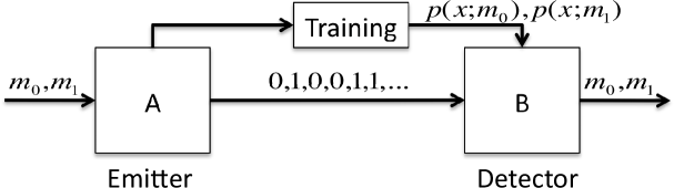
(a) An IR system based on classical probability. A document is like an emitter of binary symbols referrint to term occurrence. The probability that $1$ occurs depends on a parameter that in turn depends on relevance. After training the probability distributions, the system B, which acts as a detector, decides whether a symbol is emitted by a relevant document.

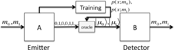
(b) An IR system equipped with an oracle based on vector probability works as the system of Figure 1(a) until symbols reaches an oracle which produces other symbols. The symbols produced by the oracle are vectors. After training the probability distributions, the system B, which acts as a detector, decides whether a vector is emitted by a relevant document.

Figure 1: IR decision as an emitter and detector problem.

We organize the paper as follows. The paper gives an intuitive view of the our contribution in Section 2 and sketches how an IR system built on the premise of Quantum Theory can outperform any other system. Section 3 briefly reviews the classical probability of relevance before introducing the notion of vector probability in Section 4. Section 5 is one of the central sections of the paper because it introduces the optimal vectors which are exploited in Section 6 where we provide our main result, that is, the fact that a system that ranks documents according to the probability of occurrence of the optimal vectors in the documents is always superior to a system which ranks documents according to the classical probability of relevance which is based on sets. Section 7 addresses the case of BM25 and how it can be framed within the theory. An experimental study is illustrated in Section 8 for measuring the degree to which vector probabilistic models outperforms classical probabilistic models if a realistic test collectio is used. The feasibility of the theory is strongly dependent on the existence of an oracle which tells whether optimal vector occur in documents; this issue is discussed in Section 9. After surveying the related work in Section 10, we conclude with Section 11. The appendix includes the definitions used in the paper and the proofs of the theoretical results.

2 Intuitive View

Before entering into mathematics, Figure 1 depicts an intuitive view of what is illustrated in the rest of the paper. Suppose that relevance and non-relevance are two events $m_{0},m_{1}$ occurring with prior probability $1-\xi$ and $\xi$, respectively. Document A is in either relevant or non-relevant. Let’s view A as an emitter of binary symbols $0,1$ referring to presence or absence of a given index term. (We use the binary symbol and relevance for the sake of clarity.) On the other side, an IR system B acts as a detector which has to decide whether a symbol comes out from either a relevant or a non-relevant document. The B’s decision is taken on the basis of some feedback mechanism and on the relevance and non-relevance probability distributions which has been appropriately estimated on received symbols. An IR system that implements classical probability decides about relevance without any transformation of the received symbols (Figure 1(a)) whereas a IR system that implements vector probability decides about relevance after a transformation of the received symbols carried out by an oracle which outputs new symbols which cannot be straightforwardly derived from the received symbols (Figure 1(b)) but can be defined as vectors [4]. In this paper, we show that when B is equipped with such an oracle, then it does significantly outperform any other IR system which implements any classical probabilistic model. We theoretically measure the improvement in effectiveness on the basis of a mathematical proposition which holds for every IR system described in Figure 1.

3 Probability of Relevance

An IR system performing like detector B of Figure 1(a) computes the probabilities that a symbol (e.g., an index term) occurs in relevant documents and in non-relevant documents. According to the intuitive view in terms of emitters and detectors provided in Section 2, the probability that a symbol (e.g., an index term) occurs in relevant documents and in non-relevant documents is called, respectively, probability of detection ($P_{d}$) and probability of false alarm ($P_{0}$). These probabilities are also known as expected recall and fallout, respectively [10]. The system decides whether a document is retrieved by

$$\frac{P_{d}(1-P_{0})}{P_{0}(1-P_{d})} > \lambda$$ (1)

where $\lambda$ is an appropriate threshold, and ranks the retrieved documents by using the left side of (1). For instance, when indipendent Bernoulli random variables are used, we have that

$$P_{d}\propto\Pi_{j=1}^{k}p_{j}^{x_{j}}(1-p_{j})^{1-x_{j}}\qquad P_{0}\propto\Pi_{j=1}^{k}q_{j}^{x_{j}}(1-q_{j})^{1-x_{j}}$$

where $p_{j},q_{j}$ are the probabilities that term $j$ occurs in relevant, non-relevant documents and the $x_{j}$’s belong to the region of acceptance. Depending on the available evidence the probabilities are estimated as accurately as possible and are transformed into weights (e.g., the binary weight or the BM25 illustrated in [12, page 340]).

The Probability Ranking Principle (PRP) defines the optimal document subsets in terms of expected recall and fallout. Thus, the optimal document subsets are those maximizing effectiveness. The PRP states that, if a cut-off is defined for expected fallout, that is, probability of false alarm, we would maximize expected recall if we included in the retrieved set those documents with the highest probability of relevance [10, page 297], that is, probability of detection. When a collection is indexed, each document belongs to subsets labeled by the document index terms and the documents in a subset are indistinguishable. In fact, (1) optimally ranks subsets whose documents are represented in the same way (e.g., the documents which are indexed by a given group of terms or share the same set of feature values). In terms of decision, if fallout is fixed, the PRP permits to decide whether a document (subset) should be retrieved with the minimum probability of error.

4 Vector Probability

When using classical probability term occurrence would correspond to disjoint document subsets (i.e., a subset corresponds to an index term occurring in every document of the subset). When using vector probability, term occurrence corresponds to a document vector subspace which is spanned by the orthonormal vector either $|0\rangle$ or $|1\rangle$ representing, respectively, absence and presence of a given term. (For the sake of clarity, we consider a single term, binary weights and binary relevance as depicted in Figure 1.)

As relevance is an event, two vectors represent binary relevance: a relevance vector $|m_{0}\rangle$ represents non-relevance state and an orthogonal relevance vector $|m_{1}\rangle$ represents relevance state. Relevance vectors and occurrence vectors belong to a common vector space and thus can be defined in terms of a given orthonormal basis of that space.

In a vector space, a random variable is a collection of values and of vectors (or projectors). The vectors are mutually orthonormal and 1:1 correspondence with the values.

Let $x$ be a random variable value (e.g., term occurrence) and $m$ be a conditioning event (e.g., relevance). In Quantum Theory, $|m\rangle$ is also known as state vector and is a specialization of a density operator, that is, a Hermitian and unitary trace operator. The vector probability that ${x}$ is observed given ${m}$ is $\left|\langle x|m\rangle\right|^{2}$. When a density operator $\rho$ and an event is represented by projector $\mathbf{P}$, the vector probability of the event conditioned to the density operator is given by Born’s rule, that is, $\mathrm{tr}(\rho\mathbf{P})$. When $\rho=|m\rangle\langle m|$ and $\mathbf{P}=|x\rangle\langle x|$, vector probability is a specialization of Born’s rule. (See [5].)

It is possible to show that

Proposition 1

A classical probability distribution can be equivalently expressed using vector probability.

The proof is in the appendix.

5 Optimal Vectors

In this section, we reformulate the PRP by replacing subsets with vector subspaces, namely, we replace the notion of optimal document subset with that of optimal vectors (or, vector subspaces). Such a reformulation allows us to compute the optimal vectors that are more effective than the optimal document subsets. To this end, we define a density matrix representing a probability distribution that has no counterpart in, but that is an extension of classical probability. Such a density matrix is the outer product of a relevance vector by itself. When classical probability is assumed, a decision under uncertainty conditions taken upon this density matrix is equivalent to (1) as illustrated in [7]. (See the appendix and [7] as for the details.) When vector probability is assumed, a decision under uncertainty conditions taken upon this density matrix is based upon a different region of acceptance. Hence, we leverage the following Helstrom’s lemma because it is the rule to compute the optimal vectors.

Lemma 1

Let $|m_{1}\rangle,|m_{0}\rangle$ be the relevance vectors. The optimal vectors $|\mu_{0}\rangle,|\mu_{1}\rangle$ at the highest probability of detection at every probability of false alarm is given by the eigenvectors of

$$|m_{1}\rangle\langle m_{1}|-\lambda|m_{0}\rangle\langle m_{0}|$$ (2)

whose eigenvalues are positive.

Proof.

See [4]. ∎

(a) Non-optimal vectors are mutually orthogonal and asymmetrically placed around $|m_{0}\rangle,|m_{1}\rangle$

(b) Optimal vectors are mutually orthogonal and symmetrically placed around $|m_{0}\rangle,|m_{1}\rangle$

Figure 2: Geometry of decision and vectors

The optimal vectors always exist due to the Spectral Decomposition theorem [3]; therefore they are mutually orthogonal because are eigenvectors of (2); moreover, they can be defined in the space spanned by the relevance vectors. The angle between the relevance vectors $|m_{1}\rangle,|m_{0}\rangle$ determines the geometry of the decision of the emitter of Figure 1(b) – geometry means the probability distributions of the events. Therefore, the probability of correct decision and the probability of error are given by the angle between the two relevance vectors and by the angles between the vectors and the relevance vectors. Figure 2(a) depicts the geometry of the optimal vectors. (The figure is in the two-dimensional space for the sake of clarity, but the reader should generalize to higher dimensionality than two.) Suppose $|e_{1}\rangle,|e_{0}\rangle$ are two any other vectors. The angles $\eta_{0},\eta_{1}$ between the vectors and the relevance vectors $|m_{0}\rangle,|m_{1}\rangle$ are related with the angle $\gamma$ between $|m_{0}\rangle,|m_{1}\rangle$ because the vectors are always mutually orthogonal and then the angle is $\frac{\pi}{2}=\eta_{0}+\gamma+\eta_{1}$. The optimal vectors are achieved when the angles between an vector and a relevance vector are equal to

$$\theta=\frac{1}{2}\left(\frac{\pi}{2}-\gamma\right)$$ (3)

The rotation of the non-optimal vectors such that (3) holds, yields the optimal vectors $|\mu_{1}\rangle,|\mu_{0}\rangle$ as Figure 2(b) illustrates: the optimal vectors are “symmetrically” located around the relevance vectors. If any two vectors are rotated in an optimal way, we can achieve the most effective document vector subspaces (or, vectors) in terms of expected recall and fallout. These vectors cannot be ascribed to the subsets yielded by dint of the PRP, the latter impossibility being called incompatibility [13, 5].

6 Vector Probability of Relevance

In this section, we leverage Lemma 1 to introduce the optimal vectors in IR. We define $|m_{0}\rangle$ and $|m_{1}\rangle$ as:

$$|m_{0}\rangle=\left(\begin{array}[]{c}\sqrt{p(1;m_{0})}\\ \sqrt{p(0;m_{0})}\end{array}\right)\qquad|m_{1}\rangle=\left(\begin{array}[]{c}\sqrt{p(1;m_{1})}\\ \sqrt{p(0;m_{1})}\end{array}\right)$$ (4)

Note that, according to Born’s rule $|\langle m_{0}|1\rangle|^{2}=p(1;m_{0})$ and $|\langle m_{1}|1\rangle|^{2}=p(1;m_{1})$, thus (4) reproduce the classical probability distributions.

If the oracle of Figure 1(b) exists, an IR system performing like detector B computes the probabilities that the transformation of a binary symbol referring to an index term, into $|\mu_{0}\rangle$ or $|\mu_{1}\rangle$ occurs in relevant documents and in non-relevant documents. The former is called vector probability of detection ($Q_{d}$) and the latter is called vector probability of false alarm ($Q_{0}$). These probabilities are the analogous of $P_{0},P_{d}$. But, if $|\mu_{0}\rangle,|\mu_{1}\rangle$ are the mutually exclusive symbols yielded by the oracle, we have that

$$Q_{0}=|\langle m_{0}|\mu_{1}\rangle|^{2}\qquad Q_{d}=|\langle m_{1}|\mu_{1}\rangle|^{2}$$ (5)

The latter expression is not the same probability distribution as (4) because it refers to different events. According to [4], we have that the vector probability of error and the vector probability of correct decision are defined, respectively, as

$$Q_{e}=\frac{1}{2}\left(1-\sqrt{1-4\xi(1-\xi)|X|^{2}}\right)\qquad Q_{c}=1-Q_{e}$$ (6)

Both probabilities depend on

$$|X|^{2}=\left(\sqrt{p(1;m_{0})p(1;m_{1})}+\sqrt{(1-p(1;m_{0}))(1-p(1;m_{1}))}\right)^{2}$$ (7)

which is a measure of the distance between two probability distributions as proved in [4, 14]. As the probability distributions refer to relevance and non-relevance, $|X|^{2}$ is a measure of the distance between relevance and non-relevance. An example may be useful.

Suppose, for example, that the probability distributions are $p(1;m_{0})=\frac{4}{5}$, $p(1;m_{1})=1$. If relevance and non-relevance are equiprobable, $P_{e}=\frac{1}{2}\left(P_{0}+1-P_{d}\right)=\frac{2}{5}$ and $P_{c}=\frac{1}{2}\left(1-P_{0}+P_{d}\right)=\frac{3}{5}$. When $\lambda=1$, the optimal vectors are the eigenvectors of

$$\left(\begin{array}[]{cc}\frac{1}{5}&-\frac{2}{5}\\ -\frac{2}{5}&-\frac{1}{5}\end{array}\right)$$

that is,

$$\left(|\mu_{0}\rangle,|\mu_{1}\rangle\right)=\left(\begin{array}[]{cc}-\frac{1}{2}+\frac{\sqrt{5}}{2}&1\\ -\frac{1}{2}-\frac{\sqrt{5}}{2}&1\end{array}\right)\qquad$$ (8)

These vectors can be computed in compliance with [1]. Hence, $Q_{e}=\frac{1}{10}\left(5-\sqrt{5}\right)$, which is less than $P_{e}$.

The following theorem that is our main result shows that the latter example is not an exception.

Theorem 1

If $p(x;m_{j}),j=0,1$ are two arbitrary probability distributions conditioned to $m_{0},m_{1}$, the latter indicating the probability distribution of term occurrence in non-relevant documents and in relevant documents, respectively, then

$$Q_{e}\leq P_{e}$$ (9)

Proof.

See Section Proof of Theorem 1. ∎

Hence, if we were able to find the optimal vectors, retrieval performance of the detector B of Figure 2(b) would always be higher than retrieval performance of the detector B of Figure 2(a).

7 Getting Beyond the State-of-the-Art

The development of the theory assumed binary weights for the sake of clarity. In the event of non-binary weights, e.g., BM25, we slightly fit the theory as follows. If we do the development of the BM25 illustrated in [12] in reverse, we can find that the underlying probability distribution is

$$b(t_{j};m_{i}) = B_{i,j}p(1;m_{i})^{t_{j}}(1-p(1;m_{i}))^{-t_{j}}$$ (10)

$$t_{j} =$$ BM25 saturation factor (11)

$$B_{i,j} = \left\{\begin{array}[]{ll}\frac{1}{n}&p(1;m_{i})=\frac{1}{2}\\ \frac{\log\frac{1-p(1;m_{i})}{p(1;m_{i})}}{1-\left(\frac{p(1;m_{i})}{1-p(1;m_{i})}\right)^{n}}&p(1;m_{i})\neq\frac{1}{2}\end{array}\right.$$ (14)

$$n = \max\left\{t_{j}\right\}$$ (15)

thus $b(t_{j};m_{i})$ is the probability that $t_{j}$ for term $j$ is observed under state $m_{i}$. ($B_{i,j}$ is just a normalization factor.) If $b(t_{j};m_{i})$ estimates $p(x_{j};m_{i})$, the theory still works because Theorem 1 is independent of the estimation of $p(x_{j};m_{i})$. Figure 3 depicts an IR system equipped with an oracle based on vector probability estimated with BM25.

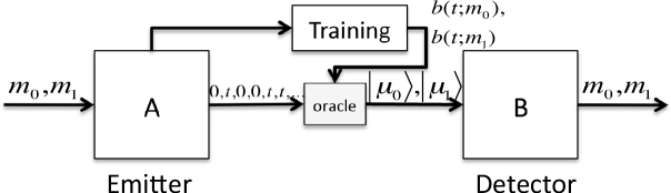
Figure 3: An IR system equipped with an oracle based on vector probability estimated with BM25. A document emits the saturation value if the term occurs, $0$ otherwise. The system B trains the probability distributions using the saturation values. Rather that applying logarithms and computing the BM25 weights, B invokes the oracle that produces the vectors.

8 Experimental Study

In this section we report an experimental study. Our study differs from the common studies conducted in usual IR evaluation because: (1) Theorem 1 already proves that an IR system working as the detector of Figure 2(b) will always be more effective than any other system, therefore, if the former were available, every test would confirm the theorem; (2) as an experimentation that compare two systems using, say, Mean Average Precision requires the implementation of the oracle, which cannot be at present implemented, what we can measure is only the degree to which an IR system working as the detector of Figure 2(b) will outperform any other system.

We have tested the theory illustrated in the previous sections through experiments based on the TIPSTER test collection, disks 4 and 5. The experiments aimed at measuring the difference between $P_{e}$ and $Q_{e}$ by means of a realistic test collection. To this end, we have used the TREC-6, 7, 8 topic sets. The queries are topic titles. We have implemented the following test: $p(x;m)$ has been computed for each topic, query word and $m\in\{m_{0},m_{1}\}$ by means of the usual relative frequency of the word within relevant ($m=m_{1}$) or non-relevant ($m=m_{0}$) documents. In particular, $x=1$ means presence, $x=0$ means absence. Thus, $p(1;m_{0})$ is the estimated probability of occurrence in non-relevant documents and $p(1;m_{1})$ is the estimated probability of occurrence in relevant documents. We have shown in Section 7 that the improvement is independent of probability estimation and then of term weighting.

Consider word crime of Topic No. 301; we have that $p(1;m_{0})=\frac{223}{1234}$ and $p(1;m_{1})=\frac{65}{474}$. Hence, $|X|^{2}=0.998$. (Relevance and non-relevance probability distributions are very close to each other.) Estimation has taken advantage of the availability of the relevance assessments and thus it has been computed on the basis of the explicit assessments made for each topic. Figure 4 depicts $P_{e},Q_{e}$ as function of the prior probability $\xi$. $Q_{e}$ is always greater than $P_{e}$ for every prior probability $\xi$. The vertical distance between the curves is due to the value of $|X|^{2}$, which also yields the shape of the $Q_{e}$ curve, meaning that crime discriminates between relevant and non-relevant documents to an extent depending on $|X|^{2}$ and $\xi$. The average curves computed over all the query words and depicted in Figure 5 give an idea of the overall discriminative power of the topic. In particular, if the total frequencies within relevant and non-relevant documents are computed for each query word and a given topic, average probability of error is computed, for each prior probability. When $\xi$ is close to $\frac{1}{2}$, the curves are indistinguishable because $|X|^{2}$ is very close to $1$. The situation radically changes when Topic No. 344 is considered because $|X|^{2}\approx\frac{9}{25}$; indeed, Figure 6 confirms that $Q_{e}\gg P_{e}$ when $\xi\gg 0$.

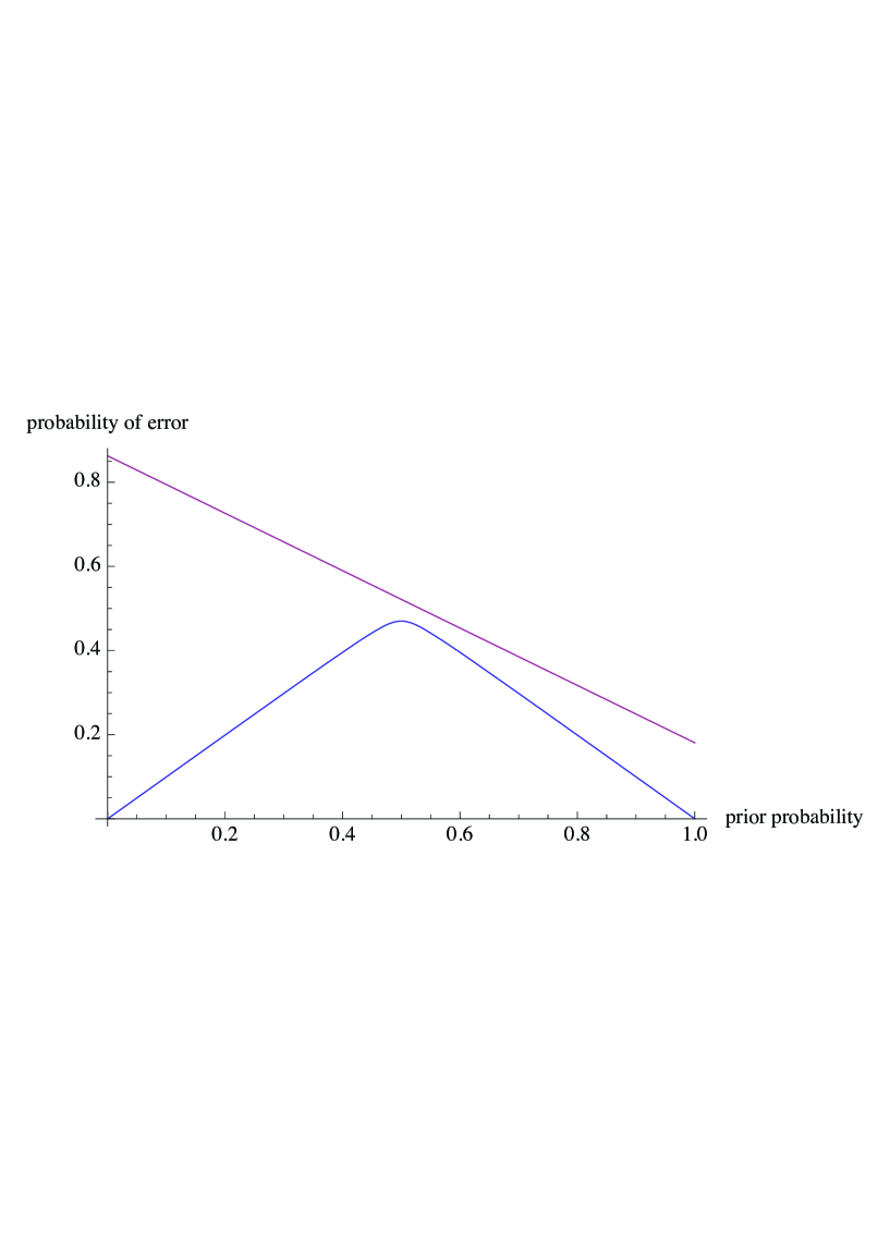
Figure 4: $P_{e}$ and $Q_{e}$ plotted against $\xi$ for word crime of topic $301$.

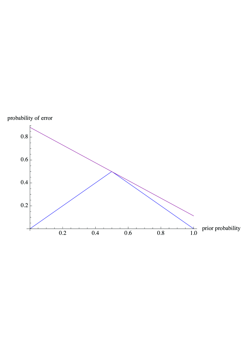
Figure 5: $P_{e}$ and $Q_{e}$ plotted against $\xi$ for topic $301$.

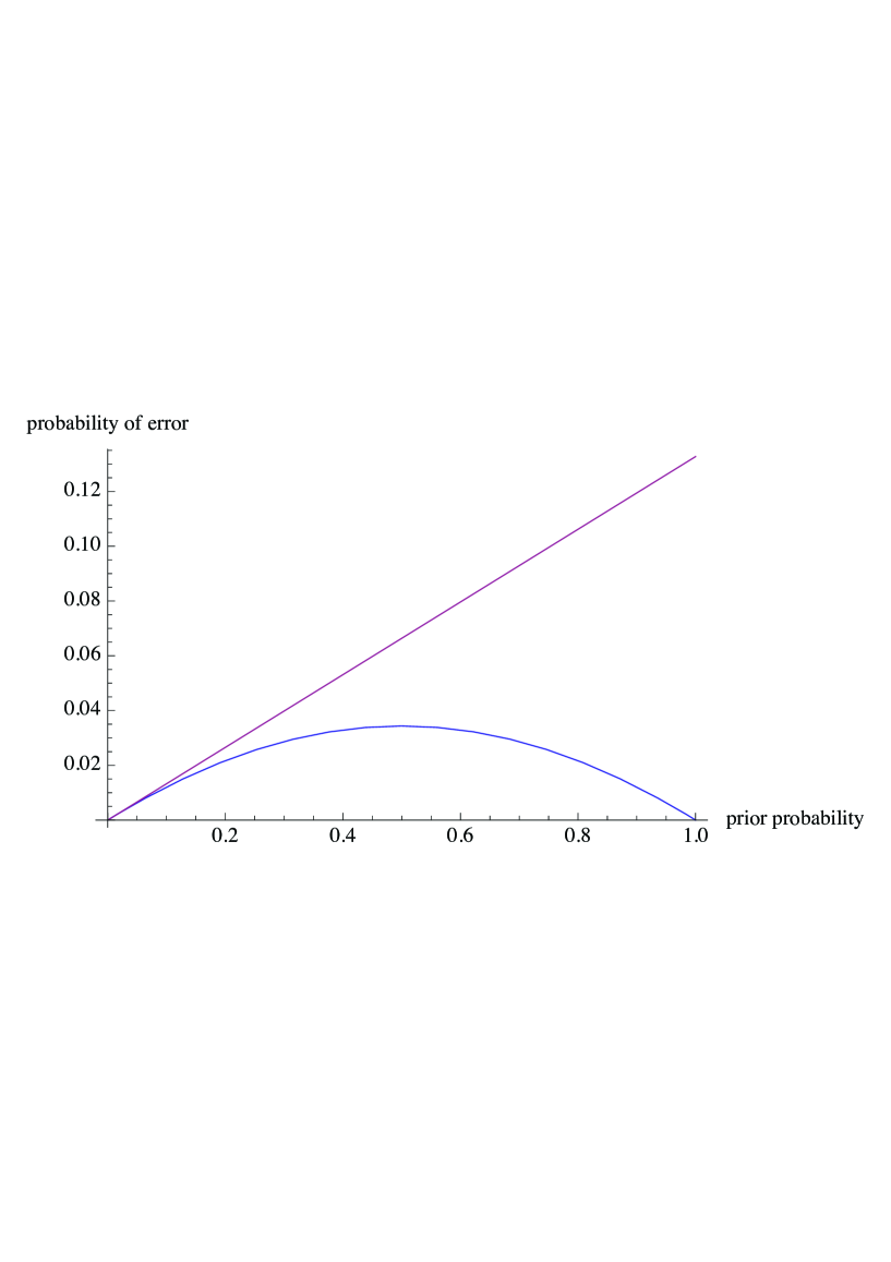
Figure 6: $P_{e}$ and $Q_{e}$ plotted against $\xi$ for topic $344$.

We have also investigated the event that explicit relevance assessment cannot be used because of the lack of reliable judgements for a suitable number of documents. In this event, it is customary to state that $p(1;m_{0})=\frac{n+\frac{1}{2}}{N+1}$ and $p(1;m_{1})=\frac{1}{2}$ [11]. Although pseudo-relevance data is assumed, $|X|^{2}$ and $P_{e}$ can still be computed as function of $p(1;m_{0})$ because the latter are still valid estimations. In particular, we have that

$$|X|^{2}=\frac{1}{2}\left(\sqrt{p(1;m_{0})}+\sqrt{1-p(1;m_{0})}\right)^{2}$$ (16)

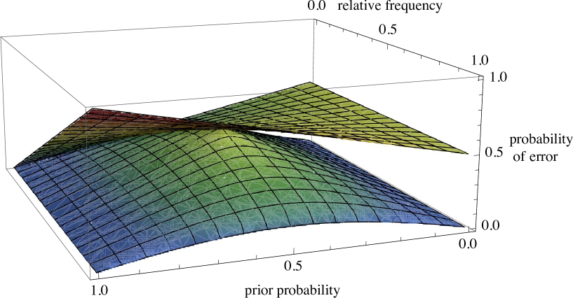
Figure 7: $P_{e}$ and $Q_{e}$ plotted against $\xi$ and relative frequency of a term.

Thus, we can analyze the probabilities of error as functions of $\xi$ and $p(1;m_{0})$. Figure 7 depicts how $P_{e},Q_{e}$ change with $\xi$ and $p(1;m_{0})$; this plot does not depend on a topic, it rather depends on $p(1;m_{0})$, which is a measure of discrimination power of a query word since $\mathrm{IDF}=-\log p(1;m_{0})$. The plot confirms the intuition that $P_{e}$ increases when $p(1;m_{0})$ increases, that is, when IDF decreases. In particular, $P_{e},Q_{e}$ are close to each other when little information about the proportion of relevant documents is available (i.e., $\xi\approx\frac{1}{2}$) and the IDF is not large enough to make a term discriminative. Nevertheless, if some information about the proportion of relevant documents is available (i.e., $\xi$ approaches either $1$ or $0$), $Q_{e}$ becomes much smaller than $P_{e}$ even when the IDF is small (see the bottom-right side of the plot of Figure 7). Table 1 reports the average relative topic word frequency for each topic computed over the query words. The relative frequency gives a measure of query difficulty and can be used to “access” to the plot of Figure 7 to have an idea of $P_{e}$ when using a classical probabilistic IR model and of the improvement that can be achieved through an oracle which can produce the optimal vectors on the basis of the same available evidence as that used to estimate the $p(x;m)$’s.

9 Regarding the Oracle

This section explains why the design of the oracle is difficult. To this end, the section refers to some results of logic in IR reported in some detail in [13]. When binary term occurrence is considered, there are two mutually exclusive events, i.e., either presence ($0$) or absence ($1$). The classical probability used in IR is based on Neyman-Pearson’s lemma which states that the set of term occurrences can be partitioned into two disjoint regions: one region includes all the frequencies such that relevance will be accepted; the other region denotes rejection[8]. If a term is observed from documents and only presence/absence is observed, the possible regions of acceptance are $\emptyset,\{0\},\{1\},\{0,1\}$. When using vectors, the regions of acceptance are $\mathbf{0},|0\rangle\langle 0|,|1\rangle\langle 1|,\mathbf{I}$ which are the projectors to, respectively, the null subspace, the subspace spanned by $|0\rangle$, the subspace spanned by $|1\rangle$, and the entire space.

Consider the symbols $|\mu_{0}\rangle,|m_{1}\rangle$ emitted by the oracle. Vector probability is based on Lemma 1 which states that the set of symbols can be partitioned into two disjoint regions: one region includes all the symbols such that relevance will be accepted; the other region denotes rejection [4]. If a symbol is observed from the oracle, the regions of acceptance are $\mathbf{0},|\mu_{0}\rangle\langle\mu_{0}|,|\mu_{1}\rangle\langle\mu_{1}|,\mathbf{I}$.

Figure 8: The difference between subsets and vector subspaces. The span of $|y\rangle$ and $|x\rangle$ yields the vertical plane, which is spanned by $|e_{1}\rangle$ and $|e_{2}\rangle$ too. If $|e_{2}\rangle$ is intersected by the plane, the result is $|e_{2}\rangle$. But, if $|e_{2}\rangle$ is intersected by $|y\rangle$ and then by $|x\rangle$, the span of the two intersections is $\mathbf{0}$. That is, the distributive law is not admitted by vectors.

The problem is that the subspaces spanned by $|\mu_{0}\rangle,|m_{1}\rangle$ cannot be defined in terms of set operations on the subspaces spanned by $|0\rangle,|1\rangle$. Vector subspaces are equivalent to subsets and they then can be subject to set operations if they are mutually orthogonal [2].

To explain the incompatibility between sets and vectors, we illustrate the fact that the distributive law cannot be admitted in vector spaces as it is in set spaces. Figure 8 shows a three-dimensional vector space spanned by $|e_{1}\rangle,|e_{2}\rangle,|e_{3}\rangle$. The ray (i.e. one-dimensional subspace) $L_{x}$ is spanned by $|x\rangle$, the plane (i.e. two-dimensional subspace) $L_{x,y}$ is spanned by $|x\rangle,|y\rangle$. Note that $L_{e_{1},e_{2}}=L_{x,y}=L_{e_{1},y}$ and so on. According to [5, page 191], consider the vector subspace $L_{e_{2}}\wedge(L_{y}\vee L_{x})$ provided that $\wedge$ means “intersection” and $\vee$ means “span” (and not set union). Since $L_{y}\vee L_{x}=L_{x,y}=L_{e_{1},e_{2}}$, $L_{e_{2}}\wedge(L_{y}\vee L_{x})=L_{e_{2}}\wedge L_{e_{1},e_{2}}=L_{e_{2}}$. However, $(L_{e_{2}}\wedge L_{y})\vee(L_{e_{2}}\wedge L_{x})=0$ because $L_{e_{2}}\wedge L_{y}=0$ and $L_{e_{2}}\wedge L_{x}=0$, therefore

$$L_{e_{2}}\wedge(L_{y}\vee L_{x})\neq(L_{e_{2}}\wedge L_{y})\vee(L_{e_{2}}\wedge L_{x})$$ (17)

thus meaning that the distributive law does not hold, hence, set operations cannot be applied to vector subspaces.

Incompatibility, that is, the invalidity of the distributive law, is due to the obliquity of the vectors. Thus, the optimal vectors cannot be defined in terms of occurrence vectors due to obliquity and a new “logic” must be searched.

The precedent example points out the issue of the measurement of the optimal vectors. Measurement means the actual finding of the presence / absence of the optimal vectors via an instrument or device. The measurement of term occurrence is straightforward because term occurrence is a physical property measured through an instrument or device. (A program that reads texts and writes frequencies is sufficient.) The measurement of the optimal vectors is much more difficult because to our knowledge any physical property does not correspond to an optimal vector.

Despite the difficulty of measuring optimal vectors, one of the main advantages of vector probability and the results reported in this paper is that the effort to design the oracle for any other medium than text is comparable to the effort to design the oracle for text because the limits to observability of the features corresponding to the optimal vectors are actually those undergone when the informative content of images, video and music must be represented. Thus, the question is: what should we observe from a document so that the outcome corresponds to the optimal vector? The question is not futile because the answer(s) would effect automatic indexing and retrieval.

10 Related Work

Van Rijsbergen’s book [13] is the point of departure of our work. It introduced a formalism based on the Hilbert spaces for representing the IR models within a uniform framework. As the Hilbert spaces have been used for formalizing Quantum Theory, the book has also suggested the hypothesis that quantum phenomena have their analogues in IR. In this paper, we are not much interested in investigating whether quantum phenomena have their analogues in IR, in contrast, we use Hilbert vector spaces for describing probabilistic IR models and for defining more powerful retrieval functions.

The latter use of vector spaces in our paper hinges on Helstrom’s book [4], which provides the theoretical foundation for the vector probability and the optimal vectors. In particular, it deals with optical communication and the detectability of optical signals and the improvement of the radio frequency-based methods with which their parameters can be estimated. Within this domain, Helstrom provides the foundations of Quantum Theory for deciding among alternative probability distributions (e.g. relevance versus non-relevance, in this paper). In this paper, we point to a parallel between signal detection and relevance detection by corresponding the need to ferret weak signals out of random background noise to the need to ferret relevance out of term occurrence. Thus, in this paper, Quantum Theory plays the role of enlarging the horizon of the possible probability distributions from the classical mixtures used to define classical distributions to quantum superpositions [7], although decision under conditions of uncertainty can still be treated by the theory of statistical decisions developed by, for example, [8] and used in IR too.

Eldar and Forney’s paper [1] gives an algorithm for computing the optimal vectors and obtains a new characterization of optimal measurement, and prove that it is optimal in a least-squares sense. $|X|^{2}$ is the distance between densities defined in [14] and is implemented as the squared cosine of the angle between the subspaces corresponding to the relevance vectors. The justification of viewing $|X|^{2}$ as a distance comes from the fact that “the angle in a Hilbert space is the only measure between subspaces, up to a constant factor, which is invariant under all unitary transformations, that is, under all possible time evolutions.” [14] The latter is the justification given in [13] of the use of Born’s rule for computing what we call vector probability.

Hughes’ book [5] is an excellent introduction to Quantum Theory. In particular, it addresses incompatibility between observables – we have used that explanation to illustrate the difficulty in implementing the oracle of Figure 1(b). However, in [5], there is no mention of optimal vectors. An introduction to quantum phenomena (i.e., interference, superposition, and entanglement) and Information Retrieval can be found in [7]. In contrast, we do not address quantum phenomena because our aims is to leverage vector space properties in conjunction with probability.

In the IR literature, Quantum Theory is receiving more and more interest. In [9] the authors propose quantum formalism for modeling some IR tasks and information need aspects. In contrast, our paper does not limit the research to the application of an abstract formalism, but exploits the formalism to illustrate how the optimal vectors significantly improve effectiveness. In [15], the authors propose $|X|^{2}$ for modifying probability of relevance; $|X|^{2}$ in conjunction with a cosine of the angle of a complex number are intended to model quantum correlation (also known as interference) between relevance assessments. The implementation of interference is left to the experimenter and that paper provides some suggestions. While [15] shows that vector probability induces a different PRP (called Quantum PRP), this paper shows that vector probability always induces a more powerful ranking than PRP.

11 Conclusions

The research in IR has been traditionally concentrated on extracting and combining evidence as accurately as possible in the belief that the observed features (e.g., term occurrence, word frequency) have to ultimately be scalars or structured objects. The quest for reliable, effective, efficient retrieval algorithms requires to implement the set of features as best one can. The implementation of a set of features is thus an “answer” to an implicit “question”, that is, which is the best set of features for achieving effectiveness as high as possible? However, the research in IR often yields incremental results, thus arising the need to achieve an even better answer. To this end, we suggest to ask another “question”: Which is the best vector subspace?

Definitions and concepts

Definition 1 (Probability Distribution)

A probability distribution maps observable values to the real range $\left[0,1\right]$. As usual, the probabilities are not negative and sums to $1$.

Definition 2 (Classical Probability Distribution)

A classical probability distribution admits only sets of values.

The subsets of values can be defined by means of the set operations (i.e., intersection, union, complement). Thus, one can compute, for instance, the set of relevant documents with a given term frequency.

Definition 3 (Probability of Detection)

It is the probability that a detector decides for relevance when relevance is true; it is called (expected) recall in IR.

Definition 4 (Probability of False Alarm)

It is the probability that a detector decides for relevance when relevance is false; it is called (expected) fallout in IR.

Definition 5 (Region of Acceptance)

It is the set of the observable values that induce the system to decide for relevance. The most powerful region of acceptance yields the maximum probability of detection for a fixed probability of false alarm.

For example, a region of acceptance is a set of term frequencies. The Neyman-Pearson lemma states that the maximum likelihood ratio test defines the most powerful region of acceptance [8].

Definition 6 (Probability of Correct Decision)

$$P_{c}=\xi(1-P_{0})+(1-\xi)P_{d}$$ (18)

provided that $\xi$ the prior probability of non-relevance, $P_{0}$ is the probability of false alarm and $P_{d}$ is the probability of detection.

Definition 7 (Probability of Error)

$$P_{e}=\xi P_{0}+(1-\xi)(1-P_{d})$$ (19)

Of course, $P_{e}+P_{c}=1$. In the following, we adopt the Dirac notation to write vectors so that the reader may refer to the literature on Quantum Theory; a brief illustration of the Dirac notation is in [13].

Definition 8 (Vector Space)

A vector space over a field $\cal F$ is a set of vectors subject to linearity, namely, a set such that, for every vector $|u\rangle$, there are three scalars $a,b,c\in\cal F$ and three vectors $|v\rangle,|x\rangle,|y\rangle$ of the same space such that $|u\rangle=a|v\rangle$ and $|u\rangle=b|x\rangle+c|y\rangle$. If $|u\rangle$ is a vector, $\langle u|$ is its transpose, $\langle v|u\rangle$ is the inner product with $|v\rangle$ and $|v\rangle\langle u|$ is the outer product with $|v\rangle$. A projector $\mathbf{P}$ is a linear operator acting on a vector space such that $\mathbf{P}^{n}=\mathbf{P}$ for every $n>0$. In particular, $|u\rangle\langle u|$ is the projector to the subspace spanned by $|u\rangle$. If $\left|\langle x|x\rangle\right|^{2}=1$, the vector is normal. If $\langle x|y\rangle=0$, the vectors are mutually orthogonal. A subspace is a span of one or more subspaces if its projector is a linear combination of the projectors of the latter; for example, a ray is a span of a vector, a plane is a span of two rays (or vectors), and so on.

Definition 9 (Random Variable)

In classical probability, a random variable is a collection of values and of sets. The sets are mutually disjoint and 1:1 correspondence with the values.

Proof of Proposition 1

Suppose that $p(x;m)$ is the probability that frequency $x$ is observed given a parameter $m$ corresponding to relevance. Note that $m$ may refer to more than one parameter. However, we assume that $m$ is scalar for the sake of clarity. In the event of binary relevance, $m$ is either $m_{0}$ (non-relevance) or $m_{1}$ (relevance). The expressions

$$|m_{0}\rangle=\sum_{x=0}^{N}a(x;m_{0})|x\rangle$$

$$|m_{1}\rangle=\sum_{x=0}^{N}a(x;m_{1})|x\rangle$$

$$a(x;m)=\pm\sqrt{p(x;m)}$$ (20)

establish the relationship between classical probability distributions and vector probability, namely, between the parameters $m_{0},m_{1}$, the relevance vectors $|m_{0}\rangle,|m_{1}\rangle$ and the observable $X$. The sign of $a(x;m)$ is chosen so that the orthogonality between the relevance vectors is retained. Moreover, the orthogonality of the relevance vectors and the following expression

$$\left|\langle y|m\rangle\right|^{2} = \left|\sum_{x=0}^{N}a(x;m)\langle y|x\rangle\right|^{2}$$ (21)

$$= \left|a(y;m)\right|^{2}\qquad\mbox{due to orthogonality}$$ (22)

$$= p(y;m)$$ (23)

establish the relationship between classical and vector probability of relevance.

Proof of Theorem 1

Consider Figures 2(a) and 2(b). A probability of detection $p_{d}$ and a probability of false alarm $p_{0}$ defines the coordinates of $|m_{0}\rangle$ and $|m_{1}\rangle$ with a given orthonormal basis $|e_{0}\rangle,|e_{1}\rangle$ (that is, an observable):

$$|m_{0}\rangle=\sqrt{1-p_{d}}|e_{0}\rangle+\sqrt{p_{d}}|e_{1}\rangle$$ (24)

$$|m_{1}\rangle=\sqrt{p_{0}}|e_{0}\rangle+\sqrt{1-p_{0}}|e_{1}\rangle$$ (25)

The coordinates are expressed in terms of angles:

$$1-p_{d}=\sin^{2}\eta_{1}\qquad p_{0}=\sin^{2}\eta_{0}$$ (26)

provided that $\eta_{i}$ is the angle between $|m_{i}\rangle$ and $|e_{1}\rangle$.

The probability of error is

$$p_{e}=\xi p_{0}+(1-\xi)(1-p_{d})=\xi\sin^{2}\eta_{0}+(1-\xi)\sin^{2}\eta_{1}$$ (27)

The probability of error is minimum when $\eta_{0}=\eta_{1}=\theta$ as shown in [4, page 99].

But, $\theta$ is exactly the angle between $|m_{i}\rangle,i=0,1$ and $|\mu_{i}\rangle$ and is defined as a result of Equation (3). The probability of error is then minimized when the observable vectors are the $|\mu_{i}\rangle,i=0,1$.

Therefore, $Q_{e}\leq P_{e}$ for all $P_{e}$, that is, for all the observable vectors. As $Q_{c}=1-Q_{e}$, the probability of correct decision is also maximum.

Topic	Av. Relative Frequency	Topic	Av. Relative Frequency	Topic	Av. Relative Frequency
301	0.0458	351	0.0054	401	0.0666
302	0.0063	352	0.0284	402	0.0001
303	0.0008	353	0.0018	403	0.0000
304	0.0026	354	0.0016	404	0.0458
305	0.0054	355	0.0017	405	0.0025
306	0.0088	356	0.0107	406	0.0025
307	0.0074	357	0.0055	407	0.0012
308	0.0001	358	0.0033	408	0.0005
309	0.0052	359	0.0131	409	0.0092
310	0.0104	360	0.0164	410	0.0260
311	0.0128	361	0.0016	411	0.0001
312	0.0000	362	0.0085	412	0.0343
313	0.0003	363	0.0055	413	0.0251
314	0.0026	364	0.0001	414	0.0123
315	0.0029	365	0.0053	415	0.0070
316	0.0000	366	0.0108	416	0.0130
317	0.0001	367	0.0002	417	0.0001
318	0.0379	368	0.0001	418	0.0148
319	0.0124	369	0.0000	419	0.0009
320	0.0045	370	0.0266	420	0.0012
321	0.0112	371	0.0272	421	0.0189
322	0.0510	372	0.0218	422	0.0072
323	0.0005	373	0.0162	423	0.0008
324	0.0421	374	0.0021	424	0.0000
325	0.0002	375	0.0082	425	0.0193
326	0.0007	376	0.0571	426	0.0225
327	0.0020	377	0.0010	427	0.0035
328	0.0007	378	0.0103	428	0.0203
329	0.0217	379	0.0000	429	0.0023
330	0.0236	380	0.0103	430	0.0034
331	0.0808	381	0.0026	431	0.0094
332	0.0495	382	0.0059	432	0.0278
333	0.0026	383	0.0067	433	0.0039
334	0.0077	384	0.0119	434	0.0188
335	0.0042	385	0.0110	435	0.0226
336	0.0126	386	0.0134	436	0.0023
337	0.0003	387	0.0060	437	0.0150
338	0.0040	388	0.0015	438	0.0203
339	0.0161	389	0.0144	439	0.0024
340	0.0143	390	0.0054	440	0.0087
341	0.0343	391	0.0340	441	0.0024
342	0.0031	392	0.0000	442	0.0014
343	0.0282	393	0.0021	443	0.0345
344	0.0023	394	0.0599	444	0.0001
345	0.0336	395	0.0014	445	0.0111
346	0.0068	396	0.0157	446	0.0054
347	0.0012	397	0.0008	447	0.0026
348	0.0000	398	0.0199	448	0.0146
349	0.0000	399	0.0012	449	0.0001
350	0.0229	400	0.0035	450	0.0256

Table 1: Average relative frequency per topic.

References

- [1] Y. Eldar and G. Forney. On quantum detection and the square-root measurement. IEEE Transactions on Information Theory, 47(3):858–872, 2001.
- [2] R. B. Griffiths. Consistent quantum theory. Cambridge University Press, 2002.
- [3] P. Halmos. Finite-dimensional vector spaces. Undergraduate Texts in Mathematics. Springer, 1987.
- [4] C. Helstrom. Quantum detection and estimation theory. Academic Press, 1976.
- [5] R. Hughes. The structure and interpretation of quantum mechanics. Harvard University Press, 1989.
- [6] A. Kolmogorov. Foundations of the theory of probability. Chelsea Publishing Company, New York, second edition, 1956.
- [7] M. Melucci and C. van Rijsbergen. Quantum mechanics and information retrieval. In Advanced Topics in Information Retrieval. Springer, Forthcoming.
- [8] J. Neyman and E. Pearson. On the problem of the most efficient tests of statistical hypotheses. Philosophical Transactions of the Royal Society, Series A, 231:289–337, 1933.
- [9] B. Piwowarski, I. Frommholz, M. Lalmas, and K. van Rijsbergen. What can quantum theory bring to information retrieval. In Proceedings of the 19th ACM international conference on Information and knowledge management, CIKM ’10, pages 59–68, New York, NY, USA, 2010. ACM.
- [10] S. Robertson. The probability ranking principle in information retrieval. Journal of Documentation, 33(4):294–304, 1977.
- [11] S. Robertson and K. Sparck Jones. Relevance weighting of search terms. Journal of the American Society for Information Science, 27:129–146, May 1976.
- [12] S. Robertson and H. Zaragoza. The probabilistic relevance framework: BM25 and beyond. Foundations and Trends in Information Retrieval, 3(4):333–389, 2009.
- [13] K. van Rijsbergen. The geometry of information retrieval. Cambridge University Press, UK, 2004.
- [14] W. K. Wootters. Statistical distance and Hilbert space. Phys. Rev. D, 23(2):357–362, Jan 1981.
- [15] G. Zuccon and L. Azzopardi. Using the quantum probability ranking principle to rank interdependent documents. In Proceedings of the European Conference on Information Retrieval Research (ECIR), pages 357–369, 2010.