A note on fractional linear pure birth and pure death processes in epidemic models

Abstract

In this note we highlight the role of fractional linear birth and linear death processes recently studied in Orsingher et al. [9] and Orsingher and Polito [8], in relation to epidemic models with empirical power law distribution of the events. Taking inspiration from a formal analogy between the equation of self consistency of the epidemic type aftershock sequences (ETAS) model, and the fractional differential equation describing the mean value of fractional linear growth processes, we show some interesting applications of fractional modelling to study ab initio epidemic processes without the assumption of any empirical distribution. We also show that, in the frame of fractional modelling, subcritical regimes can be linked to linear fractional death processes and supercritical regimes to linear fractional birth processes.

Moreover we discuss a simple toy model to underline the possible application of these stochastic growth models to more general epidemic phenomena such as tumoral growth.

Keywords: ETAS model, fractional branching, birth process, death process, Mittag–Leffler functions, Wiener–Hopf integral.

1 Introduction

In recent years there has been a growing interest in fractional calculus modelling in different fields of applied sciences, from rheology to biology (see for example Podlubny [10], Debnath [2], Mainardi [6], Diethelm [3]). It is well known that fractional derivatives are a good instrument to handle memory mechanisms, which are very useful in studying anomalous diffusion processes. Indeed, the fractional derivative in the sense of Caputo is defined by a convolution of a power law with the ordinary derivative of the function, thus underlining its importance as an instrument to describe processes with emerging power law distributions. Recent papers [9, 8] describe fractional processes of death and birth in which the integer-order derivative in the difference-differential equations governing the state probabilities of the related classical models, is replaced with the Caputo fractional derivative. In this note we apply this generalisation to the study of epidemic processes. In particular, we take inspiration from an interesting analogy between the self consistency equation of the ETAS (epidemic type aftershock sequences) model, used with success in statistical seismology, and the equation governing the mean behaviour of the fractional linear death model. The ETAS model, based on epidemic branching processes, [11], is used to describe seismic sequences of shocks in the context of a stochastic model in which each aftershock may trigger other aftershocks. This model is based on empirical power law distributions emerging from the analysis of seismic catalogues, i.e., the modified Omori law on the time distribution of aftershocks and the Gutenberg–Richter law for the distribution of their magnitudes. These types of models are greatly studied in literature (see for example Sornette and Sornette [12], Helmstetter and Sornette [4]) and used in assessing seismic risk [5]. The self consistency equation of the ETAS model [12] is the classical Wiener–Hopf integral equation, but with simple handling it can be considered to be a fractional integral equation similar to the equation governing the mean behaviour of the fractional linear death model. Using this analogy we suggest an interpretation of the fractional death and birth processes in the framework of epidemic models with power law distributions (e.g. ETAS). The organization of this paper is the following: in Section 2 we recall the fundamental results on fractional death and fractional birth models; in Section 3 we describe the analytic formulation of the ETAS model from which we took inspiration for the discussion which follows in Section 4, that is the relations between the ETAS and fractional processes; in Section 5, in order to highlight the utility of this stochastic framework, we give an example of application of this formalism to describe tumoral growth; finally, in Section 6 we discuss the main results obtained.

2 Fractional linear pure death and pure birth processes

Recently, in Orsingher et al. [9], section 2, the fractional linear death process was introduced and studied. The fractional linear death process is a generalisation of the well-known classical linear death process. Fractionality is obtained by replacing the integer-order derivative in the difference-differential equations governing the state probabilities of the classical model with the Caputo fractional derivative (3.7) of order $\nu\in(0,1)$. We exclude the case $\nu=1$ as it is trivial and coincides with the classical case. Let $n_{0}$ be the size of the population at time $0$ and let $M^{\nu}(t)$, $t>0$, $\nu\in(0,1)$, be the number of components in the population in the fractional linear death process at time $t$.

The state probabilities $\text{Pr}\{M^{\nu}(t)=k|M^{\nu}(0)=n_{0}\}$, $0\leq k\leq n_{0}$, solve the following Cauchy problem:

$$\begin{cases}D^{\nu}p_{k}(t)=\mu(k+1)p_{k+1}(t)-\mu kp_{k}(t),&0\leq k\leq n_{0},\>\nu\in(0,1),\\ p_{k}^{\nu}(0)=\begin{cases}1&\text{if $k=n_{0}$},\\ 0&\text{if $k<n_{0}$},\end{cases}\end{cases}$$ (2.1)

where $\mu>0$ is the death intensity and in which we consider that $p_{n_{0}+1}(t)=0$.

We recall the following fundamental theorem [9, page 73]:

Theorem 2.1.

The distribution of the fractional linear death process $M^{\nu}(t)$, $t>0$ with $n_{0}$ initial individuals and death rates $\mu_{k}=\mu k$, is given by:

$$p^{\nu}_{k}(t) =\text{Pr}\{M^{\nu}(t)=k|M^{\nu}(0)=n_{0}\}$$ (2.2)

$$=\binom{n_{0}}{k}\sum_{r=0}^{n_{0}-k}\binom{n_{0}-k}{r}(-1)^{r}E_{\nu,1}(-(k+r)\mu t^{\nu})$$

where $0\leq k\leq n_{0}$, $t>0$, $\nu\in(0,1)$. The function $E_{\nu,1}(x)$ is the Mittag–Leffler function defined as

$$E_{\nu,1}(x)=\sum_{k=0}^{+\infty}\frac{x^{k}}{\Gamma(\nu k+1)}\qquad x\in\mathbb{R},\>\nu>0$$

In the same paper it is also shown that the mean value $\mathbb{E}M^{\nu}(t)$, $t>0$, of the fractional linear pure death process satisfies the fractional differential equation

$$\begin{cases}D^{\nu}\mathbb{E}M^{\nu}(t)=-\mu\mathbb{E}M^{\nu}(t),&t>0,\>\nu\in(0,1),\\ \mathbb{E}M^{\nu}(0)=n_{0},\end{cases}$$ (2.3)

which can be easily solved by means of the Laplace transform, obtaining

$$\mathbb{E}M^{\nu}(t)=n_{0}E_{\nu,1}(-\mu t^{\nu}),\qquad t>0,\>\nu\in(0,1).$$ (2.4)

In Orsingher and Polito [8], the fractional pure birth process $\mathfrak{N}^{\nu}(t)$, $t>0$, $\nu\in(0,1)$, was studied with similar methods to those used for the fractional death. For the sake of our discussion, we recall only the fractional differential equation which governs the mean value $\mathbb{E}\mathfrak{N}^{\nu}(t)$, $t>0$, referring to the original paper for further details:

$$\begin{cases}D^{\nu}\mathbb{E}\mathfrak{N}^{\nu}(t)=\gamma\mathbb{E}\mathfrak{N}^{\nu}(t),&t>0,\>\gamma>0,\nu\in(0,1),\\ \mathbb{E}\mathfrak{N}^{\nu}(0)=1,\end{cases}$$ (2.5)

where $\gamma$ is the birth intensity. The solution to (2.5) reads:

$$\mathbb{E}\mathfrak{N}^{\nu}(t)=E_{\nu,1}(\gamma t^{\nu}),\qquad t>0.$$ (2.6)

Recalling the definition of Mittag–Leffler function, we remark that asymptotically, it has a power law decay (see for example Ogata [7]).

Finally, a subordination relation is verified for the fractional linear death and fractional linear birth processes. For example, for the fractional death, we have that

$$M^{\nu}(t)\overset{\text{d}}{=}M(V_{t}^{\nu}),\qquad t>0,\>\nu\in(0,1),$$ (2.7)

where the equality is intended for the one-dimensional distribution and $V_{t}^{\nu}$, $t>0$, $\nu\in(0,1)$, is the right-inverse process of the $\nu$-stable subordinator $S^{\nu}_{x}$, $x>0$, $\nu\in(0,1)$, i.e.

$$V_{t}^{\nu}=\inf\{x>0\colon S^{\nu}_{x}>t\}.$$ (2.8)

3 Analytical formulation of the ETAS model

In this section we follow Sornette and Sornette [12] to define the master self consistency equation of the ETAS model. We do not discuss in detail the modellistic aspects of the ETAS model (see for example Helmstetter and Sornette [4]). Briefly, it can be considered as a simple branching model in which each afteshock may trigger other succeding aftershocks in a cascade process. It is therefore natural to regard this as an epidemic process in which a given parent event of a certain magnitude, occurring at time $t=0$, gives birth to other child events with rate:

$$\phi(t)\mathrm{d}t=(1-k)\theta t_{0}^{\theta}\frac{1}{t^{1+\theta}}H(t-t_{0}),\qquad t>0,$$ (3.1)

where $H(x)$, $x\in\mathbb{R}$, is the Heaviside step function, and $(1-k)t_{0}^{\theta}/t^{1+\theta}$ is the modified local Omori law on the time occurrence of the aftershocks. In the following, we focus our attention only on time behaviour and decay of this cascade process. The self consistency equation, describing the rate of seismicity at a given time $t$, reads [12]:

$$N(t)=(1-k)\int_{0}^{t-t_{0}}N(\tau)\theta t_{0}^{\theta}(t-\tau)^{-(1+\theta)}\,\mathrm{d}\tau,$$ (3.2)

where $\int_{0}^{+\infty}\phi(t)\mathrm{d}t=(1-k)$, is the branching ratio, i.e., the average number of aftershocks generated by each event; $t_{0}$ is a time delay with respect to the mainshock that occurs at time zero. Note that equation (3.2) is the classical Wiener–Hopf integral equation with a power law kernel. In Sornette and Sornette [12], and Helmstetter and Sornette [4], an interesting discussion of the analytic solution to this equation was given and, in particular, three different regimes for the seismic rate $N(t)$, were found:

• $k>0$ and $\theta>0$: subcritical regime, less than one child per parent;

• $k<0$ and $\theta>0$: supercritical regime. A transition from an Omori decay with exponent $p=1-\theta$ to an explosive increase of the seismicity rate;

• $\theta<0$ and $k>0$: a transition from an Omori law with exponent $1-|\theta|$ to an exponentially increasing seismicity rate for large values of time.

In Sornette and Sornette [12], a first discussion about the analytic solution of the self consistency equation was given. The authors found a characteristic time $t^{*}$, function of all the ETAS parameters, acting as a cut-off between the small and the large time behaviour. They discussed this important feature both for the subcritical and supercitical regimes. For the subcritical regime, this means the transition from an Omori exponent $p=1-\theta$ for $t<t^{*}$ to $p=1+\theta$ for $t>t^{*}$, i.e. it implies that the seismic rate decays slowly for small values of $t$. For the supercritical regime the authors found a transition from an Omori power law decay with exponent $p=1-\theta$ for $t<t^{*}$ to an explosive exponential increase. In a successive paper, Helmstetter and Sornette [4] generalised their analysis, by taking into consideration also the Gutenberg–Richter distribution. What is more interesting for the sake of our discussion, is that they also analysed the third regime, i.e. $\theta<0$. This case needs more attention, because the integral $\int_{0}^{\infty}\phi(t)\mathrm{d}t\sim\int_{0}^{\infty}1/(t+1)^{1+\theta}\mathrm{d}t$ becomes unbounded, thus implying an infinite branching ratio. The authors explained this, apparently meaningless result saying that the number of children created beyond any time $t$ exceeds the numbers of children created until time $t$. This interpretation is also confirmed by the discussion on the analytic solution related to this third regime, in which another charateristic time $\tau$ of transition from an anomalous slow decay for $t<\tau$ and an explosive exponential increase for $t>\tau$, similar to the supercritical case, was found. Therefore, this case, and the supercritical case, have a modellistic utility proven to be useful to understand phenomena with anomalous slow seismic decay for small values of time, although they appear meaningless for large values of time. We refer to Helmstetter and Sornette [4] for a thorough discussion on the meaning of the regimes of the ETAS model.

Before going ahead, we give some mathematical remarks on equation (3.1). For example, in the last case ($\theta<0$), we can rewrite it in the following manner:

$$N(t)=-(1-k)|\theta|\int_{0}^{t}N(\tau)t_{0}^{\theta}(t-\tau)^{-(1-|\theta|)}\,\mathrm{d}\tau,\qquad t>0,$$ (3.3)

where we have done the approximation $t-t_{0}\sim t$, the time delay being small with respect to the total time interval. By recalling the definition of Riemann–Liouville fractional integral of order $\alpha>0$ [10]

$$J^{\alpha}f(t)=\frac{1}{\Gamma(\alpha)}\int_{0}^{t}f(\tau)(t-\tau)^{-(1-\alpha)}\,\mathrm{d}\tau,\qquad\alpha>0,\>t>0,$$ (3.4)

with $\Gamma(\alpha)$ the Euler Gamma function, it is easy to rewrite the equation (3.3) as a fractional integral equation. Indeed we have that

$$N(t)=-\lambda J^{|\theta|}N(t),\qquad t>0,\>\theta<0,$$ (3.5)

where $\lambda=(1-k)|\theta|\Gamma(|\theta|)$. Finally, we arrive at the following fractional differential equation:

$$D^{|\theta|}N(t)=-\lambda N(t),\qquad t>0,\>\theta<0,$$ (3.6)

where $D^{|\theta|}$ is the Caputo fractional derivative of order $|\theta|>0$, defined as [10]

$$D^{|\theta|}N(t)=\frac{1}{\Gamma(m-|\theta|)}\int_{0}^{t}\frac{\frac{\mathrm{d}^{m}}{\mathrm{d}\tau^{m}}N(\tau)}{(t-\tau)^{|\theta|-m+1}}\mathrm{d}\tau,$$ (3.7)

where $m=\lceil|\theta|\rceil$.

Equation (3.5) can thus be written as a simple linear fractional differential equation. Equation (3.6), in the case $\theta\in(-1,0)$, with the initial condition $N(0)=n_{0}$, $n_{0}\in\mathbb{N}$ (meaning that the initial rate of seismicity is $n_{0}$), can be easily solved as we have shown in the previous section.

Finally, we realize that the ETAS self consistency equation is formally similar to equation (2.3) governing the mean behaviour of the fractional linear death process. Furthermore, the supercritical regime with explosive growth can be linked in the same way to the fractional linear pure birth process. In the next section, we discuss similarities and differences between these models.

4 Relations between self consistency equation of the ETAS model and fractional birth or death processes

Taking inspiration from the formal analogy shown in Section 3, here, we discuss the analytical behaviour of the rate $N(t)$, $t>0$, in the framework of fractional death and fractional birth processes, considering, on the one hand, the behaviour predicted by them, and, on the other hand, the physical meaning of these predictions in the framework of the ETAS model. In short, the rate of seismicity $N(t)$, $t>0$, is considered here as the mean behaviour of an underlying fractional linear death or birth process.

Similarly to the ETAS model, starting from equation (3.6) describing the rate of an epidemic process, we can distinguish two regimes:

• if $\lambda>0$, we have

  $$D^{\nu}N(t)=-\lambda N(t),\qquad t>0,\;\nu\in(0,1).$$ (4.1)

  As we have shown, it is identical to the fractional differential equation arising in the fractional death process. Physically it corresponds to the subcritical regime in the framework of the ETAS model. However we must underline some differences, remembering that our formal analogy is not rigorously an identity. We observe a strong exponential decay for small values of $t$ and an asymptotic power law decay when $t\rightarrow\infty$. Thus, we have a reasonable physical picture for cases with a slow decay for large times, but this prediction is slightly different from that of ETAS.

  In Fig. 1 the solution to the Cauchy problem composed by (4.1) and the initial condition $N(0)=n_{0}=1$, for some values of $\nu$, is shown; it corresponds to the mean value of the linear fractional death process. Note the fast decay for small values of $t$.

  

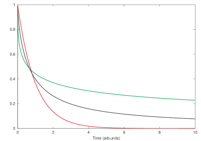
  Figure 1: The mean value of the linear fractional death process with $\nu=1$ (red), $\nu=0.7$ (black) and $\nu=0.4$ (green).

• if $\lambda<0$ we have the following equation:

  $$D^{\nu}N(t)=|\lambda|N(t),\;\nu\in(0,1).$$ (4.2)

  This corresponds to the fractional differential equation arising in the linear fractional birth process. This case is equivalent to the supercritical regime of the ETAS model. Indeed, we have an explosive growth. Fig. 2 presents the solution to the Cauchy problem composed by (4.2) and the initial condition $N(0)=1$. We have an exponential growth, as for the supercritical regime of the ETAS model.

  

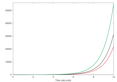
  Figure 2: The mean value of the linear fractional birth process with $\nu=1$ (red), $\nu=0.7$ (black) and $\nu=0.4$ (green).

5 An application of the fractional pure birth process: theoretical model of tumoral growth

Beyond the formal analogy with the ETAS model we can explain the utility of our proposal with a simple toy model about tumoral growth. In the following we show that the fractional linear pure birth process can give an interesting framework to modelling this kind of phenomena and have good agreement with some results in this field. Assume that we have an initial number of infected cells $\mathfrak{N}^{\nu}(0)=n_{0}$. We are interested in building a theoretical model about the growth of cancer cells with respect to time in the dynamics of metastasis. Suppose that this process is described by a linear fractional pure birth model. Therefore we have (see Orsingher and Polito [8]) that the distribution of the population size of cancer cells at time $t$ is given by:

$$\text{Pr}\{\mathfrak{N}^{\nu}(t)=k+n_{0}|\mathfrak{N}^{\nu}(0)=n_{0}\}$$ (5.1)

$$=\binom{n_{0}+k-1}{k}\sum_{r=0}^{k}\binom{k}{r}(-1)^{r}E_{\nu,1}(-(n_{0}+r)\gamma t^{\nu}),\quad t>0,\>\nu\in(0,1],\>\gamma>0.$$

Now, from (5.1), we can infer the probability of a new offspring at the beginning of the process:

$$\text{Pr}\{\mathfrak{N}^{\nu}(\mathrm{d}t)=1+n_{0}|\mathfrak{N}^{\nu}(0)=n_{0}\}$$ (5.2)

$$=n_{0}\left[E_{\nu,1}(-n_{0}\gamma(\mathrm{d}t)^{\nu})-E_{\nu,1}(-\gamma(n_{0}+1)(\mathrm{d}t)^{\nu})\right]\sim n_{0}\frac{\gamma(\mathrm{d}t)^{\nu}}{\Gamma(\nu+1)},$$

by writing only the lower order terms. This result shows that the probability of a new offspring is proportional to the time interval $(\mathrm{d}t)^{\nu}$ and to the initial number of progenitors. This is an interesting picture that can be realistic for a large number of complex growth dynamics with emerging power law behaviour. From the previous analysis, we also have that the average expansion of the population of cancer cells is given by:

$$\mathbb{E}\mathfrak{N}^{\nu}(t)=n_{0}E_{\nu,1}(\gamma t^{\nu}),\qquad t>0.$$ (5.3)

In conclusion we have a theoretical framework that can be used to describe growth processes exhibiting power law expansions.

We discussed this model by referring to the cancer growth dynamics because several works (see for example Dattoli et al. [1], West et al. [13]) studied a similar dynamic starting from the Kleiber law. It is not the purpose of this paper going inside this vaste field of study, but we remark that we have a conceptual well posed model without empirical assumptions. Thus we obtain a probabilistic point of view that is more fundamental with respect to the dynamic of these processes. Finally, we must observe that, in order to make the model more realistic, it is possible to directly generalise the fractional birth process by introducing a saturation threshold. This will be matter of a future paper.

We also notice that the role played by the allometric coefficients in the Kleiber law, in our model, is played by the real order of derivation $\nu$. These allometric coefficients are empirically established; we have the same picture but with only one free fitting parameter. Beyond the probabilistic clear view of the processes, this is also a strong point of this theory,

6 Discussion

We now move to understand the differencess between the ETAS model and the fractional epidemic processes predictions. First, we must identify the real order of derivation $\nu$ with the parameter $\theta$ of the Omori law and $\lambda$ with $\lambda=(1-k)|\theta|\Gamma(|\theta|)$ of the ETAS model. Although we do not have exactly the same cut-off between different regimes as in the ETAS model, we obtain some reasonable agreement for various ranges of the parameters. Moreover, in Helmstetter and Sornette [4], by discussing the self-consistency equation for the supercritical regime, a cut-off between slow decay for small times and explosive growth was found. In our case, the supercritical regime is less meaningful, presenting immediately an exponential growth. On the other hand, from the self-consistency equation (3.2) and by considering the physical behaviour in the subcritical regime, the agreement of the two models is clear, both describing epidemic processes.

At this point, by keeping in mind the relations between the ETAS model and the fractional linear birth or death processes, we make some remarks. We have a generalised analytic model with clear relations with epidemic models. We also notice that in many epidemic processes in complex systems (as in seismology and biology), empirical power law behaviour emerges. We have seen that the prediction on the rate of fractional processes, i.e., the Mittag–Leffler function (generalised exponential), takes into account this behaviour asymptotically. We conclude that the fractional processes we treated in this paper, are an important instrument in order to study epidemic processes which exhibit a rapid decay for small times and slow asymptotic power law decay for large times.

References

- Dattoli et al. [2009] G. Dattoli, C. Guiot, P. Delsanto, P. Ottaviani, S. Pagnutti, and T. Deisboeck. Cancer metabolism and the dynamics of metastasis. Journal of Theoretical Biology, 256:305–310, 2009.
- Debnath [2003] L. Debnath. Recent applications of fractional calculus to science and engineering. Int. J. Math. Math. Sci., 2003(54):3413–3442, 2003.
- Diethelm [2010] K. Diethelm. The Analysis of Fractional Differential Equations. Springer, New York, USA, 2010.
- Helmstetter and Sornette [2002] A. Helmstetter and D. Sornette. Subcritical and supercritical regimes in epidemic models of earthquake aftershocks. J. Geophys. Res., 107:2237–2257, 2002.
- Helmstetter and Sornette [2003] A. Helmstetter and D. Sornette. Predictability in the Epidemic-Type Aftershock Sequence model of interacting triggered seismicity. j. Geophys. Res., 108:2482–2499, 2003.
- Mainardi [2010] F. Mainardi. Fractional Calculus and Waves in Linear Viscoelasticity: An Introduction to Mathematical Models. Imperial College Press, London, UK, 2010.
- Ogata [1998] Y. Ogata. Space-time point process models for earthquake occurences. Ann. Inst. Statist. Math, 50(2):379–402, 1998.
- Orsingher and Polito [2010] E. Orsingher and F. Polito. Fractional Pure Birth Processes. Bernoulli, 16(3):858–881, 2010.
- Orsingher et al. [2010] E. Orsingher, F. Polito, and L. Sakhno. Fractional Non-Linear, Linear and Sublinear Death Processes. J. Stat. Phys., 141(1):68–93, 2010.
- Podlubny [1999] I. Podlubny. Fractional Differential Equations. Academic Press, New York, USA, 1999.
- Saichev and Sornette [2005] A. Saichev and D. Sornette. Vere-Jones’ Self Similar Branching Model. Phys. Rev. E, 72(056122), 2005.
- Sornette and Sornette [1999] A. Sornette and D. Sornette. Renormalization of earthquake aftershocks. Geophys. Res. Lett., 26(13):1981–1984, 1999.
- West et al. [2004] G. West, G. Brown, and B. Enquist. Growth models based on first principles or phenomenology? Functional Ecology, 18:188–196, 2004.