Instantons causing iterative decoding to cycle

Abstract

It is speculated that the most probable channel noise realizations (instantons) that cause the iterative decoding of low-density parity-check codes to fail make the decoding not to converge. The Wiberg’s formula is generalized for the case when the part of a computational tree that contributes to the output at its center is ambiguous. Two methods of finding the instantons for large number of iterations are presented and tested on Tanner’s $\boldsymbol{[155,64,20]}$ code and Gaussian channel. The inherently dynamic instanton with effective distance of $\boldsymbol{11.475333}$ is found.

I Introduction

Low-density parity-check (LDPC) codes [1, 2, 3] with iterative decoding got a lot of attention due to their excellent performance. The decoding error probability is larger than one could expect when the Signal-to-Noise Ratio (SNR) is high, a phenomenon called error floor [4, 5].

In some cases the substructures of the code that provide a leading contribution to the error probability are known: they are codewords in the case of maximum likelihood decoding, and stopping sets [6] in the case of iterative decoding and binary erasure channel. For general situation several heuristics were introduced: near-codewords [4] or trapping sets [5] as bits subsets that violate just a few parity checks, pseudo-codewords [3, 7] as the codewords on computational tree, pseudo-codewords as non-codeword vertices of a polytope used in linear programming decoding [8], [fully] absorbing sets [9], and instantons [10]. Even if the description of the deleterious substructures is available, it still could be a non-trivial problem to find them.

The instanton-amoeba scheme [10, 11] while being quite effective in getting instantons for small number of iterations $n_{\rm iter}$ (with about $10$ iterations being the maximum in practice) is having difficulties in finding the instantons for large $n_{\rm iter}$. This work suggests two new methods to find the most probable channel noise configurations that cause the iterative decoder [with large number of iterations] to fail.

LDPC codes can be defined by parity check matrix ${\hat{H}}$ or Tanner graph [12] which is a sparse bipartite graph with two sets of vertices: bits and parity checks. The notation $i\circ\hskip-2.7pt-\hskip-2.3pt\raisebox{-0.9pt}{\mbox{\scalebox{0.95}{\rotatebox{45.0}{$\diamond$}}}}\alpha$ is used to indicate that $H_{\alpha i}=1$ and the bit $i$ and the check $\alpha$ are connected by an edge.

The binary (made of $+1$ and $-1$ numbers, or just “$+$”s and “$-$”s) codeword ${\boldsymbol{\sigma}}=(\sigma_{1},\sigma_{2},\dots,\sigma_{N})$ is transmitted over a noisy channel with continuous output ${\boldsymbol{x}}=(x_{1},x_{2},\dots,x_{N})$. In the paper the channel is assumed to be memoryless, i.e., $P({\boldsymbol{x}}|{\boldsymbol{\sigma}})=\prod_{i=1}^{N}P(x_{i}|\sigma_{i})$. The decoder takes the logarithmic likelihoods $h_{i}=(1/2)\log\big{(}P(+|x_{i})/P(-|x_{i})\big{)}$ at each bit $i$ as an input, where $P(\pm|x)=P(x|\pm)/\big{(}P(x|+)+P(x|-)\big{)}$.

The only iterative decoding that is used in the paper is the min-sum algorithm

decoding output: $$m_{i}^{(k)}=h_{i}+\sum_{\alpha}^{i\circ\hskip-1.25pt-\hskip-1.7pt\raisebox{-0.8pt}{\scalebox{0.75}{\mbox{\rotatebox{45.0}{$\diamond$}}}}\alpha}\mu_{\alpha\to i}^{(k-1/2)}$$

$${\displaystyle\begin{array}[]{c}\raisebox{-1.0pt}{\mbox{bits $\to$ checks}}\\ \raisebox{1.0pt}{\mbox{messages}}\end{array}\!\!\!\!:~{}~{}} \eta_{i\to\alpha}^{(k)}=h_{i}+\sum_{\beta\neq\alpha}^{i\circ\hskip-1.25pt-\hskip-1.7pt\raisebox{-0.8pt}{\scalebox{0.75}{\mbox{\rotatebox{45.0}{$\diamond$}}}}\beta}\mu_{\beta\to i}^{(k-1/2)}$$

$${\displaystyle\begin{array}[]{c}\raisebox{-1.0pt}{\mbox{checks $\to$ bits}}\\ \raisebox{1.0pt}{\mbox{messages}}\end{array}\!\!\!\!:~{}~{}} \mu_{\alpha\to i}^{(k+1/2)}=\min_{j\neq i}^{j\circ\hskip-1.25pt-\hskip-1.7pt\raisebox{-0.8pt}{\scalebox{0.75}{\mbox{\rotatebox{45.0}{$\diamond$}}}}\alpha}\big{|}\eta_{j\to\alpha}^{(k)}\big{|}\cdot\prod_{j\neq i}^{j\circ\hskip-1.25pt-\hskip-1.7pt\raisebox{-0.8pt}{\scalebox{0.75}{\mbox{\rotatebox{45.0}{$\diamond$}}}}\alpha}\operatorname{sign}\eta_{j\to\alpha}^{(k)}$$

At the beginning of the decoding there are no messages to bits, i.e., $\mu_{\alpha\to i}^{(-1/2)}\equiv 0$.

Let us define the noise vector ${\boldsymbol{\xi}}=(\xi_{1},\xi_{2},\dots,\xi_{N})$ by $\xi_{i}=1-\sigma_{i}x_{i}$, $i=1,2,\dots,N$. For simplicity, the channel is assumed to be symmetric, $P(-x|+)=P(x|-)$, then the decoding error probability (and error causing noise configurations) is independent of the codeword ${\boldsymbol{\sigma}}$ being sent.

Consider the error correcting code, the transmission channel, and the decoding algorithm (including the [maximal] number of iterations) being fixed. The channel noise space ${\bf R}^{N}$ is then divided into two sets: ${\bf R}^{N}\backslash{\cal E}$ and ${\cal E}$, noise realizations that are decoded successfully and the ones that result in the decoding error.

Definition 1

An instanton is a noise configuration ${\boldsymbol{\xi}}$ such that: (1) it belongs to the closure of the set ${\cal E}$; (2) there is a sufficiently small vicinity of ${\boldsymbol{\xi}}$ such that inside it there are no points of ${\cal E}$ with $P$ larger than $P({\boldsymbol{\xi}})$.

The instantons are defined as the positions of local maxima of the noise distribution density $P({\boldsymbol{\xi}})=\prod_{i=1}^{N}P(1-\xi_{i}|+)$ over the set of error causing noise configurations ${\cal E}$. In the limit of high SNR the probability of the decoding error somewhere in the information block, Frame-Error Rate (FER), is controlled by the instanton with maximal $P({\boldsymbol{\xi}})$ and its vicinity. (In order to describe the FER vs. SNR dependence in the moderate SNR region one may need to collect the contribution from several instantons.) Such a definition of instanton is a paraphrasing of “source of trouble”, and is practically useless without a method to locate it. There were numerous methods devised to find/enumerate trapping/stopping/absorbing sets and pseudo-codewords of LDPC codes, e.g., [13, 14, 15, 16, 17].

The min-sum decoding is the high SNR limit of the sum-product algorithm. In addition, if $P(1-\xi|+)=\exp\bigl{(}-\beta({\rm SNR})\cdot F(\xi)\bigr{)}/Z({\rm SNR})$ for some increasing function $\beta({\rm SNR})$, then the decoding input has the form $h(\xi)=\beta\cdot\big{(}F(2-\xi)-F(\xi)\big{)}/2$. (This includes Additive White Gaussian Noise (AWGN) channel with $F(\xi)=\xi^{2}/2$ and $h=\beta(1-\xi)$.) As the min-sum decoding is scalable (i.e., the result of the decoding stays the same if the decoding input vector ${\boldsymbol{h}}$ is multiplied by a positive number), the set ${\cal E}$ is independent of ${\rm SNR}$, so are the instantons.

II Cycling of iterations

One could imagine several possibilities how the iterative decoder could fail:

• The iterative decoding was converging to the right solution, but it didn’t succeed during the allowed number of iterations.

• The iterative decoding converged but to a wrong place. After the convergence the decoding output is a codeword, just not the one that was sent.

• The iterative decoding converged but to a wrong place. After the convergence the decoding output is not even a codeword.

• The iterative decoding is not going to converge no matter how many iterations you can afford.

The situation R[ight] can be corrected by adding more iterations. It is highly possible that in situation W[rong] even maximum likelihood decoding would make an error, and the probability of such a situation [in the presence of error floor] is very small, thus the error because of possibilities P[seudo-codeword] or C[ycling] is much more probable.

Following the so-called Bethe free energy variational approach [18], belief propagation can be understood as a set of equations for beliefs solving a constrained minimization problem. On the other hand, a more traditional approach is to interpret belief propagation in terms of an iterative procedure — so-called belief propagation iterative algorithm [1, 19, 20]. Being identical on a tree (as then belief propagation equations are solved explicitly by iterations from leaves to the tree center) the two approaches are however distinct for a graphical problem with loops. In case of their convergence, belief propagation algorithms find a minimum of the Bethe free energy [18, 21, 22], however in a general case convergence of the standard iterative belief propagation is not guaranteed.

Experiments with the Tanner’s $[155,64,20]$ code [23] showed the following: The instanton for linear programming decoding [8], that is minimizing a certain part of the Bethe free energy and is not iterative in nature, for AWGN channel has the effective distance close to $16.4$ [24, 25, 26]. At the same time the noise configuration ${\boldsymbol{\xi}}$ with effective distance or weight $w({\boldsymbol{\xi}})=\|{\boldsymbol{\xi}}\|_{2}^{2}\approx 12.45$ which withstands $410$ iterations was found [11]. There is a strong indication that in the close vicinity of this noise configuration there are ones that withstand arbitrarily large number of iterations.

If the decoder provides errors mostly due to situation P, then it converges in most occasions. The fixed point of iterative decoding is the minimum of Bethe free energy. Thus, the iterative decoder should work not worse than linear programming decoder, as the latter neglects a certain part of Bethe free energy. That contradicts to what was observed experimentally for the Tanner’s $[155,64,20]$ code: $12.45<16.4$.

In contrast with the decoding algorithms which are static (e.g., linear programming decoding), in the case of iterative decoding the instantons could be inherently dynamic, and in order to find them the dynamics of iterations [in full details] should necessarily be considered.

As an example of cycling of iterations, consider a simple code with $4$ bits and $5$ parity checks:

$${\displaystyle{\hat{H}}=\left(\begin{array}[]{cccc}1&1&0&0\\ 0&1&1&0\\ 0&0&1&1\\ 1&0&0&1\\ 1&1&1&1\\ \end{array}\right).}\hskip 30.0pt\raisebox{-30.0pt}{\includegraphics[width=68.0pt]{figures/code_4.pdf}}$$ (6)

The parity checks are obviously redundant, and the code has $2$ codewords: $(+,+,+,+)$ and $(-,-,-,-)$. This $[4,1,4]$ repetition code was one of the examples in [7]. As the first $4$ parity checks have connectivity $2$, the only linear programming pseudo-codewords are the codewords. Because of the checks with connectivity $2$ all the bits should have the same values. In [7] more general bit assignments on the code’s computational tree are considered.

The lowest instanton that survives infinite number of iterations is ${\boldsymbol{\xi}}=(10,6,4,4)/7$ with the weight $w({\boldsymbol{\xi}})=(10^{2}+6^{2}+4^{2}+4^{2})/7^{2}=168/7^{2}=24/7<4$ (the numeration of bits goes along the $8$-cycle containing the checks with connectivity $2$).

$${\displaystyle\begin{array}[]{r||r|r|r|r}\phantom{|_{0_{0_{0}}}}k&m_{1}^{(k)}&m_{2}^{(k)}&m_{3}^{(k)}&m_{4}^{(k)}\\ \hline\cr\!\!\!\!\!\phantom{{}^{1^{1}}}0&-3&1&3&3\\ 1&2&-2&6&2\\ 2&4&8&-2&6\\ 3&8&4&12&-2\\ 4&-2&12&4&20\\ 5&30&-2&14&4\\ 6&4&38&-2&18\\ 7&20&4&48&-2\\ 8&-2&24&4&56\\ \cdots&\cdots&\cdots&\cdots&\cdots\\ \hskip-5.0pt4n&-2&12n&4&36n-16\\ \hskip-5.0pt4n+1&\phantom{1}36n-6&-2&12n+2&4\\ \hskip-5.0pt4n+2&4&\phantom{1}36n+2&-2&12n+6\\ \hskip-5.0pt4n+3&12n+8&4&36n+12&-2\end{array}}$$ (22)

Figure 1: Decoding dynamics on the instanton ${\boldsymbol{\xi}}=(10,6,4,4)/7$. The vector ${\boldsymbol{h}}$ is proportional to $(-3,1,3,3)$, and (as the decoding is scalable) the latter was used as ${\boldsymbol{h}}$ to form the table. The general formula at the end starts to be applicable from $n\geq 1$, while at iteration $k=2$ it is not valid yet.

The cycling dynamics of iterations is shown at Fig. 1. The decoding output (and the messages $\mbox{bits}\leftrightarrow\mbox{checks}$) is not exactly periodic with the iteration number. If one considers one iteration of the decoder as a mapping in the space of messages ${\boldsymbol{\eta}}$, then the instantons are not necessarily periodic orbits (i.e., exact cycles) of the mapping.

III Instantons for AWGN channel

The method of [25] (which is improved in [27]) to find low weight linear programming decoding pseudo-codewords is quite effective. What makes it possible is an easy way to convert the output of the LP decoding (a pseudo-codeword) to the minimal norm noise with the same [or lower weight] decoding output. Here it is shown how to search for low weight instantons for iterative decoding in a similar fashion. (A modified, unfruitful but not uninteresting, version of Sec. III is discussed in Appendix.) In contrast to Sec. IV, all the $n_{\rm iter}$ iterations in the min-sum decoding are executed, regardless of what could be the decoding output in the middle of the decoding process.

The result of the iterative decoding at a certain bit after $n_{\rm iter}$ iterations coincides with the result of the iterative decoding on a unwrapped Tanner graph of the code (computational tree) with $n_{\rm iter}$ generations with this bit at its center; and the performance of the code is determined by the effective weights of the codewords on computational tree [3, 7].

Definition 2

In the case of min-sum decoding, the decoding output $m_{i}^{(k)}$ [at any bit $i$ and at each iteration $k$] is always a linear combination of the decoder inputs $h_{j}$, $1\leq j\leq N$, with integer coefficients: $m_{i}^{(k)}=\sum_{j=1}^{N}n_{i,j}^{(k)}({\boldsymbol{h}})\,h_{j}={\boldsymbol{n}}_{i}^{(k)}({\boldsymbol{h}})\cdot{\boldsymbol{h}}$. A colored structure associated with the input ${\boldsymbol{h}}$ and the output $m_{i}^{(k)}$ is the $N$-dimensional integer vector ${\boldsymbol{n}}_{i}^{(k)}({\boldsymbol{h}})$.

The colored structure can be computed using a modified version of the min-sum iterative decoding:

decoding output: $${\boldsymbol{n}}_{i}^{(k)}={\boldsymbol{e}}_{i}+\sum_{\alpha}^{i\circ\hskip-1.25pt-\hskip-1.7pt\raisebox{-0.8pt}{\scalebox{0.75}{\mbox{\rotatebox{45.0}{$\diamond$}}}}\alpha}{\boldsymbol{\mu}}_{\alpha\to i}^{(k-1/2)}$$ (25)

$${\displaystyle\begin{array}[]{c}\raisebox{-1.0pt}{\mbox{bits $\to$ checks}}\\ \raisebox{1.0pt}{\mbox{messages}}\end{array}\!\!\!\!:} {\boldsymbol{\eta}}_{i\to\alpha}^{(k)}={\boldsymbol{e}}_{i}+\sum_{\beta\neq\alpha}^{i\circ\hskip-1.25pt-\hskip-1.7pt\raisebox{-0.8pt}{\scalebox{0.75}{\mbox{\rotatebox{45.0}{$\diamond$}}}}\beta}{\boldsymbol{\mu}}_{\beta\to i}^{(k-1/2)}$$

$${\displaystyle\begin{array}[]{c}\raisebox{-1.0pt}{\mbox{checks $\to$ bits}}\\ \raisebox{1.0pt}{\mbox{messages}}\end{array}\!\!\!\!:} {\boldsymbol{\mu}}_{\alpha\to i}^{(k+1/2)}={\boldsymbol{\eta}}_{j\to\alpha}^{(k)}\prod_{l\neq i,j}^{l\circ\hskip-1.25pt-\hskip-1.7pt\raisebox{-0.8pt}{\scalebox{0.75}{\mbox{\rotatebox{45.0}{$\diamond$}}}}\alpha}\operatorname{sign}\bigl{(}{\boldsymbol{h}}\cdot{\boldsymbol{\eta}}_{l\to\alpha}^{(k)}\bigr{)}$$

$$\mathrlap{\mbox{~{}~{}~{}~{}~{}~{}~{}where }j\circ\hskip-2.7pt-\hskip-2.3pt\raisebox{-0.9pt}{\mbox{\scalebox{0.95}{\rotatebox{45.0}{$\diamond$}}}}\alpha\mbox{ and }\bigl{|}{\boldsymbol{h}}\cdot{\boldsymbol{\eta}}_{j\to\alpha}^{(k)}\bigr{|}\mbox{ is minimal}}$$

At the beginning of the decoding there are no messages to bits, ${\boldsymbol{\mu}}_{\alpha\to i}^{(-1/2)}\equiv{\boldsymbol{0}}$. All the messages are vectors of length $N$. They contain a detailed enough information about how strongly each bit affects the min-sum decoding output at any other bit (e.g., $n^{(k)}_{i,j}({\boldsymbol{h}})$ is how $h_{j}$ affects the output at bit $i$ after $k$ iterations). By decomposing the aggregated messages $m_{i}^{(k)}$ into components $n_{i,j}^{(k)}$ (i.e., the colored structure), such a decoding extracts enough data about the pseudo-codeword on the computational tree that causes a decoding error.

Here is how the minimal $L^{2}$-norm noise vector ${\boldsymbol{\xi}}$, an instanton for AWGN channel, causing an error at bit $i$ is obtained from the colored structure [3]: We consider

$$\mathcal{F}_{i}({\boldsymbol{\xi}})=\frac{1}{2}\sum_{j=1}^{N}\xi_{j}^{2}+\lambda\sum_{j=1}^{N}(1-\xi_{j})\,n_{i,j}^{(n_{\rm iter})}({\boldsymbol{1}}-{\boldsymbol{\xi}})$$

Here $1-\xi_{j}=h_{j}$ is the decoder input, and $\lambda$ is the Langrange multiplier for the condition ${\boldsymbol{h}}\cdot{\boldsymbol{n}}_{i}^{(n_{\rm iter})}=0$, i.e., the output $m^{(n_{\rm iter})}_{i}$ at the $i^{\rm th}$ bit is completely undecided. Minimizing $\mathcal{F}_{i}$ with respect to ${\boldsymbol{\xi}}$, we get ${\boldsymbol{\xi}}=\lambda{\boldsymbol{n}}_{i}^{(n_{\rm iter})}$. Enforcing the condition $({\boldsymbol{1}}-{\boldsymbol{\xi}})\cdot{\boldsymbol{n}}_{i}^{(n_{\rm iter})}=0$, we get $\lambda=\sum_{j=1}^{N}n_{i,j}^{(n_{\rm iter})}/\sum_{j=1}^{N}\bigl{(}n_{i,j}^{(n_{\rm iter})}\bigr{)}^{2}$.

In the case of several colored structures being compatible with the decoder input ${\boldsymbol{h}}$ (this happens if, while computing check to bit message, the quantity $\bigl{|}{\boldsymbol{h}}\cdot{\boldsymbol{\eta}}_{j\to\alpha}^{(k)}\bigr{|}$ has the same value for different $j$) the function $\mathcal{F}_{i}$ is modified to

$$\mathcal{F}_{i}({\boldsymbol{\xi}})=\frac{1}{2}\sum_{j=1}^{N}\xi_{j}^{2}+\sum_{c=1}^{C}\lambda_{c}\sum_{j=1}^{N}(1-\xi_{j})n_{i,j;\,c}^{(n_{\rm iter})}({\boldsymbol{1}}-{\boldsymbol{\xi}})$$

Here $C$ is the number of colored structures competing with each other. Minimizing $\mathcal{F}_{i}$ with respect to ${\boldsymbol{\xi}}$, we get ${\boldsymbol{\xi}}=\sum_{c=1}^{C}\lambda_{c}{\boldsymbol{n}}_{i;\,c}^{(n_{\rm iter})}$. Enforcing the condition $({\boldsymbol{1}}-{\boldsymbol{\xi}})\cdot{\boldsymbol{n}}_{i;\,c}^{(n_{\rm iter})}=0$ for all the $C$ colored structures, we get the system of $C$ linear equations $\sum_{d=1}^{C}\mathcal{A}_{cd}\lambda_{d}=\mathcal{B}_{c}$ for $C$ unknowns $\lambda_{1}$, $\lambda_{2}$, …, $\lambda_{C}$; where

$$\mathcal{A}_{cd}=\sum_{j=1}^{N}n_{i,j;\,c}^{(n_{\rm iter})}n_{i,j;\,d}^{(n_{\rm iter})},\qquad\mathcal{B}_{c}=\sum_{j=1}^{N}n_{i,j;\,c}^{(n_{\rm iter})}$$ (29)

While [10] generalizes the formula of Wiberg [3] for the case of some bits on a computational tree contributing negatively; the formulas $\mathcal{A}_{cd}=\sum_{j=1}^{N}n_{j;\,c}n_{j;\,d}$, $\mathcal{B}_{c}=\sum_{j=1}^{N}n_{j;\,c}$, $\sum_{d=1}^{C}\mathcal{A}_{cd}\lambda_{d}=\mathcal{B}_{c}$, ${\boldsymbol{\xi}}=\sum_{c=1}^{C}\lambda_{c}{\boldsymbol{n}}_{c}$ (for brevity the lower index $i$ and the upper index $n_{\rm iter}$ are omitted here) generalize it for the case when which part of the computational tree contributes to the output at the central bit is ambiguous.

An example of two colored structures competing with each other is the “instanton (b)” from [10]. With the bits numeration used in [10], it corresponds to a noise configuration producing a decoding error at bit $2$. The two colored structures (here named “pink” and “yellow” due to bits coloring in [10, Figs. 1(b) and S6]) differ in bits $0$ and $77$. Here is the list of bits participating in the colored structures:

$$\begin{array}[]{r|ccccccccccccc}j&{\it 0}&{\bf 2}&4&\!\!11\!\!&\!\!12\!\!&\!\!17\!\!&\!\!36\!\!&\!\!56\!\!&\!\!{\it 77}\!\!&\!\!89\!\!&\!\!\!117\!\!\!&\!\!\!139\!\!\!&\!\!\!141\!\!\!\\ \hline\cr\!\!n^{(4)}_{2,j;\,{\rm pink}}\!\!&{\it 6}&{\bf 5}&1&1&5&1&1&6&{\it 4}&5&4&4&3\\ \!\!n^{(4)}_{2,j;\,{\rm yellow}}\!\!&{\it 5}&{\bf 5}&1&1&5&1&1&6&{\it 3}&5&4&4&3\end{array}$$

The $2\times 2$ system for Lagrange multipliers looks like

$$\left[\begin{array}[]{rr}\!208\!&\!198\!\\ \!198\!&\!190\!\end{array}\right]\left[\begin{array}[]{c}\!\lambda_{\rm pink}\!\\ \!\lambda_{\rm yellow}\!\end{array}\right]=\left[\begin{array}[]{c}\!46\!\\ \!44\!\end{array}\right]$$

with $\lambda_{\rm pink}=7/79$ and $\lambda_{\rm yellow}=11/79$ being the solution. The corresponding instanton is ${\boldsymbol{\xi}}_{(b)}=\lambda_{\rm pink}{\boldsymbol{n}}^{(4)}_{2;\,{\rm pink}}+\lambda_{\rm yellow}{\boldsymbol{n}}^{(4)}_{2;\,{\rm yellow}}$. It has the effective weight $\|{\boldsymbol{\xi}}_{(b)}\|_{2}^{2}=806/79\approx 10.2025$.

The algorithm shown in Fig. 3 is an adaptation of the LP decoding pseudo-codewords search method of [25] to the case of min-sum iterative decoder. The necessity of cautious update of ${\boldsymbol{\xi}}$, see Fig. 2, arises from the fact that the noise configuration ${\boldsymbol{\xi}}_{\rm temp}$ calculated in L5 could produce a different colored structure in decoding, see, e.g., [10, Fig. S6]. Whenever the parameter $t$ in the update is too small (i.e., we can not shift ${\boldsymbol{\xi}}$ further towards ${\boldsymbol{\xi}}_{\rm temp}$ and still have a decoding error), the colored structure computed in L4 and the noise ${\boldsymbol{\xi}}_{\rm temp}$ are not compatible. This suggests that the current instanton candidate ${\boldsymbol{\xi}}$ corresponds to several colored structures, thus the line L8.

While generating Figs. 4 and 5, the noise ${\boldsymbol{\xi}}$ in L1 was produced by AWGN channel with ${\rm SNR}=1$ until the decoding error was detected. The “small noise” in L8 was AWGN with standard deviation $10^{-8}$. Removal of redundant colored structures in L9 was done by rank-revealing QR factorization.

L1	$t\leftarrow 1$
L2	while ($t\mkern 1.0mu{\boldsymbol{\xi}}_{\rm temp}+(1-t)\mkern 1.0mu{\boldsymbol{\xi}}$ does not cause error)
L3	$t\leftarrow t/2$
L4	${\boldsymbol{\xi}}\leftarrow t\mkern 1.0mu{\boldsymbol{\xi}}_{\rm temp}+(1-t)\mkern 1.0mu{\boldsymbol{\xi}}$

Figure 2: Updating the noise vector ${\boldsymbol{\xi}}$ from ${\boldsymbol{\xi}}_{\rm temp}$.

L1	start with some error causing noise vector ${\boldsymbol{\xi}}$
L2	${\boldsymbol{h}}\leftarrow{\boldsymbol{1}}-{\boldsymbol{\xi}}$
L3	$i\leftarrow\operatorname*{arg\,min}_{i}\smash{m_{i}^{(n_{\rm iter})}}$
L4	compute the color structure $\smash{{\boldsymbol{n}}_{i}^{(n_{\rm iter})}}({\boldsymbol{h}})$
L5	${\boldsymbol{\xi}}_{\rm temp}\leftarrow\smash{{\boldsymbol{n}}_{i}^{(n_{\rm iter})}}\sum_{j=1}^{N}\smash{n_{i,j}^{(n_{\rm iter})}}/\sum_{j=1}^{N}\smash{\bigl{(}n_{i,j}^{(n_{\rm iter})}\bigr{)}^{2}}$
L6	update ${\boldsymbol{\xi}}$ from ${\boldsymbol{\xi}}_{\rm temp}$, see Fig. 2
L7	if ($t$ is very small (e.g., $t<10^{-8}$)) then
L8	create a list of colored structures $\smash{{\boldsymbol{n}}_{i;\,c}^{(n_{\rm iter})}}$
	by computing $\smash{{\boldsymbol{n}}_{i}^{(n_{\rm iter})}}({\boldsymbol{1}}-{\boldsymbol{\xi}}+\text{small noise})$
	for several realizations of small noise
L9	remove linearly dependent colored structures
L10	form $\mathcal{A}_{cd}$ and $\mathcal{B}_{c}$ as in eq. (29)
L11	${\boldsymbol{\xi}}_{\rm temp}\leftarrow\sum_{c}\lambda_{c}\smash{{\boldsymbol{n}}_{i;\,c}^{(n_{\rm iter})}}$, where $\sum_{d}\mathcal{A}_{cd}\lambda_{d}=\mathcal{B}_{c}$
L12	update ${\boldsymbol{\xi}}$ from ${\boldsymbol{\xi}}_{\rm temp}$, see Fig. 2
L13	go to L2 or exit

Figure 3: Instantons for AWGN channel search algorithm.

The characteristic feature of Fig. 4 is sudden drops of the effective weight $w=\|{\boldsymbol{\xi}}\|_{2}^{2}$. They happen when the noise configuration is updated in Fig. 2 with the value of $t$ being not much smaller than $1$. Such drops due to updates in both L6 and L12 were observed.

The Fig. 5 could be compared to [11, Fig. 4]. The weight distribution of the resulting error causing noise configurations is worse for $n_{\rm iter}=4$ and better for $n_{\rm iter}=10$, if compared to [11], where the distributions produced by instanton-amoeba scheme for $n_{\rm iter}=4$ and $n_{\rm iter}=8$ are shown (while $n_{\rm iter}=20$ was infeasible for amoeba). The algorithm shown in Fig. 3 takes considerably less time to converge, although no scrutinous quantitative comparison was done.

Experiments did show that for very large $n_{\rm iter}$ the procedure could get stuck for considerable number of steps, due to myriads of not too low weight noise configurations corresponding to multiple colored structures.

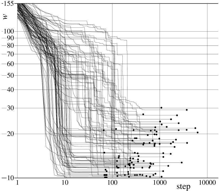
Figure 4: The effective weight $w=\|{\boldsymbol{\xi}}\|_{2}^{2}$ for $n_{\rm iter}=4$ decoder and the Tanner’s $[155,64,20]$ code vs. the number L2 line in Fig. 3 visits, i.e., the number of algorithm steps, $100$ realizations are shown.

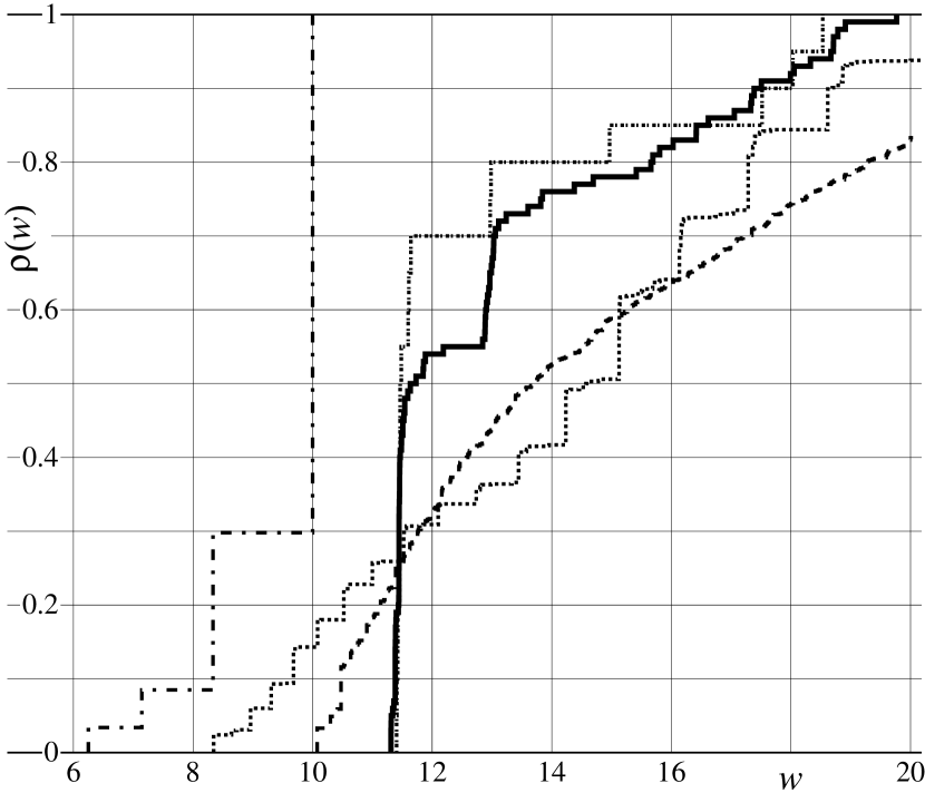
Figure 5: The probability/frequency of occurrence, $\rho(w)$, of the produced by the search algorithm in Fig. 3 instantons to have the weight $w$ or smaller, $n_{\rm iter}=2$, $3$, $4$, $10$, and $20$ (dash-dotted, dotted, dashed, solid, and fuzzy line, and $1000$, $1000$, $1000$, $100$, and $20$ realizations, respectively).

IV Instantons array

In this section the iterative decoder after each iteration checks the output ${\boldsymbol{\sigma}}=\operatorname{sign}{\boldsymbol{m}}$ for being a valid codeword, i.e., ${\hat{H}}\cdot\big{(}(1-{\boldsymbol{\sigma}})/2\big{)}={\boldsymbol{0}}~{}\mbox{(mod $2$)}$ (and if it is, the iterations stop).

Definition 3

The noise configuration is said to withstand $n$ iterations if for all $m\leq n$ the decoding output after $m$ iterations is wrong (that includes the case when the decoding stops before $n$ iterations). All such configurations form a set ${\cal E}(n)\subseteq{\bf R}^{N}$.

Statement 1

Checking for the output being a codeword at each iteration makes the set ${\cal E}$ being a non-increasing function of the number of iterations: ${\cal E}(n+1)\subseteq{\cal E}(n)$ for all $n$.

Proof:

Let ${\boldsymbol{\xi}}\notin{\cal E}(n)$, i.e., the decoding output at $n^{\rm th}$ [or earlier] iteration is the correct one. As it is a valid codeword, the decoding stops, and it will be the output of the decoding with any $n_{\rm iter}\geq n$ iterations, e.g., ${\boldsymbol{\xi}}\notin{\cal E}(n+1)$. ∎

In other words, an error of ${\sf W}$[rong] type is unrecoverable, as the decoding is stopped; otherwise doing more iterations could potentially result in the correct decoding.

Figure 6: Two-dimensional cuts of the [$155$-dimensional] noise space that contain zero noise vector ${\boldsymbol{0}}$ and the lowest weight instanton ${\boldsymbol{\xi}}_{\sf A}$ for Tanner’s $[155,64,20]$ code and AWGN channel. The line going through ${\boldsymbol{0}}$ and ${\boldsymbol{\xi}}_{\sf A}$ is horizontal. The plane of the cut is determined by the 3rd point it goes through. In panels (a), (b), and (c) it is the instanton ${\boldsymbol{\xi}}_{\sf B}$; in panel (d) it is a random vector; and in panel (e) it is the vector ${\boldsymbol{t}}$ with $t_{60}=t_{122}=t_{130}=t_{131}=t_{136}=1$ and all other components being $0$. The labels $0$, $1$, $2$, $3$, and $4$ indicate how many iterations the noise withstands in this area. The tone of gray is calculated as $(9-\log_{2}n)/11$, where $n$ is how many iterations the noise configuration withstands, with $0$/$1$ being black/white. Tones $10/11$ and $1$ correspond to $n=0$ and correct decoding without any iterations (i.e., $\xi_{i}<1$ for all $i$).

The problem of instanton-amoeba scheme [10, 11] for large number of iterations is with the rough landscape of the function amoeba tries to optimize. The moves amoeba does do assume that the landscape is regular (see [28, 29]). The problem with the application of downhill simplex/amoeba method to finding $n_{\rm iter}$ instantons is that amoeba always aims for noise configurations that withstand $n_{\rm iter}$ (i.e., many) iterations. The set ${\cal E}(n_{\rm iter})$ of such noise configurations [for large $n_{\rm iter}$] is very irregular near its boundary (see Fig. 6 and also [30]), and amoeba is getting confused and uncontrollably reduces its size without any progress.

L1	start with the noise vector ${\boldsymbol{\xi}}=(1,1,\dots,1)$
L2	check some (may be empty) list of noise vectors
L3	for $k=0$, $1$, …, $n_{\rm iter;max}$
L4	perturb ${\boldsymbol{\xi}}(k)$
L5	check perturbed noise vector
L6	go to L3 or exit

Figure 7: Iterative decoding instanton search algorithm.

Figure 8: The two lowest instantons ${\boldsymbol{\xi}}_{\sf A}$ and ${\boldsymbol{\xi}}_{\sf B}$. The tone of gray is calculated as $1-\xi/2$, with $\xi=2$ / $\xi=0$ being black/white. The $155\times 93$ parity check matrix ${\hat{H}}$ consists of three blocks: $({\hat{R}}^{1}~{}{\hat{R}}^{2}~{}{\hat{R}}^{4}~{}{\hat{R}}^{8}~{}{\hat{R}}^{16})$, $({\hat{R}}^{5},{\hat{R}}^{10}~{}{\hat{R}}^{20}~{}{\hat{R}}^{9}~{}{\hat{R}}^{18})$, $({\hat{R}}^{25}~{}{\hat{R}}^{19}~{}{\hat{R}}^{7}~{}{\hat{R}}^{14}~{}{\hat{R}}^{28})$, where ${\hat{R}}$ is the $31\times 31$ matrix that cyclically shifts a column vector up by one component.

Figure 9: Iterative decoding output ${\boldsymbol{m}}$ on the instantons ${\boldsymbol{\xi}}_{\sf A}$ and ${\boldsymbol{\xi}}_{\sf B}$, $200$ iterations running from top to bottom are shown. The tone of gray is calculated as $(1+m/10)/2$, with $0$/$1$ being black/white. Middle gray (tone $1/2$) corresponds to undecided output $m=0$. The decoding input ${\boldsymbol{h}}={\boldsymbol{m}}^{(0)}$ is shown at the top for comparison of input and output magnitudes.

The algorithm shown in Fig. 7 and described below overcomes this difficulty and is able to find instantons for large $n_{\rm iter}$. The procedure deals with the array of noise configurations, ${\boldsymbol{\xi}}(k)$, $k=0$, $1$, …, $n_{\rm iter;max}$, where at any time the noise ${\boldsymbol{\xi}}(k)$ is the one with the largest $P({\boldsymbol{\xi}})$ (or the lowest weight $w({\boldsymbol{\xi}})\propto\sum_{i=1}^{N}F(\xi_{i})$) from all the withstanding $k$ iterations noise configurations that were encountered in the procedure so far. (The updates of ${\boldsymbol{\xi}}(k)$ are done in the line L5 and (at the start) in the line L2.)

In the line L1 of the algorithm the output of the channel is completely undecided (${\boldsymbol{h}}=(0,0,\dots,0)$). This configuration obviously withstands $\infty$ iterations, although $P({\boldsymbol{\xi}})$ at it is quite low. This step makes ${\boldsymbol{\xi}}(k)=(1,1,\dots,1)$ for all $k=0$, $1$, …, $n_{\rm iter;max}$.

In the line L2 the noise configurations that are known from some external source (e.g., from previous runs of the procedure or from the analysis of trapping sets or pseudo-codewords) may be introduced as a starting point for instanton search.

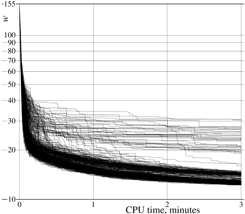
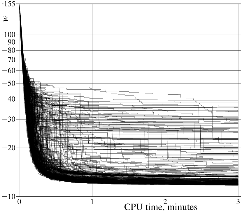
Figure 10: The effective weight $w$ of the withstanding $n_{\rm iter;max}=100$ iterations noise configuration for the Tanner’s $[155,64,20]$ code and AWGN channel vs. CPU (Intel Xeon X3360, $2.83~{}{\rm GHz}$) time, $500$ realizations are shown. The feedback for the amplitude $a$ is A (upper panel) and D (lower panel).

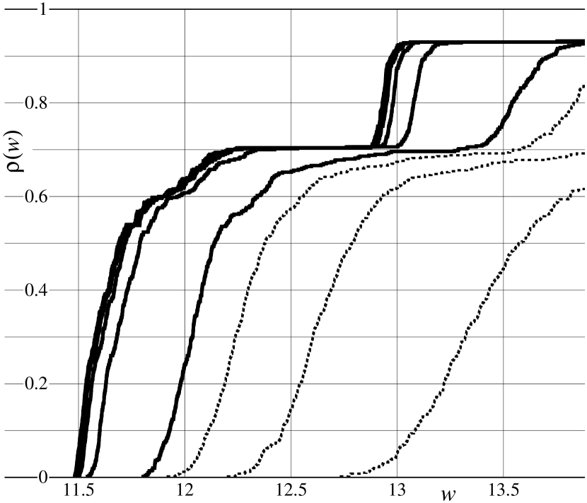
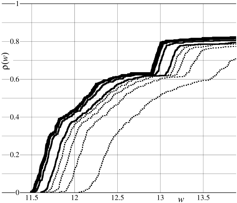
Figure 11: The probability/frequency of occurrence, $\rho(w)$, of the withstanding $n_{\rm iter;max}=100$ iterations noise configurations with the weight $w$ or smaller after $1$, $2$, $3$, $4$ (dashed curves) and $5$, $10$, …, $30$ (solid curves) minutes of CPU time. Code, channel, feedback, and CPU are the same as in Fig. 10.

This procedure, applied to Tanner’s $[155,64,20]$ code and AWGN channel, with $n_{\rm iter;max}=100$, produced an instanton ${\boldsymbol{\xi}}_{\sf A}$ with the lowest weight $w({\boldsymbol{\xi}}_{\sf A})=\|{\boldsymbol{\xi}}_{\sf A}\|_{2}^{2}<11.475333$ that causes iterations to cycle with the period of length $12$ (see Fig. 9). The next instanton ${\boldsymbol{\xi}}_{\sf B}$ has the weight $w({\boldsymbol{\xi}}_{\sf B})\approx 11.4996$. The differences in weight for configurations that withstand $20$ or more iterations are very small. Submitting the array ${\boldsymbol{\xi}}(k)$ as an initial state of the procedure with larger $n_{\rm iter;max}$ relatively quickly produces noise configurations with very close weight that withstand larger $n_{\rm iter;max}$ iterations.

Below are the details of the procedure used to generate Figs. 10 and 11. The noise vector ${\boldsymbol{\xi}}$ is perturbed as ${\boldsymbol{\xi}}\to c{\boldsymbol{\xi}}+a{\boldsymbol{\psi}}$, where the components of ${\boldsymbol{\psi}}$ are independent standard normal random variables. The coefficient $c=\sqrt{1-a^{2}N/w({\boldsymbol{\xi}})}<1$ makes the expected value ${\sf E}\,\|c{\boldsymbol{\xi}}+a{\boldsymbol{\psi}}\|_{2}^{2}=c^{2}w({\boldsymbol{\xi}})+a^{2}N=w({\boldsymbol{\xi}})$ not being systematically increased by the addition of $a{\boldsymbol{\psi}}$.

One doesn’t want to have the amplitude of the perturbation $a$ being too small (or the optimization is slow) or too large (then the perturbed noise is rejected often). To accelerate the procedure the amplitude $a$ is chosen according to the following negative feedback: Each noise configuration ${\boldsymbol{\xi}}$ has a number $A$ attached to it, and the perturbed noise $c{\boldsymbol{\xi}}+a{\boldsymbol{\psi}}$ gets the number $2A$ attached, while the number attached to ${\boldsymbol{\xi}}$ is decreased by a factor $0.999$. In the line L1 the value $A=0.1$ is attached. The amplitude of the perturbation $a$ is chosen as A: $a=A$; D: $0.1A<a<A$; and W: $10^{-14}<a<0.1$, with uniform distribution of $\log a$ in both D and W. In comparison to A and D, the progress in W is slow — the perturbation amplitude $a$ is often too small or too large.

How $w\big{(}{\boldsymbol{\xi}}(100)\big{)}$ goes down with time is shown in Fig. 10. It can be seen that sometimes $w\big{(}{\boldsymbol{\xi}}(100)\big{)}$ suddenly drops down quite a bit — it is happening when beginning part of the array (but not ${\boldsymbol{\xi}}(100)$) already went lower in weight, and then suddenly a small perturbation withstands $100$ iterations, so ${\boldsymbol{\xi}}(100)$ is updated. Such events are what makes the whole procedure work. The progress in the beginning part of the array is a lot more regular, and the procedure treasures it in hope that it will be converted into the progress at $n_{\rm iter;max}$.

The distribution of $w\big{(}{\boldsymbol{\xi}}(100)\big{)}$ is shown in Fig. 11. As it can be seen, the fate of the run is determined quite early.

At the very beginning there are few rejections of the perturbed noise vectors, and with the feedback A [with larger choices of $a$] the weight goes down faster than with D (see Fig. 10). When the weight reaches about $20$, the feedback D is more effective, probably because eventual smaller than $A$ choices of $a$ lead to the perturbations being not rejected more often, which keeps the values of $A$ large enough. Eventually A is more effective (see Fig. 11), although such a difference between A and D is a bit surprising.

V Discussion

The lowest instanton weight $w$ describes how fast the decoding error probability goes down with SNR in the high SNR limit: $\log P({\cal E})\sim-\beta({\rm SNR})\cdot w$. The value of $w$ quickly saturates with the number of iterations $n_{\rm iter}$, and the decrease of $P({\cal E})$ with $n_{\rm iter}$ is probably caused by the thinning of the set ${\cal E}(n_{\rm iter})$ in the vicinity of the instanton. How exactly does this happen?

In the vicinity of the instantons ${\boldsymbol{\xi}}_{\sf A}$ and ${\boldsymbol{\xi}}_{\sf B}$ there are noise configurations that withstand just $3$ iterations (see Fig. 6). Is it possible to locate these instantons from the analysis of the decoding with small number iterations?

In the example from Sec. II the magnitude of iterative decoder messages was growing linearly with the iteration number. Such a linear growth was not observed for the instantons ${\boldsymbol{\xi}}_{\sf A}$ and ${\boldsymbol{\xi}}_{\sf B}$. Should that be expected?

Let ${\rm CT}_{i}$ be the Computational Tree (CT) with $n_{\rm iter}$ generations that starts at the bit $i$; $X$ and ${\cal X}_{i}$ be the vector spaces of noise configurations on the original error correcting code and on ${\rm CT}_{i}$. For any noise configuration ${\boldsymbol{\xi}}\in X$ let us define the noise configuration ${\boldsymbol{\Xi}}={\rm CT}_{i}({{\boldsymbol{\xi}}})\in{\cal X}_{i}$ on the ${\rm CT}_{i}$ by making the value of ${\boldsymbol{\Xi}}$ on any copy of bit $j$ to be equal to $\xi_{j}$. This defines a linear mapping ${\rm CT}_{i}:X\to{\cal X}_{i}$.

Definition 4

A noise configuration ${\boldsymbol{\Xi}}$ on ${\rm CT}_{i}$ is called admissible if the noise values on different copies of the same bit are equal, i.e., ${\boldsymbol{\Xi}}={\rm CT}_{i}({\boldsymbol{\xi}})$ for some noise ${\boldsymbol{\xi}}$.

Consider some noise configuration ${\boldsymbol{\xi}}_{0}$ which causes a decoding error after $n_{\rm iter}$ iterations are done, i.e., ${\boldsymbol{\xi}}_{0}\in{\cal E}$. The goal is to generate lower weight noise ${\boldsymbol{\xi}}\in{\cal E}$.

For each bit $i$ let us denote the most probable pseudo-codewords (codewords on the CT that starts at bit $i$) with correct (“$+$”) and incorrect (“$-$”) values at the the central bit by ${\boldsymbol{\Sigma}}^{(i,\pm)}$. (Notice that ${\boldsymbol{\Sigma}}$, as a vector with components sitting on the CT bits, could have different values at different CT copies of initially the same bit of the code.) The whole CT structure of ${\boldsymbol{\Sigma}}^{(i,\pm)}$ is not going to be needed. As in [3], it will be enough to know for each bit $j$ the number $M_{j}^{(i,\pm)}$ of its copies in ${\rm CT}_{i}$ that have “$-$” value in ${\boldsymbol{\Sigma}}^{(i,\pm)}$. The pseudo-codewords ${\boldsymbol{\Sigma}}^{(i,\pm)}$ are then described by $N$-dimensional vectors ${\boldsymbol{M}}^{(i,\pm)}$.

Here is how the vectors ${\boldsymbol{M}}^{(i,\pm)}$ can be obtained by dynamic programming [31], propagating from the leaves of the tree to its center: Proceed with iterative decoding, but instead of standard log-likelihood messages send $N$-dimensional vectors containing numbers of “$-$” copies. Here are the exact formulas for the “decoding”:

$${\displaystyle\begin{array}[]{c}\raisebox{-1.0pt}{\mbox{bits $\to$ checks}}\\ \raisebox{1.0pt}{\mbox{messages}}\end{array}\!\!\!\!:} {\boldsymbol{\eta}}_{j\to\alpha}^{(k)}(\pm)={\textstyle\frac{1\mp 1}{2}}{\boldsymbol{e}}_{j}+\sum_{\beta\neq\alpha}^{j\circ\hskip-1.25pt-\hskip-1.7pt\raisebox{-0.8pt}{\scalebox{0.75}{\mbox{\rotatebox{45.0}{$\diamond$}}}}\beta}{\boldsymbol{\mu}}_{\beta\to j}^{(k-1/2)}(\pm)$$

$${\displaystyle\begin{array}[]{c}\raisebox{-1.0pt}{\mbox{checks $\to$ bits}}\\ \raisebox{1.0pt}{\mbox{messages}}\end{array}\!\!\!\!:} {\boldsymbol{\mu}}_{\alpha\to j}^{(k+1/2)}(\pm)=\sum_{l\neq j}^{l\circ\hskip-1.25pt-\hskip-1.7pt\raisebox{-0.8pt}{\scalebox{0.75}{\mbox{\rotatebox{45.0}{$\diamond$}}}}\alpha}{\boldsymbol{\eta}}_{l\to\alpha}^{(k)}(\sigma_{l})$$

$$\mathrlap{\mbox{~{}~{}~{}~{}where }\prod\limits_{l\neq j}^{l\circ\hskip-1.25pt-\hskip-1.7pt\raisebox{-0.8pt}{\scalebox{0.75}{\mbox{\rotatebox{45.0}{$\diamond$}}}}\alpha}\sigma_{l}=\pm\mbox{~{}~{}and~{}~{}}{\boldsymbol{h}}\,\cdot\!\sum_{l\neq j}^{l\circ\hskip-1.25pt-\hskip-1.7pt\raisebox{-0.8pt}{\scalebox{0.75}{\mbox{\rotatebox{45.0}{$\diamond$}}}}\alpha}{\boldsymbol{\eta}}_{l\to\alpha}^{(k)}(\sigma_{l})\mbox{ is minimal}}$$

decoding output: $${\boldsymbol{M}}^{(i,\pm)}={\textstyle\frac{1\mp 1}{2}}{\boldsymbol{e}}_{i}+\sum_{\alpha}^{i\circ\hskip-1.25pt-\hskip-1.7pt\raisebox{-0.8pt}{\scalebox{0.75}{\mbox{\rotatebox{45.0}{$\diamond$}}}}\alpha}{\boldsymbol{\mu}}_{\alpha\to i}^{(n_{\rm iter}-1/2)}(\pm)$$

Here ${\boldsymbol{e}}_{j}$ is the vector whose all but one components are equal to $0$, while its $j^{\rm\,th}$ component is equal to $1$. At the beginning of the decoding there are “no messages” to bits, i.e., ${\boldsymbol{\mu}}_{\alpha\to j}^{(-1/2)}(\pm)={\boldsymbol{0}}$ — the zero vector.

Another needed vector is ${\boldsymbol{N}}^{(i)}$ that contains the total number bits’ copies in the CT based on bit $i$:

$${\boldsymbol{\mu}}_{\alpha\to j}^{(-1/2)} ={\boldsymbol{0}} {\boldsymbol{\eta}}_{j\to\alpha}^{(k)} ={\boldsymbol{e}}_{j}+\sum_{\beta\neq\alpha}^{j\circ\hskip-1.25pt-\hskip-1.7pt\raisebox{-0.8pt}{\scalebox{0.75}{\mbox{\rotatebox{45.0}{$\diamond$}}}}\beta}{\boldsymbol{\mu}}_{\beta\to j}^{(k-1/2)}$$

$${\boldsymbol{\mu}}_{\alpha\to j}^{(k+1/2)} =\sum_{l\neq j}^{l\circ\hskip-1.25pt-\hskip-1.7pt\raisebox{-0.8pt}{\scalebox{0.75}{\mbox{\rotatebox{45.0}{$\diamond$}}}}\alpha}{\boldsymbol{\eta}}_{l\to\alpha}^{(k)} {\boldsymbol{N}}^{(i)} ={\boldsymbol{e}}_{i}+\sum_{\alpha}^{i\circ\hskip-1.25pt-\hskip-1.7pt\raisebox{-0.8pt}{\scalebox{0.75}{\mbox{\rotatebox{45.0}{$\diamond$}}}}\alpha}{\boldsymbol{\mu}}_{\alpha\to i}^{(n_{\rm iter}-1/2)}$$

From now on it is assumed that the transmission channel is the AWGN one, i.e., $h\propto(1-\xi)$.

Consider the case when the iterative decoding produces an error on bit $i$, i.e., $m^{(n_{\rm iter})}_{i}\leq 0$. Within ${\cal X}_{i}$ consider a sphere ${\cal S}_{i}$ with the center at ${\boldsymbol{\Xi}}_{0}:={\rm CT}_{i}({\boldsymbol{\xi}}_{0})$ and the radius $R_{i}:=\|{\boldsymbol{\Xi}}^{(i,+)}-{\boldsymbol{\Xi}}_{0}\|$, where ${\boldsymbol{\Xi}}^{(i,+)}:={\boldsymbol{1}}-{{\boldsymbol{\Sigma}}^{(i,+)}}$, and the vector ${\boldsymbol{1}}$ has all components being equal to $1$. All pseudo-codewords on the ${\rm CT}_{i}$ that have “$+$” at the center are outside of or on the sphere (as ${\boldsymbol{\Sigma}}^{(i,+)}$ is the most probable). As ${\boldsymbol{\xi}}_{0}$ causes a decoding error, the noise configuration ${\boldsymbol{\Xi}}^{(i,-)}:={\boldsymbol{1}}-{{\boldsymbol{\Sigma}}^{(i,-)}}$, that corresponds to the pseudo-codeword ${\boldsymbol{\Sigma}}^{(i,-)}$, is inside or on the sphere $\mathcal{S}_{i}$.

For brevity the mentioning of bit $i$ will be dropped from the notation ${\rm CT}_{i}$, ${\boldsymbol{N}}^{(i)}$, ${\boldsymbol{\Sigma}}^{(i,\pm)}$, $R_{i}$, etc.— the bit $i$ is fixed until we find the lower weight noise ${\boldsymbol{\xi}}$ with their knowledge. Such a procedure is repeated for all the bits $1\leq i\leq N$ on which the decoding is in error, and the lowest weight noise configuration found is kept.

The set of noise configurations on ${\rm CT}$ that are closer to ${\boldsymbol{\Xi}}^{(-)}$ than to the sphere $\mathcal{S}$ is the interior of a prolate spheroid with ${\boldsymbol{\Xi}}_{0}$ and ${\boldsymbol{\Xi}}^{(-)}$ as its foci.

The task is to find the admissible point ${\boldsymbol{\Xi}}={\rm CT}({\boldsymbol{\xi}})$ on the spheroid with the smallest weight $\|{\boldsymbol{\xi}}\|^{2}$. Let ${\boldsymbol{\Xi}}_{\mathcal{S}}$ be the point on the sphere ${\cal S}$ which is the closest to ${\rm CT}({\boldsymbol{\xi}})$. As ${\boldsymbol{\Xi}}_{0}={\rm CT}({\boldsymbol{\xi}}_{0})$ is the center of the sphere, we have ${\rm CT}({\boldsymbol{\xi}})=(1-\tau){\rm CT}({\boldsymbol{\xi}}_{0})+\tau{\boldsymbol{\Xi}}_{\cal S}$ with $0\leq\tau\leq 1$, so ${\boldsymbol{\Xi}}_{\cal S}$ is actually admissible and is generated by some noise ${\boldsymbol{\xi}}_{\cal S}$, i.e., ${\boldsymbol{\Xi}}_{\cal S}={\rm CT}({\boldsymbol{\xi}}_{\cal S})$.

Let us minimize the weight $\|{\boldsymbol{\xi}}\|^{2}$ adding the two constraints $\|{\boldsymbol{\Xi}}_{\mathcal{S}}-{\boldsymbol{\Xi}}_{0}\|=\|{\boldsymbol{\Xi}}^{(+)}-{\boldsymbol{\Xi}}_{0}\|$ and $\|{\boldsymbol{\Xi}}_{\cal S}-{\boldsymbol{\Xi}}\|=\|{\boldsymbol{\Xi}}^{(-)}-{\boldsymbol{\Xi}}\|$ using Lagrange multipliers $\lambda$ and $\mu$, respectively:

$$\mathcal{F}({\boldsymbol{\xi}}):=\|{\boldsymbol{\xi}}\|^{2} +\lambda\bigl{(}\|{\boldsymbol{\Xi}}-{\boldsymbol{\Xi}}_{0}\|^{2}-\tau^{2}R^{2}\bigr{)}$$

$$+\mu\bigl{(}\|{\boldsymbol{\Xi}}-{\boldsymbol{\Xi}}^{(-)}\|^{2}-(1-\tau)^{2}R^{2}\bigr{)}$$

$$R^{2}=\sum_{k=1}^{N}N_{k}\xi_{0k}^{2} +4\sum_{k=1}^{N}M^{(+)}_{k}(1-\xi_{0k})$$

Here the vector ${\boldsymbol{\xi}}_{\mathcal{S}}$ is already substituted by $\bigl{(}{\boldsymbol{\xi}}-(1-\tau){\boldsymbol{\xi}}_{0}\bigr{)}/\tau={\boldsymbol{\xi}}_{0}+({\boldsymbol{\xi}}-{\boldsymbol{\xi}}_{0})/\tau$. Varying over $\tau$ tests different “latitudes” on the spheroid and gives $\lambda\tau=\mu(1-\tau)$. Optimizing the quadratic function of ${\boldsymbol{\xi}}$, one gets ($\gamma:=\tau/\mu$)

$$\xi_{k}=\frac{\lambda N_{k}\xi_{0k}+2\mu M^{(-)}_{k}}{(\lambda+\mu)N_{k}+1}=\frac{(1-\tau)N_{k}\xi_{0k}+2\tau M^{(-)}_{k}}{N_{k}+\gamma}$$

In order to satisfy the two constraints, one must have

$$\sum_{k=1}^{N}N_{k}(\xi_{k}-\xi_{0k})^{2}=\tau^{2}R^{2}$$

$$\sum_{k=1}^{N}N_{k}\xi_{k}^{2}+4\sum_{k=1}^{N}M^{(-)}_{k}(1-\xi_{k})=(1-\tau)^{2}R^{2}$$

Subtracting one equation from another one gets a linear condition on ${\boldsymbol{\xi}}$ (and consequently on $\tau$), which allows to express the parameter $\tau$ through the rest:

$$\tau=\frac{\displaystyle\sum_{k=1}^{N}\biggl{[}\frac{2\gamma N_{k}\xi_{0k}^{2}}{N_{k}+\gamma}+4M^{(+)}_{k}(1-\xi_{0k})-4M^{(-)}_{k}\Bigl{(}1-\frac{N_{k}\xi_{0k}}{N_{k}+\gamma}\Bigr{)}\biggr{]}}{\displaystyle\sum_{k=1}^{N}\biggl{[}\frac{2\gamma N_{k}\xi_{0k}^{2}}{N_{k}+\gamma}+8M^{(+)}_{k}(1-\xi_{0k})-8M^{(-)}_{k}\frac{M^{(-)}_{k}-N_{k}\xi_{0k}}{N_{k}+\gamma}\biggr{]}}$$

The only remained parameter to find is $\gamma$, as $\tau$ is readily exppressed trough it. The task of finding the lowest weight noise ${\boldsymbol{\xi}}$ on the spheroid is reduced to finding the root of a single variable function.

In practice we expect a hypothetical instanton search procedure to quickly end up with $m^{(n_{\rm iter})}=0$, which means that ${\boldsymbol{\Xi}}^{(-)}$ lies on the sphere $\mathcal{S}$. The spheroid then degenerates into a segment connecting ${\boldsymbol{\Xi}}_{0}$ and ${\boldsymbol{\Xi}}^{(-)}$. Unless ${\boldsymbol{\Xi}}^{(-)}={\boldsymbol{1}}-{\boldsymbol{\Sigma}}^{(-)}$ is admissible, the optimization will end up in ${\boldsymbol{\xi}}={\boldsymbol{\xi}}_{0}$, i.e., no progress will be made. Such an unwanted situation is a result of dealing with the sphere $\mathcal{S}$, as we don’t know where other pseudo-codewords on ${\rm CT}$ with “+” value at the cental bit could lie — by dynamic programming we only did obtain ${\boldsymbol{\Sigma}}^{(+)}$.

References

[1]
R. G. Gallager, Low Density Parity Check Codes. Cambridge, MA: M.I.T. Press, 1963.
[2]
D. J. C. MacKay and R. M. Neal, “Near Shannon limit performance of low
density parity check codes,” Electron. Lett., vol. 32, no. 18, p.
1645, 1996.
[3]
N. Wiberg, “Codes and decoding on general graphs,” Ph.D. thesis, Univ.
Linköping, Sweden, 1996.
[4]
D. J. C. MacKay and M. S. Postol, “Weaknesses of Margulis and
Ramanujan–Margulis low-density parity-check codes,” Electronic
Notes in Theoretical Computer Science, vol. 74, pp. 97–104, 2003.
[5]
T. J. Richardson, “Error floors of LDPC codes,” in 41st Allerton
Conf. Commun., Control and Computing, (Monticello, IL, USA, October 1–3,
2003), pp. 1426–1435.
[6]
C. Di, D. Proietti, I. E. Telatar, T. J. Richardson, and R. L. Urbanke,
“Finite length analysis of low-density parity-check codes on the binary
erasure channel,” IEEE Trans. Inf. Theory, vol. 48, no. 6, pp.
1570–1579, 2002.
[7]
C. Kelley and D. Sridhara, “Pseudocodewords of Tanner graphs,” IEEE
Trans. Inf. Theory, vol. 53, no. 11, pp. 4013–4038, 2007.
[8]
J. Feldman, M. J. Wainwright, and D. R. Karger, “Using linear programming to
decode binary linear codes,” IEEE Trans. Inf. Theory, vol. 51, no. 3,
pp. 954–972, 2005.
[9]
Z. Zhang, L. Dolecek, B. Nikolić, V. Anantharam, and M. J. Wainwright,
“Design of LDPC decoders for improved low error rate performance:
quantization and algorithm choices,” IEEE Trans. Commun., vol. 57,
no. 11, pp. 3258–3268, 2009.
[10]
M. G. Stepanov, V. Chernyak, M. Chertkov, and B. Vasic, “Diagnosis of
weaknesses in modern error correction codes: a physics approach,”
Phys. Rev. Lett., vol. 95, no. 22, p. 228701, 2005.
[11]
M. G. Stepanov and M. Chertkov, “Instanton analysis of low-density
parity-check codes in the error-floor regime,” in 2006 IEEE Intl.
Symp. Inf. Theory, (Seattle, WA, USA, July 9–14, 2006), pp. 552–556.
[12]
R. M. Tanner, “A recursive approach to low complexity codes,” IEEE
Trans. Inform. Theory, vol. 27, no. 5, pp. 533–547, 1981.
[13]
B. Vasic, S. K. Chilappagari, D. V. Nguyen, and S. K. Planjery, “Trapping set
ontology,” in 47th Annual Allerton Conf. on Communications, Control
and Computing, (Monticello, IL, USA, September 30–October 2, 2009).
[14]
L. Dolecek, Z. Zhang, V. Anantharam, M. J. Wainwright, and B. Nikolić,
“Analysis of absorbing sets and fully absorbing sets of array-based LDPC
codes,” IEEE Trans. Inf. Theory, vol. 56, no. 1, pp. 181–201, 2010.
[15]
M. Karimi and A. H. Banihashemi, “Efficient algorithm for finding dominant
trapping sets of LDPC codes,” IEEE Trans. Inf. Theory, vol. 58,
no. 11, pp. 6942–6958, 2012.
[16]
J. Guo, J. Mu, X. Jiao, and G. Li, “Finding small fundamental instantons of
LDPC codes by path extension,” IEICE Trans. Fundamentals, vol.
E97-A, no. 4, pp. 1001–1004, 2014.
[17]
X. Liu and S. C. Draper, “The ADMM penalized decoder for LDPC codes,”
IEEE Trans. Inf. Theory, vol. 62, no. 6, pp. 2966–2984, 2016.
[18]
J. S. Yedidia, W. T. Freeman, and Y. Weiss, “Constructing free-energy
approximations and generalized belief propagation algorithms,” IEEE
Trans. Inf. Theory, vol. 51, no. 7, pp. 2282–2312, 2005.
[19]
J. Pearl, Probabilistic reasoning in intelligent systems: network of
plausible inference. San Francisco:
Kaufmann, 1988.
[20]
D. J. C. MacKay, “Good error-correcting codes based on very sparse matrices,”
IEEE Trans. Inf. Theory, vol. 45, no. 2, pp. 399–431, 1999.
[21]
S. C. Tatikonda and M. I. Jordan, “Loopy belief propagation and Gibbs
measures,” in 18th Conf. Uncertainty in Artificial Intelligence,
(Edmonton, AB, Canada, August 1–4, 2002), pp. 493–500.
[22]
T. Heskes, “On the uniqueness of loopy belief propagation fixed points,”
Neural Computation, vol. 16, no. 11, pp. 2379–2413, 2004.
[23]
R. M. Tanner, D. Sridhara, and T. Fuja, “A class of group-structured LDPC
codes,” in 6th Intl. Symp. Commun. Theory Appl., (Ambleside, UK, July
15–20, 2001).
[24]
R. Koetter and P. O. Vontobel, “Graph covers and iterative decoding of
finite-length codes,” in 3rd Intl. Conf. Turbo Codes and Related
Topics, (Brest, France, September 1–5, 2003), pp. 75–82.
[25]
M. Chertkov and M. G. Stepanov, “An efficient pseudocodeword search algorithm
for linear programming decoding of LDPC codes,” IEEE Trans. Inf.
Theory, vol. 54, no. 4, pp. 1514–1520, 2008.
[26]
A. Lifshitz and Y. Beéry, “On pseudocodewords and decision regions of linear
programming decoding of HDPC codes,” IEEE Trans. Commun., vol. 60,
no. 4, pp. 963–971, 2012.
[27]
M. Chertkov and M. Stepanov, “Polytope of correct (linear programming)
decoding and low-weight pseudo-codewords,” in 2011 IEEE Intl. Symp.
Inf. Theory, (St. Petersburg, Russia, July 31–August 5, 2011), pp.
1648–1652.
[28]
J. A. Nelder and R. Mead, “A simplex method for function minimization,”
Computer Journal, vol. 7, no. 4, pp. 308–313, 1965.
[29]
W. H. Press, S. A. Teukolsky, W. T. Vetterling, and B. P. Flannery,
Numerical recipes in C: the art of scientific computing. Cambridge: Cambridge University Press, 1988.
[30]
P. O. Vontobel and R. Koetter, “Graph covers and iterative decoding of
finite-length codes,” in DIMACS Workshop on Algebraic Coding Theory
and Information Theory, (Piscataway, NJ, USA, December 15–18, 2003).
[31]
R. E. Bellman, Dynamic programming. Princeton, NJ: Princeton University Press, 1957, (reprinted:
Dover Publications, 2003).