Anderson Orthogonality in the Dynamics After a Local Quantum Quench

Abstract

We present a systematic study of the role of Anderson orthogonality for the dynamics after a quantum quench in quantum impurity models, using the numerical renormalization group. As shown by Anderson in 1967, the scattering phase shifts of the single-particle wave functions constituting the Fermi sea have to adjust in response to the sudden change in the local parameters of the Hamiltonian, causing the initial and final ground states to be orthogonal. This so-called Anderson orthogonality catastrophe also influences dynamical properties, such as spectral functions. Their low-frequency behaviour shows nontrivial power laws, with exponents that can be understood using a generalization of simple arguments introduced by Hopfield and others for the X-ray edge singularity problem. The goal of this work is to formulate these generalized rules, as well as to numerically illustrate them for quantum quenches in impurity models involving local interactions. As a simple yet instructive example, we use the interacting resonant level model as testing ground for our generalized Hopfield rule. We then analyse a model exhibiting population switching between two dot levels as a function of gate voltage, probed by a local Coulomb interaction with an additional lead serving as charge sensor. We confirm a recent prediction that charge sensing can induce a quantum phase transition for this system, causing the population switch to become abrupt. We elucidate the role of Anderson orthogonality for this effect by explicitly calculating the relevant orthogonality exponents.

I Introduction

The Anderson orthogonality (AO) catastrophe Anderson1967 refers to the response of a Fermi sea to a change in a local scattering potential, described, say, by a change in Hamiltonian from $\hat{H}_{\rm i}$ to $\hat{H}_{\rm f}$. Such a change induces changes in the scattering phase shifts of all single-particle wave functions. This causes the initial ground state $|G_{\rm i}\rangle$ of $\hat{H}_{\rm i}$ and the final ground state $|G_{\rm f}\rangle$ of $\hat{H}_{\rm f}$, both describing a filled Fermi sea but w.r.t. different single-particle wave functions, to be orthogonal in the thermodynamic limit, even if the changes in the single-particle wave functions are minute. The overlap of the respective ground states scales as Anderson1967 ; Schotte1969

$$|\langle G_{\rm i}|G_{\rm f}\rangle|\sim N^{-\frac{1}{2}\Delta_{\rm AO}^{2}}\>,$$ (1)

where $N$ is the number of particles in the system, and the exponent $\Delta_{\rm AO}$ characterizes the degree of orthogonality.

AO underlies the physics of numerous dynamical phenomena such as the Fermi edge singularity, Mahan1967 ; Schotte1969 ; Hopfield1969 ; Nozieres the Altshuler-Aronov zero bias anomaly Altshuler1979 in disordered conductors, tunnelling into strongly interacting Luttinger liquids, Gogolin1993 ; Prokofev1994 ; Affleck1994 ; Furusaki1997 ; Gogolin slow relaxation in electron glasses, Leggett1987 ; Ovadyahu2007 and optical absorption involving a Kondo exciton,Helmes2005 ; Tureci2011 ; Latta2011 where photon absorption induces a local quantum quench, to name but a few. Recently, AO has also been evoked Goldstein2010 ; Goldstein2011 in an analysis of population switching (PS) in quantum dots (the fact that the population of individual levels of a quantum dot may vary non-monotonically with the gate voltage), and was argued to lead, under certain conditions involving a local Coulomb interaction with a nearby charge sensor, to a quantum phase transition.

One of the goals of the present work is to analyse the latter prediction in quantitative detail. Another is to generalize arguments that were given in Refs. Helmes2005, ; Tureci2011, ; Latta2011, , for the role of AO for spectral functions of the excitonic Anderson model, to related models with a similar structure. Thus, we present a systematic study of the role of Anderson orthogonality for the dynamics after a quantum quench in quantum impurity models involving local interactions, using the numerical renormalization group (NRG).Wilson1975 ; Bulla2008 We thereby extend a recent study, Weichselbaum2011 which showed how $\Delta_{\rm AO}$ can be calculated very accurately (with errors below $1\%$) by using NRG to directly evaluate overlaps such as $\langle G_{\rm i}|G_{\rm f}\rangle$, to the domain of dynamical quantities.

The spectral functions that characterize a local quantum quench typically show power-law behaviour, ${\sim\omega^{-1+2\eta}}$, in the limit of small frequencies, where $\eta$ typically depends on $\Delta_{\rm AO}$.Mahan1967 ; Schotte1969 ; Hopfield1969 ; Nozieres For the case of the X-ray edge singularity, Hopfield Hopfield1969 gave a simple argument to explain the relation between $\Delta_{\rm AO}$ and $\eta$. We frame Hopfield’s argument in a more general setting and numerically illustrate the validity of the resulting generalized Hopfield rule (Eq. (25) below) for several nontrivial models. In particular, we also analyse how this power-law behaviour is modified at low frequencies when one adds to the Hamiltonian an extra tunnelling term, that describes transitions between the Hilbert spaces characterizing the “initial” and “final” configurations. This effect plays a crucial role in understanding the abovementioned quantum phase transition for population switching.

The paper is organized as follows. In Sec. II we review various consequences of AO in different but related settings, and formulate the abovementioned generalization of Hopfield’s rule. In Sec. III we illustrate this rule for the spinless interacting resonant level model (IRLM), involving a single localized level interacting with the Fermi sea of a single lead. We consider this model without and with tunnelling, and study a quantum quench of the energy of its local level, focussing on signatures of AO in each case. Finally, in Sec. IV and Sec. V we discuss population switching without and with a charge sensor, respectively, confirming that if the sensor is sufficiently strongly coupled, AO indeed does cause population switching to become a sharp quantum phase transition. Section VI offers concluding remarks and outlines prospective applications of the present analysis.

II Various Consequences of Anderson Orthogonality

In this section we review various consequences of AO, in different but related settings. We begin by recalling two well-known facts: first, the relation between the exponent $\Delta_{\rm AO}$ and the charge that is displaced due to the quantum quench, $\Delta_{\rm ch}$; and second, the role of $\Delta_{\rm AO}$ in determining the asymptotic long-time power-law decay of correlation functions $\mathcal{G}_{X}(t)$ involving an operator $\hat{X}^{\dagger}$ that connects the initial and final ground state.

Then we consider the spectral function $\mathcal{A}_{X}(\omega)$ associated with $\mathcal{G}_{X}(t)$, which correspondingly shows asymptotic power-law behaviour, ${\sim\omega^{-1+2\eta}}$, for small frequencies, where the exponent $\eta$ depends on $\Delta_{\rm AO}$. We recall and generalize an argument due to Hopfield, that extends the relation between $\eta$ and $\Delta_{\rm AO}$ to composite local operators. Finally, we recapitulate how all these quantities can be calculated using NRG.

For simplicity, we assume in most of this section that the Fermi sea consists only of a single species of (spinless) electrons.The generalization to several channels needed in subsequent sections (in particular for discussing PS), is straightforward and will be introduced later as needed.

Although the concepts summarized in subsections II.2 to II.5 below apply quite generically to a wide range of impurity models, for definiteness we will illustrate them by referring to a particularly simple example, to be called the “local charge model” (LCM), which we define next.

II.1 Local charge model

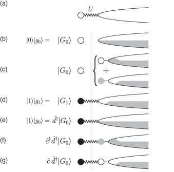
Figure 1: (a) Cartoon of the Hamiltonian (2) for the LCM. (b) to (g) Cartoons of the occupation of the dot and a half-filled lead, for $U>0$, for several states discussed in the text. (b) and (c) give two equivalent depictions of the ground state $|G_{0}\rangle$ of $\hat{H}_{0}$. (c) depicts the fact that $|g_{0}\rangle$ can be written as a superposition of the form $|0\rangle_{\rm c}|Q\rangle_{\rm rest}+|1\rangle_{\rm c}|Q-1\rangle_{\rm rest}$, indicating complementary occupations of the first site and the rest of a half-filled Wilson chain (defined in Sec. II.5 below). Here $|0\rangle_{\rm c}$ (which obeys $\hat{c}|0\rangle_{\rm c}=0$) and $|1\rangle_{\rm c}=\hat{c}^{\dagger}|0\rangle_{\rm c}$ describe the first site of the Wilson chain being empty or filled, respectively; the charge in the rest of the Wilson chain is correspondingly distributed in such a way that both components of the superposition have the same total charge, $Q$. (d) depicts the ground state $|G_{1}\rangle$ of $\hat{H}_{1}$, indicating that charge on the dot pushes charge in the lead away from the dot site. (e) shows the effect of applying $\hat{d}^{\dagger}$ to $|G_{0}\rangle$, the latter depicted according to (b). Similarly, (f) and (g) show the effect of applying $\hat{c}^{\dagger}\hat{d}^{\dagger}$ or $\hat{c}\hat{d}^{\dagger}$ to $|G_{0}\rangle$, the latter depicted according to (c). The displaced charge flowing inwards from infinity towards the dot as each of the states (e) to (g) evolves to the final ground state $|G_{1}\rangle$ of (d) is $\Delta_{d}<0$, $\Delta_{d}-1<0$ or $\Delta_{d}+1>0$, respectively. Comparison of (f) and (g) with (e) shows average charge differences of $+1$ and $-1$, respectively, in accord with the Hopfield-type argument summarized by Eq. (15).

The LCM describes a single spinless localized level, to be called dot level (alluding to a localized level in a quantum dot), interacting with a single Fermi sea of spinless electrons [see Fig. 1(a)]:

$$\hat{H}_{\rm LCM}(\hat{n}_{d})=U\,\hat{n}_{d}\,\hat{c}^{\dagger}\hat{c}+\sum_{\varepsilon}\varepsilon\,\hat{c}_{\varepsilon}^{\dagger}\hat{c}_{\varepsilon}^{{\phantom{\dagger}}}\>.$$ (2)

Here $\hat{c}_{\varepsilon}^{{\phantom{\dagger}}}$ and $\hat{d}$ are annihilation operators for Fermi sea states and the dot state, respectively, $\hat{n}_{d}=\hat{d}^{\dagger}\hat{d}$ counts the number of dot electrons, and $\hat{c}\equiv\hat{\psi}(0)\equiv\sum_{\varepsilon}\hat{c}_{\varepsilon}^{{\phantom{\dagger}}}$ destroys a Fermi sea electron at the position of the dot. The interaction is taken to be repulsive, $U>0$. There is no tunnelling between dot and sea. Therefore, the Hilbert space separates into two distinct sectors, in which the local charge operator $\hat{n}_{d}$ has eigenvalues $n_{d}=0$ and $n_{d}=1$, respectively. The Hamiltonians describing the Fermi sea in the two distinct sectors are

$$\hat{H}_{0} = \hat{H}_{\rm LCM}(n_{d}=0)=\sum_{\varepsilon}\varepsilon\,\hat{c}_{\varepsilon}^{\dagger}\hat{c}_{\varepsilon}^{{\phantom{\dagger}}}\>,$$ (3a)

$$\hat{H}_{1}(U) = \hat{H}_{\rm LCM}(n_{d}=1)=\sum_{\varepsilon}\varepsilon\,\hat{c}_{\varepsilon}^{\dagger}\hat{c}_{\varepsilon}^{{\phantom{\dagger}}}+U\hat{c}^{\dagger}\hat{c}\>.\qquad\phantom{.}$$ (3b)

We will denote their respective ground states [illustrated in Figs. 1(b,c) and 1(d), respectively] by

$$|G_{0}\rangle=|0\rangle|g_{0}\rangle\>,\qquad|G_{1}\rangle=|1\rangle|g_{1}\rangle\>,$$ (4)

where $|0\rangle$ and $|1\rangle=\hat{d}^{\dagger}|0\rangle$ describe the dot state with charge 0 or 1, respectively, and $|g_{0}\rangle$ and $|g_{1}\rangle$ the corresponding Fermi sea ground states.

The LCM contains all ingredients needed for AO, hence we will repeatedly refer to it below as an explicit example of the general arguments to be presented. [Corresponding LCM passages will sometimes appear in square brackets, so as not to disrupt the general flow of the discussion.] Explicit numerical results for the LCM will be presented in Sec. III.1 below.

II.2 AO and the displaced charge

For the ensuing discussions, it will be useful to distinguish between two types of quenches, to be called type 1 and 2, which we now discuss in turn.

Type 1 quench: For a type 1 quench, some parameter of the Hamiltonian is changed abruptly (e.g. by a sudden change of gate voltage for one of the gates defining a quantum dot). Taking the LCM as an example, suppose that the value of the interaction in the LCM is changed suddenly from $U$ to $U^{\prime}$ for a fixed local charge of $n_{d}=1$. This corresponds to a type 1 quench with

$$\hat{H}_{\rm i} =\hat{H}_{1}(U)\,,\quad \hat{H}_{\rm f} =\hat{H}_{1}(U^{\prime})\,,$$ (5a)

$$|G_{{\rm i}}\rangle =|1\rangle|g_{1,{\rm i}}\rangle\,,\quad |G_{{\rm f}}\rangle =|1\rangle|g_{1,{\rm f}}\rangle\,.\phantom{(}$$ (5b)

The overlap of initial and final ground states,

$$|\langle G_{{\rm i}}|G_{{\rm f}}\rangle|=|\langle g_{1,{\rm i}}|g_{1,{\rm f}}\rangle|\sim N^{-\frac{1}{2}\Delta_{\rm AO}^{2}}\>,$$ (6)

will vanish in the thermodynamic limit due to AO, since the two Fermi sea states $|g_{1,{\rm i}}\rangle$ and $|g_{1,{\rm f}}\rangle$ feel scattering potentials of different strengths.

In his classic 1967 paper, Anderson showed that for this type of situation the exponent $\Delta_{\rm AO}$ in Eq. (6) is equal to the change in scattering phase shifts at the Fermi surface divided by $\pi$, in reaction to the change in the strength of the scattering potential. According to the Friedel sum rule, Friedel1952 ; Friedel1956 ; Langreth1966 ; Hewson the change in phase shifts divided by $\pi$, in turn, is equal to the displaced charge $\Delta_{\rm ch}$ (in units of $e$) that flows inward from infinity into a large but finite volume (say $V_{\rm large}$) surrounding the scattering site, in reaction to the change in scattering potential, so that $\Delta_{\rm AO}=\Delta_{\rm ch}$. To be explicit,

$$\Delta_{\rm ch}\equiv\langle G_{{\rm f}}|\hat{n}_{\rm tot}|G_{{\rm f}}\rangle-\langle G_{{\rm i}}|\hat{n}_{\rm tot}|G_{{\rm i}}\rangle\;,$$ (7)

where $\hat{n}_{\rm tot}\equiv\hat{n}_{\rm sea}+n_{\rm dot}$ counts the total number of electrons within $V_{\rm large}$, with $\hat{n}_{{\rm sea}}$ counting the Fermi sea electrons and $\hat{n}_{{\rm dot}}$ counting the electrons on the dot. [For the LCM, $\hat{n}_{{\rm dot}}=\hat{n}_{d}$.]

The relative sign between $\Delta_{\rm AO}$ and $\Delta_{\rm ch}$ ($+$ not $-$) is a matter of convention, which does not affect the orthogonality exponent $\Delta_{\rm AO}^{2}$. Our convention,Weichselbaum2011 which agrees with standard usage, StandardUsage is such that $\Delta_{\rm AO}>0$ (or $<0$) if the change in local potential induces electrons to flow inward toward (outward away from) the scattering site.

For the LCM quench of Eq. (5) above, the initial and final states have the same dot charge, $n_{d}=1$, hence the displaced charge reduces to $\Delta_{\rm ch}\equiv\langle g_{1,{\rm f}}|\hat{n}_{{\rm sea}}|g_{1,{\rm f}}\rangle-\langle g_{1,{\rm i}}|\hat{n}_{{\rm sea}}|g_{1,{\rm i}}\rangle$. However, such a simplification will not occur for more complex impurity models involving tunneling between dot and lead [of the form $(\hat{d}^{\dagger}\hat{c}+\hat{c}^{\dagger}\hat{d})$], so that the local charge is not conserved. Examples are the interacting resonant level model [Eq. (III.2) below], or the single-impurity Anderson model [Eq. (IV.1) below].

For such a model, consider a type 1 quench from $\hat{H}_{\rm i}$ to $\hat{H}_{\rm f}$, implemented by a sudden change in one or several model parameters, in analogy to Eq. (5a). Although the corresponding ground states $|G_{{\rm i}}\rangle$ and $|G_{{\rm f}}\rangle$ will no longer have the simple factorized form of Eq. (5b), they will still exhibit AO as in Eq. (1). Moreover, the decay exponent is still equal to the displaced charge, $\Delta_{\rm AO}=\Delta_{\rm ch}$, given by Eq. (7). (For a NRG verification of this fact, see Ref. Weichselbaum2011, .)

Type 2 quench: For a type 2 quench, all model parameters are kept constant, but the system is switched suddenly between two dynamically disconnected sectors of Hilbert space characterized by different conserved quantum numbers. Taking again the LCM of Eq. (2) as an example, suppose that the local charge is suddenly changed, say from $n_{d}=0$ to $1$, while all model parameters are kept constant. This corresponds to a type 2 quench with

$$\hat{H}_{\rm i} =\hat{H}_{0}\phantom{U}\,\quad \hat{H}_{\rm f} =\hat{H}_{1}\;,\phantom{U}\quad\phantom{.}$$ (8a)

$$|G_{\rm i}\rangle =|0\rangle|g_{0}\rangle,\quad |G_{\rm f}\rangle =|1\rangle|g_{1}\rangle.\quad\phantom{.}$$ (8b)

A physical example of such a quench would be core level X-ray photoemission spectroscopy (XPS), where an incident X-ray photon is absorbed by an atom in a crystal, accompanied by the ejection of a core electron from the material. Gunnarsson1983a This amounts to the sudden creation of a core hole, which subsequently interacts with the Fermi sea of mobile conduction electrons (but does not hybridize with them). Thus, in this example $\hat{n}_{d}$ would represent the hole number operator $\hat{n}_{h}=\hat{h}^{\dagger}\hat{h}$.

More generally, a type 2 quench presupposes a Hamiltonian $\hat{H}(\hat{n}_{x})$ that depends on a conserved charge, say $\hat{n}_{x}$ [such as $\hat{n}_{d}$ for the LCM], with eigenvalues $n_{x}$ [such as $n_{d}=0$ or $1$]. The Hilbert space can then be decomposed into distinct, dynamically disconnected sectors, labelled by $n_{x}$ and governed by effective Hamiltonians $\hat{H}(n_{x})$, whose ground states have the form $|G(n_{x})\rangle=|n_{x}\rangle|g(n_{x})\rangle$. A type 2 quench is induced by an operator, say $\hat{X}^{\dagger}$ [such as $\hat{d}^{\dagger}$ for the LCM], whose action changes the conserved charge, thereby connecting two distinct sectors, say $\langle n^{\prime}_{x}|\hat{X}^{\dagger}|n_{x}\rangle=1$, with $n^{\prime}_{x}\neq n_{x}$. For such a quench we make the identifications

$$\hat{H}_{\rm i} =\hat{H}(n_{x})\,\quad \hat{H}_{\rm f} =\hat{H}(n^{\prime}_{x})\,,\phantom{|n_{x}\rangle}\quad\phantom{.}$$ (9a)

$$|G_{\rm i}\rangle =|n_{x}\rangle|g(n_{x})\rangle,\quad |G_{\rm f}\rangle =|n_{x}^{\prime}\rangle|g(n_{x}^{\prime})\rangle.\quad\phantom{.}$$ (9b)

The overlap $\langle G_{{\rm i}}|G_{{\rm f}}\rangle=0$ vanishes trivially, because $\langle n_{x}|n_{x}^{\prime}\rangle=0$. However, define

$$|\psi_{{\rm i}}\rangle\equiv\hat{X}^{\dagger}|G_{\rm i}\rangle$$ (10)

to be the “initial post-quench state” obtained by the action of the charge switching operator $\hat{X}^{\dagger}$ on the initial ground state. [Fig. 1(e) illustrates this state for the LCM with $\hat{X}^{\dagger}=\hat{d}^{\dagger}$.] Then the overlap

$$\mathcal{O}_{X}\equiv|\langle\psi_{{\rm i}}|G_{{\rm f}}\rangle|=|\langle g(n_{x})|g(n_{x}^{\prime})\rangle|\sim N^{-\frac{1}{2}\Delta_{\!X}^{2}}$$ (11)

again shows AO, since it is equal to the overlap of two Fermi sea ground states corresponding to different local charges. The corresponding exponent in Eq. (11) can again be related to a displaced charge, $\Delta_{\!X}=\Delta_{\!X}^{{\rm ch}}$, but now the latter should compare the total charge within $V_{\rm large}$ described by the states $|G_{\rm f}\rangle$ and $|\psi_{{\rm i}}\rangle$:

$$\Delta_{\!X}^{{\rm ch}}\equiv\langle G_{{\rm f}}|\hat{n}_{{\rm tot}}|G_{{\rm f}}\rangle-\langle\psi_{{\rm i}}|\hat{n}_{\rm tot}|\psi_{{\rm i}}\rangle\>.$$ (12)

$\Delta_{\!X}^{{\rm ch}}$ can be interpreted as the charge (in units of $e$) that flows into $V_{\rm large}$ during the post-quench time evolution from $|\psi_{{\rm i}}\rangle$ to $|G_{\rm f}\rangle$ subsequent to the action of $\hat{X}^{\dagger}$. To simplify notation, we will often omit the superscript ${\rm ch}$ distinguishing the displaced charge $\Delta_{\!X}^{{\rm ch}}$ from the AO exponent $\Delta_{\!X}$, since the two are equal in any case.

Composite type 2 quench: Let us now consider a more complicated version of a type 2 quench, induced by a composite operator of the form $\hat{Y}^{\dagger}=\hat{C}^{\dagger}\hat{X}^{\dagger}$. Here $\hat{X}^{\dagger}$ switches between disconnected sectors of Hilbert space as above, while $\hat{C}^{\dagger}$ does not; instead, $\hat{C}^{\dagger}$ is assumed to be a local operator which acts on the dot or in the Fermi sea at the location of the dot, but commutes with $\hat{n}_{x}$. For the LCM, an example would be $\hat{C}^{\dagger}=\hat{c}^{\dagger}$, so that $\hat{Y}^{\dagger}$ creates two electrons, one on the dot, one in the Fermi sea at the site of the dot.

A physical realization hereof is furnished by the edge-ray edge effect occurring in X-ray absorption spectroscopy (XAS), where an incident X-ray photon is absorbed by an atom in a crystal, accompanied by the creation of a core hole ($\hat{X}^{\dagger}=\hat{h}^{\dagger}$) and the transfer of a core electron into the conduction band of the metal ($\hat{C}^{\dagger}=\hat{c}^{\dagger}$). Gunnarsson1983a Another example is the Kondo exciton discussed in Refs. Tureci2011, ; Latta2011, , where the absorption of a photon by a quantum dot is accompanied by the creation of an electron-hole pair on the dot, described by $\hat{C}^{\dagger}=\hat{e}^{\dagger}$ and $\hat{X}^{\dagger}=\hat{h}^{\dagger}$, respectively. In this example, the hole number $\hat{n}_{h}=\hat{h}^{\dagger}\hat{h}$ is conserved, but the dot electron number $\hat{n}_{e}=\hat{e}^{\dagger}\hat{e}$ is not, since the Hamiltonian contains dot-lead hybridization terms of the form $(\hat{e}^{\dagger}\hat{c}+\hat{c}^{\dagger}\hat{e})$ (see Refs. Tureci2011, ; Latta2011, for details).

For a composite type 2 quench, the initial and final Hamiltonians and ground states are defined as in Eqs. (9), but the post-quench initial state is given by

$$|\psi_{{\rm i}}^{\prime}\rangle\equiv\hat{Y}^{\dagger}|G_{\rm i}\rangle=\hat{C}^{\dagger}|\psi_{{\rm i}}\rangle\>.$$ (13)

Its overlap with the final ground state $|G_{{\rm f}}^{\prime}\rangle$ to which it evolves in the long time limit has the form

$$\mathcal{O}_{Y}\equiv|\langle\psi_{{\rm i}}^{\prime}|G_{\rm f}^{\prime}\rangle|=|\langle g(n_{x}^{\phantom{,}})|\hat{C}|g^{\prime}(n_{x}^{\prime})\rangle|\sim N^{-\frac{1}{2}\Delta_{\!\!\;Y}^{2}}\>.$$ (14)

The exponent $\Delta_{\!\!\;Y}$ arising here is related to $\Delta_{\!X}$ and can be found using the following argument, due to Hopfield. Hopfield1969 Due to the action of $\hat{C}^{\dagger}$, the states $|\psi_{{\rm i}}^{\prime}\rangle$ and $|\psi_{{\rm i}}\rangle$ describe different amounts of initial post-quench charge within the volume $V_{\rm large}$. We will denote the difference by

$$\Delta_{\!\!\;C}\equiv\langle\psi_{{\rm i}}^{\prime}|\hat{n}_{{\rm tot}}|\psi_{{\rm i}}^{\prime}\rangle-\langle\psi_{{\rm i}}|\hat{n}_{{\rm tot}}|\psi_{{\rm i}}\rangle\>.$$ (15)

For example, if $\hat{C}^{\dagger}$ is a local electron creation or annihilation operator, then $\Delta_{\!\!\;C}=1$ or $-1$, respectively [as illustrated in Figs. 1(f) and (g)]. However, since an initial charge surplus or deficit at the scattering site is compensated, in the long-time limit, by charges flowing to or from infinity, the ground states $|G_{\rm f}^{\prime}\rangle$ and $|G_{\rm f}\rangle$ towards which $|\psi_{{\rm i}}^{\prime}\rangle$ and $|\psi_{{\rm i}}\rangle$ evolve, respectively, will differ only by one Fermi sea electron at infinity, and hence for practical purposes describe the same local physics. In particular, the charge within $V_{\rm large}$ is the same for both, $\langle G_{\rm f}^{\prime}|\hat{n}_{{\rm tot}}|G_{\rm f}^{\prime}\rangle=\langle G_{\rm f}|\hat{n}_{{\rm tot}}|G_{\rm f}\rangle$. Therefore, the total displaced charge associated with the action of $\hat{Y}^{\dagger}$ is

$$\Delta_{\!\!\;Y}\equiv\langle G_{\rm f}^{\prime}|\hat{n}_{{\rm tot}}|G_{\rm f}^{\prime}\rangle-\langle\psi_{{\rm i}}^{\prime}|\hat{n}_{{\rm tot}}|\psi_{{\rm i}}^{\prime}\rangle=\Delta_{\!X}-\Delta_{\!\!\;C},$$ (16)

where the second equality follows from Eqs. (15) and (12). The exponent governing the AO decay in Eq. (14) is thus given by Eq. (16). Since $\Delta_{\!\!\;C}$ is a trivally known integer, knowledge of $\Delta_{\!X}$ for a type 2 quench suffices to determine the AO exponents $\Delta_{\!\!\;Y}$ for an entire family of related composite quenches.

To conclude this section, we note that a type 1 quench can always be formulated as a type 2 quench, by introducing an auxiliary conserved degree of freedom (say $\hat{n}_{h}$), whose only purpose is to divide the Hilbert space into two sectors (labelled by $n_{h}=0$ or $1$), within which some parameters of the Hamiltonian take two different values. For example, if the quench involves changing $U$ to $U^{\prime}$, this can be modelled by replacing $U$ by $U+\hat{n}_{h}(U^{\prime}-U)$ in the Hamiltonian. For an example, see Sec. III.3.

II.3 AO and post-quench time evolution

After a sudden change in the local Hamiltonian, AO also affects the long-time limit of the subsequent time evolution, and hence the low-frequency behaviour of corresponding spectral functions. A prominent example is optical absorption, Mahan1967 ; Schotte1969 ; Hopfield1969 ; Nozieres ; Helmes2005 ; Tureci2011 ; Latta2011 for which AO leaves its imprint in the shape of the absorption spectrum, by reducing the probability for absorption. This is familiar from the x-ray edge problem. Mahan1967 In particular, in the limit of absorption frequency $\omega$ very close to (but above) the threshold for absorption, the zero-temperature absorption spectrum has a power-law form, with an exponent that is influenced by AO. Recent demonstrations of this fact can be found in studies, both theoretical Helmes2005 ; Tureci2011 and experimental, Latta2011 of exciton creation in quantum dots via optical absorption, whereby an electron is excited from a valence-band level to a conduction band level.

In this subsection, we will analyse the role of AO for the time evolution after a type 2 quench of the form (8). We consider the following generic situation: For $t<0$, a system is in the ground state $|G_{\rm i}\rangle$ of the initial Hamiltonian $\hat{H}_{\rm i}$ (with ground state energy $E_{{\rm i}}$), describing a Fermi sea under the influence of a local scattering potential. At $t=0$, a sudden change in the local potential occurs, described by the action the local operator $\hat{X}^{\dagger}$. It switches sector $n_{x}$ to $n_{x}^{\prime}$, yielding the post-quench initial state $|\psi_{{\rm i}}\rangle=\hat{X}^{\dagger}|G_{\rm i}\rangle$ at time $t=0^{+}$, and switches the Hamiltonian from $\hat{H}_{\rm i}$ to $\hat{H}_{\rm f}$.

The subsequent dynamics can be characterized by the correlator

$$\mathcal{G}_{X}(t)\equiv-ie^{i\omega_{0}t}\theta(t)\langle G_{{\rm i}}|\hat{X}(t)\hat{X}^{\dagger}|G_{{\rm i}}\rangle\>,$$ (17)

where $\hat{X}(t)=e^{i\hat{H}_{\rm i}t}\hat{X}e^{-i\hat{H}_{\rm f}t}$, reflecting the fact that $\hat{X}$ switches $\hat{H}_{\rm f}$ to $\hat{H}_{\rm i}$. The phase factor $e^{i\omega_{0}t}$ is included for later convenience, with $\omega_{0}$ to be specified below [after Eq. (22)].

Since the Fermi sea adjusts in reaction to the sudden change in local potential at $t=0$, AO builds up and the overlap function $\mathcal{G}_{X}(t)$ decreases with time. It is known since 1969 that in the long-time limit it decays in power-law fashion as Schotte1969 ; Hopfield1969

$$\mathcal{G}_{X}(t)\sim t^{-\Delta_{\!X}^{2}}\>,$$ (18)

where $\Delta_{\!X}$ is the exponent governing the AO decay of $\mathcal{O}_{X}$ in Eq. (11). This can be understood heuristically by expanding Eq. (17) as

$$ie^{-i(E_{{\rm i}}+\omega_{0})t}\mathcal{G}_{X}(t) = \theta(t)\langle\psi_{{\rm i}}|e^{-i\hat{H}_{\rm f}t}|\psi_{{\rm i}}\rangle$$ (19a)

$$= \theta(t)\langle\psi_{{\rm i}}|\psi_{{\rm i}}(t)\rangle$$ (19b)

$$= \theta(t)\sum_{n}e^{-iE_{n}t}|\langle\psi_{{\rm i}}|n\rangle|^{2}\>,\qquad\phantom{.}$$ (19c)

where $|\psi_{{\rm i}}(t)\rangle=e^{-i\hat{H}_{\rm f}t}|\psi_{{\rm i}}\rangle$ describes the time-evolution for $t>0$, and $|n\rangle$ and $E_{n}$ represent a complete set of eigenstates and eigenenergies of $\hat{H}_{\rm f}$. In the long-time limit Eq. (19c) will be dominated by the ground state $|G_{\rm f}\rangle$ of $\hat{H}_{\rm f}$ (with eigenenergy $E_{{\rm f}}$), yielding a contribution $|\langle\psi_{{\rm i}}|G_{\rm f}\rangle|^{2}$ that scales as $N^{-{\Delta_{\!X}^{2}}}$ [by Eq. (11)]. Now, as time increases, the effect of the local change in scattering potential is felt at increasing length scales $L(t)\sim v_{f}t$, with $v_{f}$ the Fermi velocity; regarding $|G_{\rm f}\rangle$ as the lowest eigenstate of $\hat{H}_{\rm f}$ in a box of size $N\sim L(t)$, the AO of $|\langle\psi_{{\rm i}}|G_{\rm f}\rangle|^{2}\sim L(t)^{-\Delta_{\!X}^{2}}$ implies Eq. (18).

For a composite type 2 quench induced by $\hat{Y}^{\dagger}=\hat{C}^{\dagger}\hat{X}^{\dagger}$, we can conclude by analogous arguments that

$$\mathcal{G}_{Y}(t)\sim t^{-\Delta_{\!\!\;Y}^{2}}\>,$$ (20)

where $\Delta_{\!\!\;Y}$ is the displaced charge of Eq. (16).

For future reference, we also introduce the correlator

$$\mathcal{G}_{C}^{{\rm eq}}(t)\equiv-i\theta(t)\langle G|e^{i\hat{H}t}\hat{C}e^{-i\hat{H}t}\hat{C}^{\dagger}|G\rangle\sim it^{-2\eta_{C}^{\rm eq}}$$ (21)

of an operator $\hat{C}^{\dagger}$ that does not switch between dynamically disconnected sectors, i.e. that commutes with $\hat{n}_{x}$ [examples of such operators are given in the discussion before Eq. (13) above]. Then Eq. (21) is a standard equilibrium correlator, with $\hat{H}_{\rm i}=\hat{H}_{\rm f}$, in contrast to the quench correlator $\mathcal{G}_{X}(t)$ of Eq. (21), where $\hat{H}_{\rm i}\neq\hat{H}_{\rm f}$. For such an equilibrium correlator the decay exponent $\eta_{C}^{\rm eq}$ is called the scaling dimension of $\hat{C}^{\dagger}$. A local operator $\hat{C}^{\dagger}$ is relevant, marginal or irrelevant under renormalization if $\eta_{C}^{\rm eq}<1$, $=1$ or $>1$, respectively. Cardy1996

II.4 AO and spectral functions

Next we consider the spectral function corresponding to $\mathcal{G}_{X}(t)$,

$$\mathcal{A}_{X}(\omega) \equiv -\frac{1}{\pi}\Im\left(\intop_{0}^{\infty}\mathrm{dt}e^{i(\omega+i0^{+})t}\mathcal{G}_{X}(t)\right)$$ (22a)

$$= \sum_{n}|\langle n|\hat{X}^{\dagger}|G_{\rm i}\rangle|^{2}\delta(\omega-E_{n}+E_{{\rm i}}+\omega_{0})\>.\qquad$$ (22b)

It evidently has the form of a golden-rule transition rate for $\hat{X}^{\dagger}$-induced transitions with excitation energy $\omega+\omega_{0}$ and is nonzero only for $\omega$ above the threshold frequency $\omega_{\rm th}=(E_{\rm f}-E_{{\rm i}})-\omega_{0}$. For simplicity, we will here and henceforth set $\omega_{\rm th}=0$ by choosing $\omega_{0}=E_{\rm f}-E_{{\rm i}}$. Note the sum rule $\int d\omega\mathcal{A}(\omega)=\langle G_{\rm i}|\hat{X}\hat{X}^{\dagger}|G_{\rm i}\rangle$, which can be used as consistency check for numerical calculations.

Equation (18) implies that in the limit $\omega\to\omega_{\rm th}=0$, the spectral function behaves as

$$\mathcal{A}_{X}(\omega)\sim\omega^{-1+2\eta_{X}}\>,\quad\eta_{X}=\tfrac{1}{2}\Delta_{\!X}^{2}\>.$$ (23)

The definition of $\eta_{X}$ is deliberately chosen such that Eq. (23) parallels the form of the equilibrium spectral function corresponding to $\mathcal{G}_{C}^{{\rm eq}}(t)$ of Eq. (21), namely

$$\mathcal{A}_{C}^{{\rm eq}}(\omega)\sim\omega^{-1+2\eta_{C}^{\rm eq}}\>.$$ (24)

Now consider the spectral function $\mathcal{A}_{Y}(\omega)$ involving the composite type 2 quench operator $\hat{Y}^{\dagger}=\hat{C}^{\dagger}\hat{X}^{\dagger}$. Equations (20) and (16) immediately lead to the prediction

$$\mathcal{A}_{Y}(\omega) \sim \omega^{-1+2\eta_{Y}}\>,\quad\eta_{Y}=\tfrac{1}{2}(\Delta_{\!X}-\Delta_{\!\!\;C})^{2}\>,\qquad\phantom{.}$$ (25)

to be called the generalized Hopfield rule, since the essence of the argument by which we have obtained it was first formulated by Hopfield. Hopfield1969

A physical situation for which Eq. (25) is relevant is the edge-ray edge effect occurring in X-ray absorption spectroscopy (XAS). There we have $\hat{Y}^{\dagger}=\hat{c}^{\dagger}\hat{h}^{\dagger}$ (as explained above), and $\Delta_{\!\!\;C}=1$. Thus Eq. (25) yields

$$\mathcal{A}_{hc}(\omega)\sim\omega^{-1+(\Delta_{\!\!\;h}-1)^{2}}=\omega^{-2\Delta_{\!\!\;h}+\Delta_{\!\!\;h}^{2}}$$ (26)

reproducing a well-established result for the X-ray edge absorption spectrum [Ref. Hopfield1969, , p. 48; Ref. Nozieres, , Eq. (66)]. In the literature, $-2\Delta_{\!\!\;h}$ is often called the “Mahan contribution” to the exponent, and $\Delta_{\!\!\;h}^{2}$ the AO contribution. Since $\Delta_{\!\!\;h}\leq 1$, one has $2\Delta_{\!\!\;h}>\Delta_{\!\!\;h}^{2}$, i.e. “Mahan wins”, and $\mathcal{A}_{hc}(\omega)$ diverges at small frequencies. For present purposes, though, it is perhaps somewhat more enlightening to adopt Hopfield’s point of view, stated in Eq. (25), according to which both terms, $-2\Delta_{\!\!\;h}$ and $\Delta_{\!\!\;h}^{2}$ arise from the AO exponent $(\Delta_{\!\!\;h}-1)^{2}$.

Equations (11), (23) and (25) will play a central role in this work. Their message is that the near-threshold behaviour of spectral functions of the type defined in Eq. (22) is governed by an AO exponent that can be extracted from the overlap $\langle\psi_{{\rm i}}|G_{{\rm f}}\rangle$ between the initial post-quench state $|\psi_{\rm i}\rangle$ and the ground state $|G_{\rm f}\rangle$ to which it evolves in the long-time limit.

To conclude this section, we remark that the above analysis generalizes straightforwardly to models involving several species or channels of electrons, say with index $\mu$, provided that the channel index is a conserved quantum number (i.e. no tunnelling between channels occurs). Weichselbaum2011 Then the initial and final ground states will be products of the ground states for each separate channel, so that Eq. (1) generalizes to

$$|\langle G_{\rm i}|G_{\rm f}\rangle|\sim\prod_{\mu}N_{\mu}^{-\frac{1}{2}\Delta_{{\rm AO},\mu}^{2}}\>.$$ (27)

All power laws discussed above that involve $\Delta_{\rm AO}^{2}$ (or quantities derived therefrom) in the exponent can be similarly generalized by including appropriate products over channels.

II.5 AO exponents and NRG

Results of the above type have been established analytically, in the pioneering papers from 1969, Refs. Nozieres, ; Schotte1969, ; Mahan1967, ; Hopfield1969, , only for the simple yet paradigmatic case of the X-ray edge effect. Nevertheless, Eq. (25) can be expected to hold for a larger class of models, as long as the setting outlined above applies. Indeed, it has recently been found to hold also in the context of the Kondo exciton. Helmes2005 ; Tureci2011 ; Latta2011 The purpose of this work, therefore, is to establish the validity of the connections between Eqs. (11), (23) and (25) for a series of models of increasing complexity. We shall do so numerically using NRG, since for most of these models an analytical treatment along the lines of Refs. Schotte1969, and Nozieres, would be exceedingly tedious, if not impossible. However, the requisite numerical tools are available within NRG, Oliveira_Cox ; Costi1994 and have become very accurate quantitatively due to recent methodological refinements. Tureci2011 ; Anders2005 ; Anders2006

NRG, developed in the context of quantum impurity models, offers a very direct way of evaluating the overlap, since it allows both ground states $|G_{\rm i}\rangle$ and $|G_{\rm f}\rangle$ to be calculated explicitly. Models treatable by NRG have the generic form $\hat{H}=\hat{H}_{{\rm B}}+\hat{H}_{d}$. Here

$$\hat{H}_{{\rm B}}=\sum_{\mu=1}^{n_{\mathrm{c}}}\sum_{\varepsilon}\varepsilon\,\hat{c}_{\varepsilon\mu}^{\dagger}\hat{c}_{\varepsilon\mu}^{{\phantom{\dagger}}}\>,$$ (28)

describes a free Fermi sea involving $n_{\mathrm{c}}$ channels of fermions, with constant density of states $\rho$ per channel and half-bandwidth $D=1/(2\rho)$. (When representing numerical results, energies will be measured in units of half-bandwidth by setting $D=1$.) $\hat{H}_{d}$, which may involve interactions, describes local degrees of freedom and their coupling to the Fermi sea.

Wilson discretized the spectrum of $\hat{H}_{0}$ on a logarithmic grid of energies $\pm D\Lambda^{-k}$ (with $\Lambda>1$, $k=0,1,2,\dots$), thereby obtaining exponentially high resolution of low-energy excitations. He then mapped the impurity model onto a semi-infinite “Wilson tight-binding chain” of sites $k=0$ to $\infty$, with the impurity degrees of freedom coupled only to site $0$. To this end, he made a basis transformation from the set of Fermi sea operators $\{\hat{c}_{\varepsilon\mu}^{{\phantom{\dagger}}}\}$ to a new set $\{\hat{f}_{k\mu}\}$, with $\hat{f}_{0\mu}\propto\hat{c}_{\mu}\equiv\psi_{\mu}(0)\equiv\sum_{\varepsilon}\hat{c}_{\varepsilon\mu}^{{\phantom{\dagger}}}$, chosen such that they bring $\hat{H}_{0}$ into the tridiagonal form

$$\hat{H}_{\rm B}\simeq\sum_{\mu=1}^{n_{\mathrm{c}}}\sum_{k=1}^{\infty}t_{k}(\hat{f}_{k\mu}^{\dagger}\hat{f}_{k-1,\mu}^{{\phantom{\dagger}}}+{\rm h.c.})\>,$$ (29)

with hopping matrix elements $t_{k}\propto D\Lambda^{-k/2}$ that decrease exponentially with site index $k$ along the chain. Because of this separation of energy scales, the Hamiltonian can be diagonalized iteratively by solving a Wilson chain of length $k$ (restricting the sum in Eq. (29) to the first $k$ terms) and increasing $k$ one site at a time. The number of kept states at each iteration will be denoted by $N_{k}$.

For a Wilson chain of length $k$, the effective level spacing of its lowest-lying energy levels is set by the smallest hopping matrix element of the chain, namely $\Lambda^{-k/2}$; such a Wilson chain thus represents a real space system of volume $V_{\rm large}\sim\Lambda^{k/2}$. Thus, the overlap between the two ground states of a Wilson chain of length $k$ can be expressed as Weichselbaum2011

$$|{}_{k}\langle G_{\rm i}|G_{\rm f}\rangle_{k}|\sim\Lambda^{-\frac{k}{4}\Delta_{\rm AO}^{2}}\equiv e^{-\alpha k}\>,$$ (30)

where $\alpha\equiv(\log\Lambda/4)\Delta_{\rm AO}^{2}$. Explicit calculations show Weichselbaum2011 that an exponential decay of the form Eq. (30) applies for the overlap between any two states $|E_{{\rm i}}\rangle_{k}$ and $|E_{{\rm f}}\rangle_{k}$ representing low-lying excitations w.r.t. $|G_{\rm i}\rangle_{k}$ and $|G_{\rm f}\rangle_{k}$ at iteration $k$, respectively. More technically, ${}_{k}\langle E_{{\rm i}}|E_{{\rm f}}\rangle_{k}\sim e^{-\alpha k}$ holds whenever $|E_{{\rm i}}\rangle_{k}$ and $|E_{{\rm f}}\rangle_{k}$ represent NRG eigenstates with matching quantum numbers from the $k$-th NRG shell for $\hat{H}_{\rm i}$ and $\hat{H}_{\rm f}$, respectively, and their overlap is calculated for increasing $k$. For multi-chain models, we note that channel-specific exponents such as $\Delta_{{\rm AO},\mu}$ [see Eq. (27)] can be calculated, if needed, by considering Wilson chains with channel-dependent lengths. Weichselbaum2011

Within the framework of NRG, a consistency check is available for the value of $\Delta_{\rm AO}$ extracted from Eq. (30): $\Delta_{\rm AO}$ should be equal to the displaced charge $\Delta_{\rm ch}$ of Eq. (7), which can also be calculated directly from NRG by calculating the expectation value of $\hat{n}_{{\rm tot}}$ for $|G_{\rm i}\rangle$ and $|G_{\rm f}\rangle$ individually.Weichselbaum2011 This check was successfully performed, for example, in Refs. Helmes2005, and Tureci2011, , within the context of the single impurity Anderson model; for a recent systematic study, see Ref. Weichselbaum2011, . We have also performed this check in the present work wherever it was feasible.

Within NRG, it is also possible to directly calculate spectral functions such as $\mathcal{A}_{X}(\omega)$ of Eq. (22). To this end, one uses two separate NRG runs to calculate the ground state $|G_{\rm i}\rangle$ of $\hat{H}_{\rm i}$ and an approximate but complete set of eigenstates $|n\rangle$ of $\hat{H}_{\rm f}$. Anders2005 ; Anders2006 The Lehmann sum in Eq. (22) can then be evaluated explicitly, Peters2006 ; Weichselbaum2007 while representing the $\delta$-functions occurring therein using a log-Gaussian broadening scheme. To this end, we follow the approach of Ref. Weichselbaum2007, , which involves a broadening parameter $\sigma$. (The specific choice of NRG parameters $\Lambda$, $N_{k}$ and $\sigma$ used for spectral data shown below will be specified in the legends of the corresponding figures.) That this approach is capable of yielding spectral functions whose asymptotic behaviour shows power-law behaviour characteristic of AO has been demonstrated recently in the context of the Kondo exciton problem. Helmes2005 ; Tureci2011 ; Latta2011 In the examples to be discussed below, we will compare the power-law exponents extracted from the asymptotic behaviour of such spectral functions to the values expected from AO, thus checking relations such as Eq. (23) for $\mathcal{A}_{X}(\omega)$ and Eq. (25) for $\mathcal{A}_{Y}(\omega)$.

III Interacting Resonant Level Model

In this section we consider the effect of AO on dynamical quantities in the context of the spinless interacting resonant level model (IRLM). Gogolin ; Schlottmann1980 (The effects of AO for some static properties of this model were studied in Ref. Borda2008, .) The purpose of this exercise is to illustrate several effects that will be found to arise also for more complex models considered in subsequent sections. The IRLM involves a single localized level, to be called dot level (alluding to localized levels in a quantum dot), interacting with and tunnel-coupled to a single Fermi sea. We consider first the case without tunnelling, in which case the IRLM reduces to the LCM introduced in Sec. II above, where adding an electron to the dot at time $t=0$ constitutes a type 2 quench. This leads to AO between the initial and final ground states, and corresponding nontrivial AO power laws, $\omega^{-1+2\eta}$, in spectral functions. We then turn on tunnelling, which connects the sectors of Hilbert space for which the dot is empty or filled, and hence counteracts AO. Correspondingly, the power-laws get modified at frequencies smaller than the renormalized level width, $\omega\lesssim\Gamma_{\rm ren}$, where the AO behaviour is replaced by simple Fermi liquid behaviour; the effects of AO do survive, however, in a regime of intermediate frequencies, $\Gamma_{\rm ren}<\omega<D$. Finally, we consider quenches of the position of the dot level, in which case AO reemerges.

III.1 Without tunnelling: LCM

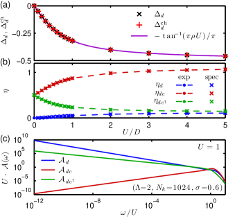
Figure 2: (Color online) Numerical results for the LCM of Eq. (2), for the type 2 quench of Eq. (8), whose initial, final and post-quench initial states $|G_{\rm i}\rangle$, $|G_{\rm f}\rangle$ and $|\psi_{{\rm i}}\rangle$ are depicted in Figs. 1(b,c), 1(d) and 1(e-g), respectively. (a) Comparison of the decay exponent $\Delta_{d}$ obtained from Eq. (31) (crosses) with the displaced charge $\Delta_{d}^{{\rm ch}}$ from Eq. (32) (pluses), for a number of different values of $U$. The two values agree very well (they differ by less than $0.1\%$), also with the analytic prediction Eq. (33) (solid line). As expected, $\Delta_{d}\to-1/2$ for $U\to\infty$. (b) Comparison of two ways of determining the AO exponents $\eta$ that govern the low-energy asymptotic behaviour $\mathcal{A}\sim\omega^{-1+2\eta}$ of the spectral functions of Eqs. (35), related to Figs. 1(e-g): exponents obtained by fitting a power law to the corresponding spectra [shown in (c)] are shown as crosses (marked “spec”, for “spectra”); the corresponding exponents expected from Eq. (35), using the results of (a) for $\Delta_{d}$, are shown as dots (marked “exp” for “expected”). We find a maximal deviation of less than $1\%$. Here and in all similar figures below, the dashed lines are only guides to the eye. (c) Asymptotic low-frequency dependence of the spectra Eqs. (35), for $U=1$, on a double logarithmic plot, allowing the corresponding exponents $\eta$ to be extracted.

In this subsection we present numerical results for the IRLM without tunnelling, corresponding to the local charge model of Eq. (2), depicted in Fig. 1(a). We consider the type 2 quench of Eq. (8), with $\hat{X}^{\dagger}=\hat{d}^{\dagger}$. The initial and final ground states $|G_{\rm i}\rangle$ and $|G_{\rm f}\rangle$ are illustrated in Figs. 1(b,c) and 1(d), respectively, and the post-quench initial state $|\psi_{{\rm i}}\rangle=\hat{d}^{\dagger}|G_{\rm i}\rangle$ in Fig. 1(e). With these choices the overlap $|\langle\psi_{{\rm i}}|G_{\rm f}\rangle|$ of Eq. (11) becomes

$$\mathcal{O}_{d}\equiv|\langle G_{0}|\hat{d}|G_{1}\rangle|=|\langle g_{0}|g_{1}\rangle|\sim N^{-\frac{1}{2}\Delta_{d}^{2}}\,.$$ (31)

The corresponding displaced charge obtained from Eq. (12) is

$$\Delta_{d}^{{\rm ch}}=\langle g_{1}|\hat{n}_{{\rm sea}}|g_{1}\rangle-\langle g_{0}|\hat{n}_{{\rm sea}}|g_{0}\rangle\>,$$ (32)

since $|G_{\rm f}\rangle$ and $|\psi_{{\rm i}}\rangle$ describe the same dot charge, $n_{d}=1$.

We used NRG to calculate the overlap $\mathcal{O}_{d}$ of Eq. (31) and extract the exponent $\Delta_{d}$ from its exponential decay with Wilson chain length [Eq. (30)], for several values of $U$. As consistency check, we also calculated the displaced charge $\Delta_{d}^{{\rm ch}}$ [Eq. (32)]. As shown in Fig. 2(a), the results for $\Delta_{d}$ (crosses) and $\Delta_{d}^{{\rm ch}}$ (pluses) agree very well. The displaced charge $\Delta_{d}^{{\rm ch}}$ is $<0$, since the repulsive interaction pushes charge away from the local site. Its magnitude $|\Delta_{d}^{{\rm ch}}|$ depends on the interaction strength: as $U$ is increased from $0$ to $\infty$, the displaced charge goes from $0$ to $-\frac{1}{2}$, reflecting the complete depletion of the initially half-filled Wilson chain site directly adjacent to the dot site [compare Figs. 1(b) and 1(d)]. Figure 2(a) shows that the numerical results for $\Delta_{d}$ and $\Delta_{d}^{{\rm ch}}$ (symbols) also agree with the analytical result (solid line) obtained for the phase shift obtained from elementary scattering theory [see e.g. Ref. Gogolin, , Eq. (25.29)],

$$\Delta_{d}=-\frac{1}{\pi}\tan^{-1}\left(\pi\rho U\right)\>,$$ (33)

with $\rho$ the density of states in the Fermi sea (cf. Sec. II.5).

To study the influence of AO on dynamical quantities, we consider simple and composite type 2 quenches induced by acting on the initial ground state $|G_{\rm i}\rangle=|G_{0}\rangle$ with the operators

$$\hat{X}^{\dagger}=\hat{d}^{\dagger}\>,\qquad\hat{Y}_{1}^{\dagger}=\hat{c}^{\dagger}\hat{d}^{\dagger}\>,\qquad\hat{Y}_{2}^{\dagger}=\hat{c}\hat{d}^{\dagger}\>.$$ (34)

All three operators describe transitions between the $n_{d}=0$ and $1$ sectors. The analysis of Sec. II.4 applies directly, with the identifications $\hat{H}_{\rm i}=\hat{H}_{0}$ and $\hat{H}_{\rm f}=\hat{H}_{1}$, while $\Delta_{\!\!\;C}=\pm 1$ for $\hat{Y}_{1}^{\dagger}$ or $\hat{Y}_{2}^{\dagger}$, respectively [see Figs. 1(e-g)]. In particular, Eqs. (23) and (25) imply:

$$\mathcal{A}_{d}(\omega) \sim\omega^{-1+2\eta_{d}} \eta_{d} =\tfrac{1}{2}\Delta_{d}^{2}\>,$$ (35a)

$$\mathcal{A}_{dc}(\omega) \sim\omega^{-1+2\eta_{dc}} \eta_{dc} =\tfrac{1}{2}(\Delta_{d}-1)^{2}\>,$$ (35b)

$$\mathcal{A}_{dc^{\dagger}}(\omega) \sim\omega^{-1+2\eta_{dc^{\dagger}}} \eta_{dc^{\dagger}} =\tfrac{1}{2}(\Delta_{d}+1)^{2}\>.$$ (35c)

Using NRG, we calculated these three spectra for several values of $U$ (cf. Fig. 2(c)). In the limit of small $\omega$, the spectra show clear power law behaviour, $\omega^{-1+2\eta}$. The exponents $\eta_{d}$, $\eta_{dc}$, $\eta_{dc^{\dagger}}$ extracted from these spectra are shown in Fig. 2(b) (crosses, marked “spec”, for “spectra”). They agree well with the values expected (dots, marked “exp”, for “expected”) from Eqs. (35), based on the value for $\Delta_{d}$ extracted from Eq. (31). Thus, all ways of determining $\Delta_{d}$ are completely consistent, confirming the validity of the above analysis.

III.2 With tunnelling: IRLM

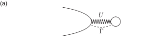
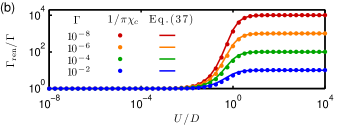
Figure 3: (Color online) (a) Cartoon of the Hamiltonian (III.2) for the IRLM. (b) The renormalized level width $\Gamma_{\rm ren}$, calculated via the dot’s charge susceptibility, $1/\pi\chi_{c}$, Borda2008 (dots) or via Eq. (37) (solid line), shown as a function of $U$ for $\varepsilon_{\!d}=0$ and several values of $\Gamma$. As $U$ increases from 0, $\Gamma_{\rm ren}/\Gamma$ begins to differ significantly from its initial value, namely 1, only once $U$ becomes comparable to the band-width, reaching its maximal value $(\Gamma/D)^{-1/2}$ for $U\gg D$.

The previous subsection focused on a switch between two sectors of the Hilbert space, with $n_{d}=0$ and $n_{d}=1$, that were not coupled dynamically, but governed instead by two distinct Hamiltonians, $\hat{H}_{\rm i}$ and $\hat{H}_{\rm f}$. In the present subsection, we consider the case that the sectors with $n_{d}=0$ and $n_{d}=1$ are coupled by tunnelling between dot and lead, so that the notion of an initial and final Hamiltonian, acting in decoupled sectors of Hilbert space, does not apply. The dynamics is governed instead by the single Hamiltonian $\hat{H}_{\rm i}=\hat{H}_{\rm f}=\hat{H}_{\rm IRLM}$, given by [see Fig. 3(a)]

$$\hat{H}_{\rm IRLM} = \varepsilon_{\!d}\,\hat{d}^{\dagger}\!\hat{d}^{{\phantom{\dagger}}}+U(\hat{d}^{\dagger}\!\hat{d}^{{\phantom{\dagger}}}-1/2)(\hat{c}^{\dagger}\!\hat{c}^{{\phantom{\dagger}}}-1/2)$$

$$+\sum_{\varepsilon}\varepsilon\,\hat{c}_{\varepsilon}^{\dagger}\hat{c}_{\varepsilon}^{{\phantom{\dagger}}}+\sqrt{\frac{\Gamma}{\pi\rho}}\sum_{\varepsilon}(\hat{d}^{\dagger}\!\hat{c}_{\varepsilon}^{{\phantom{\dagger}}}+\hat{c}_{\varepsilon}^{\dagger}\hat{d}^{{\phantom{\dagger}}}\!\!)\>.$$

We assume, here and in all later settings, that the hybridization of the dot level with the Fermi sea states is $\varepsilon$-independent, with $\Gamma$ being the bare width of the dot level. Here, in contrast to the local charge model of Eq. (2), the interaction term is taken to be particle-hole symmetric, so that the model is particle-hole symmetric for $\varepsilon_{\!d}=0$.

The presence of the interaction, $U$, is known to effectively modify the level width,Schlottmann1980 ; Borda2008 both by reducing the density of states of the leads near the dot, and by inducing AO in the leads when the dot occupancy changes. The precise interplay between these effects can be quite intricate and was studied in Ref. Borda2008, . A quantitative analysis can be performed by defining a renormalized level width in terms of the charge susceptibility, $\Gamma_{\rm ren}\equiv 1/\pi\chi_{c}$. At the point of particle-hole (ph) symmetry ($\varepsilon_{\!d}=0$), an analytic formula for the latter is available, Schlottmann1980

$$\Gamma_{\rm ren}/D=(\Gamma/D)^{1/(2-(1+\Delta_{d}^{\rm ph})^{2})}\>,$$ (37)

where $\Delta_{d}^{\rm ph}$ is given by

$$\Delta_{d}^{\rm ph} = -\frac{2}{\pi}\tan^{-1}\left(\pi\rho U/2\right)\>.$$ (38)

$\Delta_{d}^{\rm ph}$ can be interpreted as the change in scattering phase shift that a system with $\Gamma=0$, $\varepsilon_{\!d}=0$ experiences if the local occupancy is changed abruptly from $n_{d}=0$ to $1$. The form of Eq. (38) is analogous to Eq. (33) for $\Delta_{d}$, with two differences: since the final scattering potentials being compared have amplitude $-U/2$ and $U/2$ (instead of $0$ and $U$), the argument of $\tan^{-1}$ has an extra factor of $1/2$, and there is an extra prefactor of $2$.

The dependence of $\Gamma_{\rm ren}$ on $U$ is illustrated in Fig. 3(b), which shows good agreement between the NRG results for $1/\pi\chi_{c}$ (dots) and the analytic formula (37) (lines). For $U$ much smaller than the bandwidth $D$, $\Gamma_{\rm ren}/\Gamma$ is essentially equal to $1$; it strongly increases once $U$ becomes of the order $D$, and saturates to $(\Gamma/D)^{-1/2}$ for $U\gg D$.

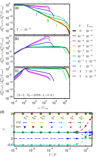
Figure 4: (Color online) (a)-(c) The equilibrium spectral functions $\mathcal{A}^{{\rm eq}}_{d}(\omega)$, $\mathcal{A}^{{\rm eq}}_{dc}(\omega)$ and $\mathcal{A}^{{\rm eq}}_{dc^{\dagger}}(\omega)$ for the IRLM, showing a crossover from trivial power laws, $\omega^{-1+2\eta^{{\rm eq}}}$, for $\omega<\omega^{\ast}$, to AO power laws, $\omega^{-1+2\eta^{0}}$, for $\omega^{\ast}<\omega<D$, with the crossover frequency $\omega^{\ast}$ given by $\Gamma_{\rm ren}$. (d) Comparison of the exponents $\eta^{{\rm eq}}$ (triangles) and $\eta^{0}$ or $\eta_{d}^{\prime}$ (crosses) extracted from the spectra shown in (a-c), with the values expected from Eqs. (39) for $\eta^{\rm eq}$ (solid lines), and from Eqs. (41) for $\eta^{0}$ or from Eq. (40) for $\eta_{d}^{\prime}$ (dashed lines with dots), for several values of $U$. In (a), arrows indicate the scale $\bar{\omega}^{\ast}$ that separates the regimes $\omega^{\ast}<\omega<\bar{\omega}^{\ast}$ and $\bar{\omega}^{\ast}<\omega<D$, where $\mathcal{A}_{d}^{\rm eq}$ scales according to Eqs. (40) or (41a), respectively.

Let us now consider the equilibrium spectral functions for the operators of Eq. (34), $\mathcal{A}^{\rm eq}_{d}$, $\mathcal{A}^{\rm eq}_{dc}$ and $\mathcal{A}^{\rm eq}_{dc^{\dagger}}$. They are defined as in Eq. (22) but with $\hat{H}_{\rm f}=\hat{H}_{\rm i}$, because for the IRLM, where $n_{d}$ is not conserved, none of these operators induces a quench. Therefore, the $\omega\to 0$ behaviour of their correlators is expected (and indeed found) to be independent of AO. However, quite remarkably, traces of AO do show up in an intermediate frequency regime, $\omega^{\ast}<\omega<D$, where $1/\omega^{\ast}$ corresponds to the time scale within which charge equilibration takes place. Below the energy scale $\omega^{\ast}$ the quantum impurity becomes strongly correlated with the Fermi sea and for the present model we have $\omega^{\ast}\simeq\Gamma_{\rm ren}$. Let us therefore discuss the two regimes, $\omega$ below or above $\omega^{\ast}$, separately.

In the regime $\omega\ll\omega^{\ast}$, the spectral functions are found to have the following asymptotic form $\mathcal{A}^{{\rm eq}}\sim\omega^{-1+2\eta^{{\rm eq}}}$ [cf. Figs. 4(a-c)]:

$$\mathcal{A}^{\rm eq}_{d}(\omega) \sim\omega^{0}\>, \eta^{\rm eq}_{d} =1/2\>,$$ (39a)

$$\mathcal{A}^{\rm eq}_{dc}(\omega) \sim\omega^{3}\>, \eta^{\rm eq}_{dc} =2\>,$$ (39b)

$$\mathcal{A}^{\rm eq}_{dc^{\dagger}}(\omega) \sim\omega^{3}\>, \eta^{\rm eq}_{dc^{\dagger}} =2\>.$$ (39c)

The exponents arising here can be understood analytically using elementary, though not entirely trivial arguments, based on the fact that the lowest-lying excitations of this model have Fermi liquid properties. We refer the reader to the Appendix for a detailed analysis.

Now consider the regime $\omega^{\ast}<\omega<D$. As shown in the corresponding regime of $\omega/\Gamma_{\rm ren}>1$ in Figs. 4(a-c), each of the equilibrium spectral functions $\mathcal{A}^{\rm eq}_{d}$, $\mathcal{A}^{\rm eq}_{dc}$ and $\mathcal{A}^{\rm eq}_{dc^{\dagger}}$, exhibits another, different power-law there. For $\mathcal{A}^{\rm eq}_{d}$ we actually find that within this regime two different power-laws can be discerned: First, in a regime $\omega^{\ast}<\omega<\bar{\omega}^{\ast}$ we find,

$$\mathcal{A}_{d}^{{\rm eq}}(\omega) \sim\omega^{-1+2\eta_{d}^{\prime}}\;,\quad\eta_{d}^{\prime}=-\tfrac{1}{2}-\Delta_{d}^{\rm ph}+(\Delta_{d}^{\rm ph})^{2}\;,\qquad\phantom{.}$$ (40)

where $\Delta_{d}^{\rm ph}$ is given by Eq. (38). The exponent $\eta_{d}^{\prime}$ corresponds to the leading correction for weak interactions $(U/D\ll 1)$ to the pure Lorentzian decay of the spectral function of the $d$-level (see Eq. (63) of the Appendix), as can be shown using methods discussed in Refs. Goldstein2009, and Goldstein2010b, . The scale $\bar{\omega}^{\ast}$ that sets the upper limit for this behaviour is marked by arrows in Fig. 4(a) and decreases with increasing $U/D$. For $U/D$ sufficiently small that $\bar{\omega}^{\ast}$ lies far below the bandwidth $D$, we find a second power law within the window $\bar{\omega}^{\ast}<\omega<D$, namely

$$\mathcal{A}^{\rm eq}_{d}(\omega) \sim\omega^{-1+2\eta_{d}^{0}}, \eta_{d}^{0} =\tfrac{1}{2}(\Delta_{d}^{\rm ph})^{2}\>.$$ (41a)

For the other two spectral functions we find throughout the regime $$\omega^{\ast}<\omega<D$$:

$$\mathcal{A}^{\rm eq}_{dc}(\omega) \sim\omega^{-1+2\eta_{dc}^{0}}, \eta_{dc}^{0} =\tfrac{1}{2}(\Delta_{d}^{\rm ph}-1)^{2}\>,$$ (41b)

$$\mathcal{A}^{\rm eq}_{dc^{\dagger}}(\omega) \sim\omega^{-1+2\eta^{0}_{dc^{\dagger}}}, \eta^{0}_{dc^{\dagger}} =\tfrac{1}{2}(\Delta_{d}^{\rm ph}+1)^{2}\>.$$ (41c)

Remarkably, Eqs. (41) have the same form as Eqs. (35), except that $\Delta_{d}$ is replaced by $\Delta_{d}^{\rm ph}$ of Eq. (38), i.e. by the AO exponent involved in abruptly changing the local occupancy from $0$ to $1$ (in the absence of tunnelling). That this exponent should emerge is natural, since the corresponding correlators $\mathcal{G}_{d}$, $\mathcal{G}_{dc}$ and $\mathcal{G}_{dc^{\dagger}}$ all involve an operator $d^{\dagger}$ that places an electron on the dot at time $t=0$. Although the dot occupancy $n_{d}(t)$ will relax back to its initial value $n_{d}^{{\rm i}}$ in the long time limit, this requires times $t\gg 1/\omega^{\ast}$. In contrast, the lead electrons react to the change in local charge on the much shorter time scale $1/D$. Thus, in the window of intermediate times, $1/D\ll t\ll 1/\omega^{\ast}$, corresponding to frequencies $\omega^{\ast}\ll\omega\ll D$, the situation is similar to that of the previous subsection, where we had $\Gamma=0$ and a change in dot occupancy from $0$ to $1$ induced changes in the lead phase shifts, accompanied by AO. Thus, the exponents $\eta^{0}$ arising in Eq. (41) can be identified as the (equilibrium) scaling dimensions of the corresponding operators calculated in the absence of tunnelling (which is why we use a superscript $0$ on such exponents, here and below). This explains the similarity between the behaviour described by Eqs. (41) and Eqs. (35). Note that the scaling dimension $\eta^{0}_{dc^{\dagger}}$ [Eq. (41c)] of the tunnelling operators $\hat{d}\hat{c}^{\dagger}$ and $\hat{c}^{\dagger}\!\hat{d}$ satisfy $0\leq\eta^{0}_{dc^{\dagger}}\leq 1/2$ [since for $U>0$, we have $-1\leq\Delta_{d}^{\rm ph}\leq 0$, by Eq. (38)], thus tunnelling is always relevant for this model.

We conclude this subsection with a comment on the fact that $\mathcal{A}^{\rm eq}_{d}(\omega)$ crosses over from non-AO behaviour [Eq. (40)] to AO behaviour [Eq. (41a)] as $U/D$ is increased past 1. AO behaviour is absent for $U/D\ll 1$ because this situation corresponds essentially to a non-interacting resonant-level model, for which $\mathcal{G}_{d}^{\rm eq}(t)$ does not show power-law behaviour of the type assumed in Eq. (18); instead it decays exponentially ($\sim e^{-\Gamma t}$), causing the spectral function $\mathcal{A}^{\rm eq}_{d}(\omega)$ to have an essentially Lorentzian form. Equation (40) is the large-frequency limit of the latter, but including the leading corrections in $U/D$, calculated using methods discussed in Refs. Goldstein2009, and Goldstein2010b, . However, once $U/D$ becomes $\gtrsim 1$, AO does begin to matter, implying a regime of power-law decay for $\mathcal{G}_{d}^{\rm eq}(t)$ on intermediate time scales, leading to Eq. (41a) for $\mathcal{A}^{{\rm eq}}_{d}(\omega)$.

III.3 Quantum quench of level position

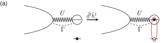
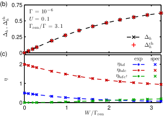
Figure 5: (Color online) (a) Cartoon of the quench which occurs when an electron-hole pair is created at time $t=0$, see Eq. (43). (The cartoon depicts the situation relevant for exciton creation by absorption of a photon, which excited an electron from a valence-band to a conduction band level of a semiconducting quantum dot.) (b) The exponent $\Delta_{\!\!\;h}$ [from Eq. (11)] and the displaced charge $\Delta_{\!\!\;h}^{{\rm ch}}$ [from Eq. (12)], for the quench of Eq. (42), as function of the quench range $W$. (c) Corresponding values of the AO exponents $\eta_{hd}$, $\eta_{hdc}$ and $\eta_{hdc^{\dagger}}$, extracted from the asymptotic behaviour $\omega^{-1+2\eta}$ of spectral functions (crosses), or as expected from Eqs. (46) (dots). Typically, relative errors are less than $1\%$.

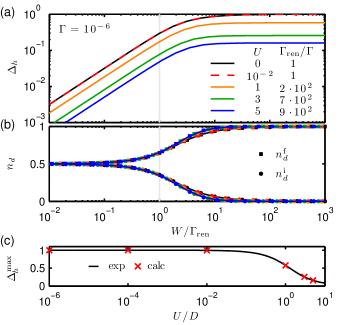
Figure 6: (Color online) (a) The AO exponent $\Delta_{\!\!\;h}$ [extracted according to Eq. (11)] as function of $W/\Gamma_{\rm ren}$, for several values of $U$. For $W/\Gamma_{\rm ren}\gg 1$, $\Delta_{\!\!\;h}$ approaches its maximal value $\Delta_{\!\!\;h}^{\rm max}$. As $W$ is reduced below $\Gamma_{\rm ren}$, $\Delta_{\!\!\;h}$ drops below its maximal value and decreases with $W$ [linearly so for $W/\Gamma_{\rm ren}\ll 1$]. (b) The final and initial occupancies $n_{d}^{\rm f}$ (squares, upper curves) and $n_{d}^{\rm i}$ (circles, lower curves) as functions of $W/\Gamma_{\rm ren}$, for the same values of $U$ [same color code as in (a)]. (c) The maximal value $\Delta_{\!\!\;h}^{\rm max}$ of the AO exponent $\Delta_{\!\!\;h}$, extracted from the $W/\Gamma_{\rm ren}\gg 1$ regime of (a) (crosses, “calc”), or expected from Eq. (44) (solid line, “exp”); the relative deviations are well below $1\%$.

In the previous subsection we emphasized the importance of the scale $\omega^{\ast}$, which separates the low- and intermediate-frequency regimes, showing trivial exponents or AO exponents, respectively. It is instructive to study the role of the scale $\omega^{\ast}$ in a slightly different but related context, namely quench spectral functions involving a quantum quench of the level position. This will shed further light on the AO between states with different local level occupancies.

Concretely, we consider initial and final Hamiltonians that both are of the form Eq. (III.2), but with initial and final level positions that are symmetrically spaced on opposite sides of the model’s symmetry point at $\varepsilon_{\!d}=0$:

$$\varepsilon_{\!d}^{{\rm i}}=W/2\quad\stackrel{{\scriptstyle{\rm quench}}}{{\longrightarrow}}\quad\varepsilon_{\!d}^{{\rm f}}=-W/2\>.$$ (42)

Although this is an example of a type 1 quench, it will be convenient (mainly for notational reasons) to reformulate this situation as a type 2 quench. To this end we use the Hamiltonian

$$\hat{H} = W(1/2-\hat{n}_{h})\hat{n}_{d}+U(\hat{n}_{d}-1/2)(\hat{c}^{\dagger}\!\hat{c}-1/2)\qquad\phantom{.}$$ (43)

$$+\sum_{\varepsilon}\varepsilon\,\hat{c}_{\varepsilon}^{\dagger}\hat{c}_{\varepsilon}^{{\phantom{\dagger}}}+\sqrt{\frac{\Gamma}{\pi\rho}}\sum_{\varepsilon}(\hat{d}^{\dagger}\!\hat{c}_{\varepsilon}^{{\phantom{\dagger}}}+\hat{c}_{\varepsilon}^{\dagger}\hat{d})\>,$$

where we have introduced an auxiliary degree of freedom, called “hole” (in analogy to the role of holes in exciton creation by optical absorptionHelmes2005 ; Tureci2011 ; Latta2011 ), with hole counting operator $\hat{n}_{h}=\hat{h}^{\dagger}\hat{h}$. The hole has no dynamics; its only role is to distinguish two distinct sectors of Hilbert space, in which the dynamics is described by $\hat{H}_{\rm i}$ or $\hat{H}_{\rm f}$, with hole number $n_{h}=0$ or $1$, respectively [see Fig. 5(a)]. The type 2 quench that switches between these sectors is induced by $\hat{X}^{\dagger}=\hat{h}^{\dagger}$. The overlap $\mathcal{O}_{h}\sim N^{-\frac{1}{2}\Delta_{\!\!\;h}^{2}}$ between the initial and final ground states is characterized by an AO exponent $\Delta_{\!\!\;h}$ [Eq. (11)] that is equal to the charge $\Delta_{\!\!\;h}^{{\rm ch}}$ displaced by the quench [Eq. (12)].

The magnitude of $\Delta_{\!\!\;h}$ increases with the range $W$ of the quench, as shown in Fig. 5(b) (linear scale) and Fig. 6(a) (log-log scale). Note, in particular, that the scale on which the quenching range, $W$, needs to change in order for the AO exponents to change significantly, is given by $\Gamma_{\rm ren}$. This is natural: when $W\gg\Gamma_{\rm ren}$, the two states $|G_{\rm i}\rangle$ and $|G_{\rm f}\rangle$ connected by the quench describe dots with strongly different occupancies, $n_{d}^{{\rm i}}\simeq 0$ vs. $n_{d}^{{\rm f}}\simeq 1$, see Fig. 6(b). Hence the AO [Eq. (11)] of the corresponding Fermi seas will be strong. The maximum possible value of the exponent $\Delta_{\!\!\;h}$ is

$$\Delta_{\!\!\;h}^{\rm max}=1+\Delta_{d}^{\rm ph}\>,$$ (44)

with $\Delta_{d}^{\rm ph}(U)<0$ given by Eq. (38). The first term simply gives the $U\to\infty$ value of the change in dot occupancy induced by the quench, namely $1$; the second term reflects the reaction of the Fermi sea to this change, cf. Sec. III.2.

Following the arguments of Sec. II.4, the nonequilibrium spectral functions $\mathcal{A}_{Y}(\omega)$, defined for

$$\hat{Y}_{1}^{\dagger}=\hat{d}^{\dagger}\hat{h}^{\dagger}\>,\qquad\hat{Y}_{2}^{\dagger}=\hat{c}^{\dagger}\hat{d}^{\dagger}\hat{h}^{\dagger}\>,\qquad\hat{Y}_{3}^{\dagger}=\hat{c}\,\hat{d}^{\dagger}\hat{h}^{\dagger}\>,$$ (45)

are expected to show the following AO behaviour for ${\omega\to 0}$:

$$\mathcal{A}_{hd}(\omega) \sim\omega^{-1+2\eta_{hd}} \eta_{hd} =\tfrac{1}{2}(\Delta_{\!\!\;h}-1)^{2}\>,$$ (46a)

$$\mathcal{A}_{hdc}(\omega) \sim\omega^{-1+2\eta_{hdc}} \eta_{hdc} =\tfrac{1}{2}(\Delta_{\!\!\;h}-2)^{2}\>,$$ (46b)

$$\mathcal{A}_{hdc^{\dagger}}(\omega) \sim\omega^{-1+2\eta_{hdc^{\dagger}}} \eta_{hdc^{\dagger}} =\tfrac{1}{2}\Delta_{\!\!\;h}^{2}\>.$$ (46c)

The reason for the specific form of the exponents is that for the correlators $\mathcal{G}_{hd}$, $G_{hdc}$ or $G_{hdc^{\dagger}}$, at $t=0$ the local charge (on the d-level or in the Fermi sea) is increased by one, two or zero, respectively [i.e. $\Delta_{\!\!\;C}=1$, $2$ or $0$ in Eq. (16)]. Figure 5(c) shows that the exponents (crosses) extracted from the asymptotic behaviour $\mathcal{A}_{Y}(\omega)$ are indeed in good agreement with values expected (dots) from Eqs. (46).

IV Population Switching without Sensor

The models investigated so far served as testing ground for the influence of AO on various types of spectral functions. The following two sections have the concrete motivation to clarify the role of AO in the context of quantum dot models that display the phenomenon of population switching (PS). Hackenbroich1997 ; Baltin1999 ; Silvestrov2000 ; Silvestrov2001 ; Golosov2006 ; Karrasch2007 ; Goldstein2010 ; Goldstein2011 In such models, a quantum dot, tunnel-coupled to leads, contains levels of different widths and is capacitively coupled to a gate voltage that shifts the levels energy relative to the Fermi level of the leads. Under suitable conditions, an (adiabatic) sweep of the gate voltage induces an inversion in the population of these levels (a so-called population switch), implying a change in the local potential seen by the Fermi seas in the leads. Goldstein, Berkovits and Gefen (GBG) have argued in Ref. Goldstein2010, ; Goldstein2011, that in this context AO can play an important role. In particular, they pointed out that for a model involving a third lead acting as a charge sensor, the effects of AO can be enhanced to such an extent that population switching becomes abrupt, i.e. turns into a phase transition. Our goal is to elucidate the influence of AO by using the tools developed above in the context of the IRLM.

In the present section, we will study population switching in a two-lead model (without charge sensor), which is equivalent to an anisotropic Kondo model. Goldstein2010 ; Goldstein2011 ; Kashcheyevs2007 ; Lee2007 ; Silvestrov2007 ; Kashcheyevs2009 The corresponding Kondo temperature, $T_{\rm K}$, sets the width of the population switch as function of gate voltage. We calculate the spectral function $\mathcal{A}_{Y}^{\rm eq}(\omega)$ of the pseudospin-flip operator and show that $T_{\rm K}$ also acts as the crossover scale $\omega^{\ast}$ that separates a low-frequency regime showing Fermi-liquid power laws from an intermediate-frequency regime revealing AO exponents. We investigate the origin of the latter by a quantum quench analysis similar to that of Sec. III.3 above. In the following section, we will generalize the model by adding a charge sensor and analyse how this enhances the effects of AO.

IV.1 Width of switching regime

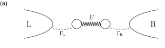
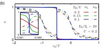
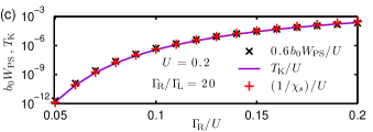
Figure 7: (Color online) (a) Cartoon of the Hamiltonian (IV.1) for the asymmetric SIAM. (b) The occupations $n_{\rm L}$ (solid lines) and $n_{\rm R}$ (dashed lines) of the left and right level, respectively, as functions of $\varepsilon_{\!d}$, for several values of $\Gamma_{\!\rm R}$, at a fixed ratio of $\Gamma_{\!\rm R}/\Gamma_{\!\rm L}=20$. As $\varepsilon_{\!d}$ is lowered past the particle-hole symmetric point at $\varepsilon_{\!d}=-U/2$, population switching occurs, with $n_{R}$ changing from near $1$ to near $0$, and vice versa for $n_{\rm L}$. Inset: zoom into the switching region around $\varepsilon_{\!d}=-U/2$, showing that the switch is continuous (as function of $\varepsilon_{\!d}$) even though the switching region becomes narrower for decreasing $\Gamma_{\!\rm R}$. (c) Comparison of $b_{0}W_{\rm PS}$ [from Eqs. (48) and (51), crosses], $T_{\rm K}$ [from Eq. (52), solid], and the inverse pseudospin susceptibility $1/\chi_{s}$ (pluses). All three quantities evidently decrease similarly with decreasing $\Gamma_{R}/U$.

We consider a model involving two single-level dots (${\mu={\rm L,R}}$) and for convenience choose their level energies $\varepsilon_{\!d}$ to be equal, so that the PS always occurs at the particle-hole symmetric point, $\varepsilon_{\!d}=-U/2$. (Note that PS occurs also for nondegenerate levels, as long as their level spacing is smaller than the difference of their level widths $\Gamma_{\!\!\mu}$.) The levels have an electrostatic coupling $U>0$ and are each tunnel-coupled to its own lead [see Fig. 7(a)]:

$$\hat{H}_{\rm SIAM} = \sum_{\mu}\varepsilon_{\!d}\,\hat{d}_{\mu}^{\dagger}\hat{d}_{\mu}^{{\phantom{\dagger}}}+U\hat{d}_{\rm L}^{\dagger}\hat{d}_{\rm L}^{{\phantom{\dagger}}}\hat{d}_{\rm R}^{\dagger}\hat{d}_{\rm R}^{{\phantom{\dagger}}}$$

$$+ \sum_{\varepsilon\mu}\varepsilon\,\hat{c}_{\varepsilon\mu}^{\dagger}\hat{c}_{\varepsilon\mu}^{{\phantom{\dagger}}}+\sum_{\mu}\sqrt{\frac{\Gamma_{\!\!\mu}}{\pi\rho}}\sum_{\varepsilon}(\hat{d}_{\mu}^{\dagger}\hat{c}_{\varepsilon\mu}^{{\phantom{\dagger}}}+\hat{c}_{\varepsilon\mu}^{\dagger}\hat{d}_{\mu}^{{\phantom{\dagger}}})\>,$$

(We use notation analogous to that of Sec. III.2.) We choose the level widths to be strongly asymmetric and will use a fixed value of their ratio, $\Gamma_{\!\rm R}/\Gamma_{\!\rm L}=20$, throughout. The model thus has the form of a spin-asymmetric single-impurity Anderson model (SIAM), where $\mu$ acts as pseudospin index.

As illustrated in Fig. 7(b), this model shows PS when $\varepsilon_{\!d}$ is decreased past $\varepsilon_{\!d}=-U/2$ (the particle-hole symmetric point): as this “switching point” is crossed, the occupancy of the broad level (dashed lines) changes from near $1$ to near $0$, and vice versa for the narrow level (solid lines). We define the width of the switching regime, $W_{\rm PS}$, as the difference,

$$W_{\rm PS}\equiv\varepsilon_{\!d}(n_{\rm R+})-\varepsilon_{\!d}(n_{\rm R-})\>,$$ (48)

between those two values of $\varepsilon_{\!d}$, located symmetrically on either side of the switching point, at which the occupation of the right level is $n_{\rm R+}\equiv\tfrac{3}{4}n_{\rm R+}^{\rm max}$ $(>\tfrac{1}{2})$ or $n_{\rm R-}=1-n_{\rm R+}$ ($<\tfrac{1}{2})$, respectively, where $n_{\rm R+}^{\rm max}$ is the largest value reached by $n_{\rm R}$ for $\varepsilon_{\!d}>-U/2$, to the right of the PS.

Figure 7(b) and its inset show that the width of the switching regime decreases with decreasing $\Gamma_{\!\!\mu}$, without, however, dropping to zero as long as the level widths are nonzero. This behaviour can be understood as follows. Goldstein2010 ; Goldstein2011 ; Kashcheyevs2007 ; Lee2007 ; Silvestrov2007 ; Kashcheyevs2009 In the vicinity of the particle-hole symmetric point, only two local charge configurations are relevant, namely those with occupancies $(n_{\rm L},n_{\rm R})$ equal to $(0,1)$ or $(1,0)$. The spin-asymmetric SIAM can thus be mapped onto an anisotropic Kondo model by a Schrieffer-Wolff transformation. This leads to an anisotropic pseudospin exchange interaction of the form

$$\hat{H}_{\rm exch} = (U_{\rm L}+U_{\rm R})(\hat{d}_{\rm L}^{\dagger}\hat{d}_{\rm L}^{{\phantom{\dagger}}}-\hat{d}_{\rm R}^{\dagger}\hat{d}_{\rm R}^{{\phantom{\dagger}}})(\hat{c}_{\rm L}^{\dagger}\hat{c}_{\rm L}^{{\phantom{\dagger}}}-\hat{c}_{\rm R}^{\dagger}\hat{c}_{\rm R}^{{\phantom{\dagger}}})$$ (49)

$$+2\sqrt{U_{\rm L}U_{\rm R}}(\hat{c}_{\rm L}^{{\phantom{\dagger}}}\hat{c}_{\rm R}^{\dagger}\hat{d}_{\rm L}^{\dagger}\hat{d}_{\rm R}^{{\phantom{\dagger}}}+{\rm h.c.})$$

$$+B_{\rm eff}(\hat{d}_{\rm L}^{\dagger}\hat{d}_{\rm L}^{{\phantom{\dagger}}}-\hat{d}_{\rm R}^{\dagger}\hat{d}_{\rm R}^{{\phantom{\dagger}}})/2\>,$$

respectively, with coupling constants given by

$$\rho U_{\!\mu}=\frac{\Gamma_{\!\!\mu}}{\pi}\left(\frac{1}{\varepsilon_{\!d}+U}+\frac{1}{|\varepsilon_{\!d}|}\right)\>,$$ (50)

and effective magnetic field

$$B_{\rm eff}=b_{0}(\varepsilon_{\!d}+U/2),\quad b_{0}=\frac{4(\Gamma_{\!\rm R}-\Gamma_{\!\rm L})}{\pi U}\>.$$ (51)

The corresponding Kondo temperature is given by the following expression: Kashcheyevs2007

$$T_{\rm K}=\frac{\sqrt{U(\Gamma_{\!\rm L}+\Gamma_{\!\rm R})}}{\pi}\exp\left[\frac{\pi\varepsilon_{\!d}(U+\varepsilon_{\!d})}{2U(\Gamma_{\!\rm L}-\Gamma_{\!\rm R})}\ln\frac{\Gamma_{\!\rm L}}{\Gamma_{\!\rm R}}\right]\>.$$ (52)

Note that $T_{\rm K}$ decreases exponentially if $\Gamma_{\!\!\mu}$ is decreased with a fixed ratio of $\Gamma_{\!\rm R}/\Gamma_{\!\rm L}$ and actually becomes zero for $\Gamma_{\!\!\mu}=0$ (the argument of the exponent in Eq. (52) is negative, since $\varepsilon_{\!d}<0$).

Now, $T_{\rm K}$ can be associated with the energy gained by forming a ground state involving a screened local pseudospin, which in the present setting translates to a ground state involving a coherent superposition of configurations with local occupancies $(0,1)$ and $(1,0)$. Screening will cease when $\varepsilon_{\!d}$ deviates sufficiently from the symmetry point $-U/2$ that the effective magnetic field $|B_{\rm eff}|$ exceeds $T_{\rm K}$, in which case the ground state will be dominated solely by the $(0,1)$ or $(1,0)$ configuration, instead of involving a coherent superposition of both. Thus the switching width will be set by $b_{0}W_{\rm PS}\simeq T_{\rm K}$, up to a numerical constant of order unity.

Figure 7(c) confirms this expectation. It shows that $b_{0}$ times the switching width $W_{\rm PS}$ [from Eq. (48)] (crosses) and the Kondo temperature $T_{\rm K}$ at $\varepsilon_{\!d}=-U/2$ [from Eq. (52)] (solid line), when plotted as functions of $\Gamma_{\!\rm R}/U$ at fixed $\Gamma_{\!\rm R}/\Gamma_{\!\rm L}$, are indeed almost perfectly proportional to each other. As a numerical consistency check, Fig. 7(c) also shows the inverse of the zero-temperature pseudospin susceptibility of the dot levels, $1/\chi_{s}$ (pluses), confirming that $T_{\rm K}=1/\chi_{s}$. (This is analogous to the relation $\Gamma_{\rm ren}=1/\pi\chi_{c}$ of Sec. III.2.)

IV.2 AO in dynamics of pseudospin-flip operator

Figure 8: (Color online) (a) The pseudospin-flip spectral function $\mathcal{A}^{{\rm eq}}_{Y}(\omega)$ [cf. Eq. (53)] for the PS model without charge sensor, for several values of $\Gamma_{\!\rm R}/U$ with fixed ratio $\Gamma_{\!\rm R}/\Gamma_{\!\rm L}$, calculated at $\varepsilon_{\!d}=-U/2$: plotting $\mathcal{A}^{\rm eq}_{Y}(\omega)/\mathcal{A}^{\rm eq}_{Y}(T_{\rm K})$ versus $\omega/T_{\rm K}$ yields a scaling collapse. The frequency dependence of the curves qualitatively changes at $T_{\rm K}$: for $\omega<T_{\rm K}$ we find Fermi liquid behaviour, $\sim\omega^{3}$ (dotted line), while for $\omega>T_{\rm K}$ each curve shows a nontrivial AO power-law, $\sim\omega^{-1+2\eta_{Y}^{0}}$ [Eq. (54)], exemplified by the dashed and dash-dotted lines for $\Gamma_{\!\rm R}/U=0.2$ and $0.05$, respectively. (b) Comparison of the values for $\eta_{Y}^{0}$ expected from Eq. (54b) (solid line), or extracted from the spectral function $\mathcal{A}_{Y}^{\rm eq}(\omega)$ by using Eq. (54a) in the intermediate-frequency regime between $T_{\rm K}$ and the high frequency maximum (crosses). The accuracy of this extraction deteriorates with increasing $\Gamma_{\!\rm R}/U$, since this reduces the width of the latter regime [see (a)], causing the relative error between crosses and solid line to increases from $1\%$ for $\Gamma_{\!\rm R}/U=0.05$ to $10\%$ for $\Gamma_{\!\rm R}/U=0.2$.

Let us now explore the role of AO in population switching. To this end, we note that the effective exchange interaction $\hat{H}_{\rm exch}$ of Eq. (49) is similar in structure to the IRLM of Eq. (III.2): both involve two charge configurations (the former (0,1) and (1,0), the latter 0 and 1), which induce different phase shifts in the leads due to a dot-lead interaction term, and which are connected by a tunnelling term. More formally, the relation between the IRLM and PS is revealed by the equivalence of both models to the Kondo model (for the IRLM, this equivalence is discussed, e.g., in Refs. Gogolin, ; Schlottmann1980, ; Borda2008, ). Thus, we may expect AO to play a similar role for both models, and hence perform an analysis similar to that in Sections III.2 and III.3.

Specifically, let us study the spectral function $\mathcal{A}^{{\rm eq}}_{Y}(\omega)$ of the pseudospin-flip operators occurring in $\hat{H}_{\rm exch}$,

$$\hat{Y}^{\dagger}=\hat{c}_{\rm L}^{{\phantom{\dagger}}}\hat{c}_{\rm R}^{\dagger}\hat{d}_{\rm L}^{\dagger}\hat{d}_{\rm R}^{{\phantom{\dagger}}}\>,\qquad\hat{Y}=\hat{d}_{\rm R}^{\dagger}\hat{d}_{\rm L}^{{\phantom{\dagger}}}\hat{c}_{\rm R}^{{\phantom{\dagger}}}\hat{c}_{\rm L}^{\dagger}\>.$$ (53)

These induce transitions between the local charge configurations (0,1) and (1,0) and simultaneously add an electron to one lead while removing an electron from the other. (Such a transition does not constitute a quench, since for the present model $n_{d}$ is not conserved.) $\mathcal{A}^{{\rm eq}}_{Y}$ should, in some respects, be analogous to $\mathcal{A}_{dc^{\dagger}}$ of Sec. III.2. We have thus calculated $\mathcal{A}^{{\rm eq}}_{Y}$ numerically, using the Hamiltonian $\hat{H}_{\rm SIAM}$ of Eq. (IV.1). Indeed, Fig. 8(a), which shows $\mathcal{A}^{\rm eq}_{Y}(\omega)$ for several values of $\Gamma_{\!\rm R}/U$, exhibits several features reminiscent of Fig. 4(c) for $\mathcal{A}_{dc^{\dagger}}(\omega)$: (i) A crossover scale $\omega^{\ast}$, separating a regime of very low frequencies from one of intermediate frequencies, is clearly discernible; it is given by $\omega^{\ast}\simeq T_{\rm K}$. (ii) When properly rescaled by plotting $\mathcal{A}^{\rm eq}_{Y}(\omega)/\mathcal{A}^{\rm eq}_{Y}(\omega^{\ast})$ versus $\omega/\omega^{\ast}$, all curves collapse onto each other in the regime $\omega\lesssim D$. (iii) In the low-frequency regime $\omega\ll\omega^{\ast}$ we find the same Fermi-liquid power law, $\mathcal{A}^{\rm eq}_{Y}(\omega)\sim\omega^{3}$ (dotted line), as for $\mathcal{A}_{dc^{\dagger}}(\omega)$ [cf. Eq. (39c)]. (An analytical explanation for this fact is given in at the end of the Appendix.) (iv) In an intermediate-frequency regime $\omega^{\ast}\lesssim\omega\lesssim\omega_{\rm he}$, whose upper limit $\omega_{\rm he}$ is a high-energy scale set by the minimum of the bandwidth or the cost of local charge fluctuations, we find an AO-dominated power law,

$$\mathcal{A}^{\rm eq}_{Y}(\omega) \sim \omega^{-1+2\eta_{Y}^{0}},\quad\omega^{\ast}\lesssim\omega\lesssim\omega_{\rm he}\>.$$ (54a)

Though the numerical calculation of $$\mathcal{A}^{\rm eq}_{Y}(\omega) \hat{H}_{\rm SIAM} \omega>\omega^{\ast} \eta_{Y}^{0} \omega\to 0 \hat{H}_{\rm exch}$$ was performed using the full Hamiltonian of Eq. (IV.1), tunnelling is not important on the short time-scales that govern the frequency regime . Hence, we expect the exponent found from Eq. (54a) to be equal in value to that which one would obtain in the limit of a calculation performed in the absence of pseudospin-flips, i.e. using without the pseudospin-flip terms in the second line of Eq. (49) (but retaining its first and third lines).

Without pseudospin-flips, the correlator involving $\hat{Y}$ would actually constitute a type 2 quench correlator, because $\hat{Y}^{\dagger}$ changes $(\hat{n}_{\rm L}-\hat{n}_{\rm R})$, which is a conserved quantum number for Hamiltonians without pseudospin-flips. Therefore, the expected value of $\eta_{Y}^{0}$ can be predicted using the generalized Hopfield rule [Eq. (25)]. For the present case of two channels that are not interconnected by tunnelling, so that the total charge within each channel is conserved, it can be applied to each channel separately, adding the corresponding exponents Weichselbaum2011 [cf. Eq. (27)]:

$$\eta_{Y}^{0}=\tfrac{1}{2}(\Delta_{\rm L}+1)^{2}+\tfrac{1}{2}(-\Delta_{\rm R}-1)^{2}\>.$$ (54b)

Here $\Delta_{\mu}$ describes the change in phase shift, divided by $\pi$, induced in lead $\mu$ by a pseudospin-flip; it is given by Eq. (38), with $U$ replaced by $U_{\!\mu}$ [from Eq. (50)]. The applicability of these arguments is confirmed by Fig. 8(b), which shows that the exponents extracted from the numerical spectra (crosses) agree quite well with the values expected from Eq. (54b) (solid line). The quality of the agreement deteriorates with increasing $\Gamma_{\!\rm R}/U$, because this reduces the width of the intermediate-frequency regime, making an accurate extraction of $\eta_{Y}^{0}$ from $\mathcal{A}_{Y}^{\rm eq}(\omega)$ increasingly difficult.

Equation (54b) allows us to understand why PS is always continuous in this model: Since $-1\leq\Delta_{\mu}\leq 0$, the scaling dimension of $\hat{Y}$ satisfies $\eta_{Y}\leq 1$, implying that this operator always remains a relevant perturbation that does not flow to zero at low energy scales. This means that AO, although present, is not strong enough to completely suppress the amplitude for pseudospin-flip transitions. Hence, the two sectors (0,1) and (1,0) are always coupled by the effective low-energy Hamiltonian, so that population switching is continuous.Goldstein2010 ; Goldstein2011

IV.3 AO induced by quench of level positions

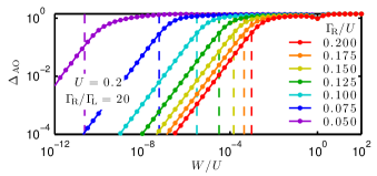
Figure 9: (Color online) AO for the PS model without charge sensing. The exponent $\Delta_{\rm AO}$ [extracted from Eq. (1)] (solid lines with dots) is shown as function of quench size $W/U$ [Eq. (55)], for several values of $\Gamma_{\!\rm R}/U$ with fixed ratio $\Gamma_{\!\rm R}/\Gamma_{\!\rm L}$, showing that AO becomes significant once $W$ increases past $T_{\rm K}/b_{0}$ (indicated by dashed vertical lines). The exponent $\Delta_{\rm AO}$ increases linearly with $W$ for $W\ll T_{\rm K}/b_{0}$, and saturates to a maximal value of $\sqrt{2}$ [Eq. (56)] for $W\gg T_{\rm K}/b_{0}$. The corresponding values of $\Delta_{\rm ch}$ [from Eq. (7)] are not shown but agree with $\Delta_{\rm AO}$ with relative errors of a few percent.

As mentioned above, the operators $\hat{Y}^{\dagger}$ and $\hat{Y}$ connect two configurations with different local occupancies, (0,1) and (1,0). To shed further light on the AO between such configurations, we now perform a quantum quench analysis similar to that of Sec. III.3. We consider a type 1 quench, $\hat{H}_{\rm i}\to\hat{H}_{\rm f}$, induced by changing the level position $\varepsilon_{\!d}$ from a value above the symmetry point, favouring (0,1), to one below, favouring (1,0):

$$\varepsilon_{\!d}^{{\rm i}}=-U/2+W/2\quad\stackrel{{\scriptstyle{\rm quench}}}{{\longrightarrow}}\quad\varepsilon_{\!d}^{{\rm f}}=-U/2-W/2\>.$$ (55)

The corresponding ground states, $|G_{{\rm i}}\rangle$ and $|G_{\rm f}\rangle$, will display AO as in Eq. (1). Based on the lessons learnt from Sec. III.3, the corresponding exponent $\Delta_{\rm AO}$ will increase with the width $W$ of the quench. Indeed, Fig. 9 [to be compared with Fig. 6(a)] shows that $\Delta_{\rm AO}$ increases from close to $0$ for $W$ much below $T_{\rm K}/b_{0}$ (indicated by vertical dashed lines) to a maximal value of

$$\Delta_{\rm AO}^{\rm max}=\sqrt{(1)^{2}+(1)^{2}}=\sqrt{2}$$ (56)

for $W\gg T_{\rm K}/b_{0}$. This maximal value reflects the displaced charge $\Delta_{\rm ch}$ [cf. Eq. (7)] induced by a very strong quench: both $n_{\rm L}$ and $n_{\rm R}$ are $\simeq 0$ (or $\simeq 1$) if the level position is far above (or below) the Fermi energy, $\varepsilon_{\!d}^{{\rm i}}=-U/2+W/2\gg 0$ (or $\ll 0$), cf. Fig. 7(b), thus the displaced charge associated with both $n_{\rm L}$ and $n_{\rm R}$ is $1$. (The contribution to $\Delta_{\rm ch}$ from the leads turns out to be negligible here, Weichselbaum2011 since for sufficiently large $W$ the Fermi sea is essentially decoupled from the dot.)

IV.4 Summary for PS without sensor

The results of this section can be summarized as follows: (i) The energy scale setting the width of PS is proportional to $T_{\rm K}$. (ii) This can directly be attributed to AO: as shown in Fig. 9, the ground states of two configurations on opposite sides of the switching points exhibit strong AO when their level positions differ by more than $T_{\rm K}/b_{0}$. Thus, quantum fluctuations between them, induced by operators such as $\hat{Y}$ and $\hat{Y}^{\dagger}$, are strongly suppressed. (iii) For the present model PS will always be continuous as a function of $\varepsilon_{\!d}$, because (for given $U$) $T_{\rm K}$ is nonzero for any fixed choice of $\Gamma_{\!\rm L}$ and $\Gamma_{\!\rm R}$ (although exponentially small), and AO ceases to be important ($\Delta_{\rm AO}\simeq 0$) once $\varepsilon_{\!d}$ comes within $T_{\rm K}/b_{0}$ of the switching point. Conversely, however, it should now also be plausible that an essentially abrupt PS will be achievable if, by a suitable modification of the model, the degree of AO between the configurations (0,1) and (1,0) can be enhanced sufficiently to push $T_{\rm K}$ to zero even for finite $\Gamma_{\!\rm L}$ and $\Gamma_{\!\rm R}$. As pointed out by GBG, Goldstein2010 ; Goldstein2011 this can be achieved by adding a charge sensor, to which we turn next.

V Population Switching with Sensor

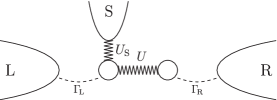
Figure 10: Cartoon of the Hamiltonian (V.1), describing an asymmetric SIAM with an additional sensor lead coupled electrostatically to the left dot.

In this section we study the effects of adding an electrostatically coupled charge sensor to the model of the previous section, as proposed by GBG, Goldstein2010 ; Goldstein2011 and analyse how this enhances the effects of AO. In particular, we show that by increasing the sensor coupling strength ($U_{\rm S}$), the effective Kondo temperature ($T_{\rm K}^{\rm S}$) can be driven to zero, implying that population switching becomes abrupt. (A study of how additional leads increase the effects of AO for static quantities has recently been performed in similar context, involving a multi-lead IRLM. Borda2008 )

V.1 Width of switching regime

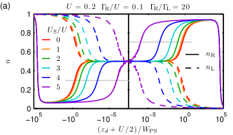
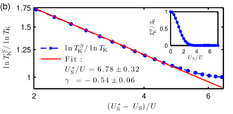
Figure 11: (Color online) Population switching for the charge sensor model of Eq. (V.1). (a) $n_{\rm R}(\varepsilon_{\!d})$ (solid lines) and $n_{\rm L}(\varepsilon_{\!d})$ (dashed lines) for several values of $U_{\rm S}/U$, plotted versus $(\varepsilon_{\!d}+U/2)/W_{\rm PS}$ in a pseudo-logarithmic fashion (“pseudo” in that the x-axis is plotted logarithmic with positive and negative values to the left and right of the switching point, respectively, represented by the vertical solid line). The horizontal light solid lines indicate the values of $n_{\rm R}$ which define the widths $W_{\rm PS}^{\rm S}$ of the PS regimes. The noisy behaviour of the curves for $U_{\rm S}=5U$ at small values of $\varepsilon_{\!d}$ indicates that our analysis cannot resolve smaller values for $\varepsilon_{\!d}$ as we are reaching the limits of double precision numerical accuracy. (b) Inset: $T_{\rm K}^{\rm S}/T_{\rm K}$ as function of $U_{\rm S}/U$, showing the rapid decrease of the Kondo temperature with increasing coupling. Main panel: $\ln T_{\rm K}^{\rm S}/\ln T_{\rm K}$ versus $(U_{\rm S}^{*}-U_{\rm S})/U$, plotted on a log-log scale (dashed line with dots), together with a linear fit using Eq. (59) (solid line).

GBG proposed to extend the asymmetric SIAM studied above by introducing a third lead as “charge sensor” for the left dot (see Fig. 10). For simplicity, it is taken to have the same density of states as the other two leads, but in contrast to the latter, it couples to the left dot only electrostatically (not by tunnelling), with interaction strength $U_{\rm S}$ (with $\hat{c}_{\rm S}\equiv\sum_{\varepsilon}\hat{c}_{\varepsilon\rm S}$):

$$\hat{H} = \hat{H}_{\rm SIAM}$$

$$+\sum_{\varepsilon}\varepsilon\,\hat{c}_{\varepsilon\rm S}^{\dagger}\hat{c}_{\varepsilon\rm S}^{{\phantom{\dagger}}}+U_{\rm S}(\hat{d}_{\rm L}^{\dagger}\hat{d}_{\rm L}^{{\phantom{\dagger}}}-\frac{1}{2})(\hat{c}_{\rm S}^{\dagger}\hat{c}_{\rm S}^{{\phantom{\dagger}}}-\frac{1}{2})\>.$$

A plot of $n_{\rm L}$ and $n_{\rm R}$ as functions of $\varepsilon_{\!d}$ for this model looks essentially similar to Fig. 7(b), showing population switching at $\varepsilon_{\!d}=-U/2$. However, when the strength of the coupling $U_{\rm S}$ is increased, the width of the PS, say $W_{\rm PS}^{\rm S}$, is strongly reduced below the value $W_{\rm PS}$ it had for $U_{\rm S}=0$, as predicted by GBG. This is illustrated in Fig. 11(a), which shows $n_{\rm R}$ (solid lines) and $n_{\rm L}$ (dashed lines) as functions of $(\varepsilon_{\!d}+U/2)/W_{\rm PS}$, using a logarithmic scale to zoom in on the immediate vicinity of the PS. In fact, as $U_{\rm S}$ approaches a critical value $U_{\rm S}^{*}$, the width $W_{\rm PS}^{\rm S}$ drops exponentially towards zero, until it becomes too small to be resolved within double precision numerical accuracy.

The behaviour of $W_{\rm PS}^{\rm S}$ is mimicked by that of the Kondo temperature, calculated via the pseudospin susceptibility, $T_{\rm K}^{\rm S}\equiv 1/\chi_{s}$. We find that it decreases relative to its $U_{\rm S}=0$ value $T_{\rm K}$, precisely in proportion to $W_{\rm PS}^{\rm S}$, such that

$$\frac{T_{\rm K}^{\rm S}}{T_{\rm K}}=\frac{W_{\rm PS}^{\rm S}}{W_{\rm PS}}$$ (58)

holds within our numerical accuracy.

The transition from a continuous to an abrupt PS as $U_{\rm S}$ crosses $U_{\rm S}^{\ast}$ has been predicted to be of the Kosterlitz-Thouless type. Goldstein2010 ; Goldstein2011 This implies that $T_{\rm K}^{\rm S}$ is expected to approach zero according to

$$-\ln T_{\rm K}^{\rm S}\sim\left(U_{\rm S}^{*}-U_{\rm S}\right)^{\gamma}\>,$$ (59)

where $\gamma=-1/2$. To test whether our data is conform to this expectation, Fig. 11(b) shows $\ln(T_{\rm K}^{\rm S})/\ln(T_{\rm K})$ vs. $(U_{\rm S}^{\ast}-U)$ on a log-log plot. Indeed, we find a straight line for $U_{\rm S}$ not too close to $U_{\rm S}^{\ast}$, consistent with Eq. (59). We extract the values $\gamma=-0.54\pm 0.06$ and $U_{\rm S}^{\ast}/U=6.78\pm 0.32$, by making linear fits over several somewhat different fitting ranges and taking the average and standard deviation of the fit parameters as final fitting results. The relatively large errors of about $10\%$ are a consequence of the fact that it is not possible to obtain data for $U_{\rm S}$ closer to $U_{\rm S}^{*}$, since this would drive $T_{\rm K}^{\rm S}$ below the level of numerical noise.

We note that analytical calculations based on Refs. Goldstein2010, and Goldstein2011, [using the more accurate criterion, $J_{z}(U_{\rm S}^{\ast})=J_{xy}(U_{\rm S}^{\ast})$ in the notation of these papers] predict the critical interaction to be $U_{\rm S}^{\ast}/U\sim 7.6$. The agreement of this prediction with the numerical result of $6.8$ is quite respectable, given the inaccuracies in both the numerical and analytical calculations [for the latter, inaccuracies arise since the cutoff scheme employed in the analytical calculation is different from the one realized numerically. The cutoff appears explicitly in the arguments of the functions $Q$ in Eqs. (6) to (10) of Ref. Goldstein2010, ].

Though the above results unambiguously show that the width of PS decreases exponentially as $U_{\rm S}$ approaches a critical value $U_{\rm S}^{\ast}$, an analysis based purely on $W_{\rm PS}^{\rm S}$ can not access the critical point itself or the regime beyond. We therefore proceed now with a numerical calculation of the dynamics of the pseudospin-flip operator, for which we are not constrained to $U_{\rm S}<U_{\rm S}^{\ast}$.

V.2 AO in dynamics of pseudospin-flip operator

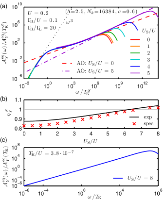
Figure 12: (Color online) (a) The pseudospin-flip spectral function $\mathcal{A}_{Y}^{\rm eq}(\omega)$ [cf. Eq. (53)] for the PS model with charge sensor, for several values of $U_{\rm S}/U$, calculated at $\varepsilon_{\!d}=-U/2$: plotting $\mathcal{A}^{\rm eq}_{Y}(\omega)/\mathcal{A}^{\rm eq}_{Y}(T_{\rm K}^{\rm S})$ versus $\omega/T_{\rm K}^{\rm S}$ yields a scaling collapse. The general shape of the curves is similar to those shown in Fig. 8: for $\omega<T_{\rm K}^{\rm S}$ we find Fermi liquid behaviour, $\sim\omega^{3}$ (dotted line), while for $\omega>T_{\rm K}^{\rm S}$ each curve shows a nontrivial AO power-law, $\sim\omega^{-1+2\eta_{Y}^{\rm S}}$ [cf. Eq. (54)], exemplified by the dashed and dash-dotted lines for $U_{\rm S}/U=0$ and $5$, respectively. (b) Comparison of the values for $\eta_{Y}^{\rm S}$ expected from Eq. (60) (solid line), or extracted from the spectral function $\mathcal{A}_{Y}^{\rm eq}(\omega)$ in the intermediate-frequency regime between $T_{\rm K}$ and the high frequency maximum (crosses). The relative errors are below $5\%$, where the errors decrease with increasing $U_{\rm S}$ for similar reasons as in Fig. 8. The light horizontal line indicates $\eta_{Y}^{\rm S}=1$. (We were unable to obtain reliable data for $U_{\rm S}$ around $7U$, presumably because this is too close to $U_{\rm S}^{\ast}$.) (c) $\mathcal{A}_{Y}^{\rm eq}(\omega)/\mathcal{A}_{Y}^{\rm eq}(T_{\rm K})$ versus $\omega/T_{\rm K}$ for $U_{\rm S}=8U$. The AO power-law behaviour $\omega^{-1+2\eta_{Y}^{S}}$ extends down to the smallest frequencies accessible, illustrating that the crossover scale $T_{\rm K}^{\rm S}$ has become undetectably small.

The reason for the $U_{\rm S}$-dependence of $W_{\rm PS}$ and $T_{\rm K}^{\rm S}$ is that the introduction of the sensor ($U_{\rm S}\neq 0$) increases the influence of AO in the leads. As pointed out by GBG, the scaling dimension of $\hat{Y}$ acquires an extra contribution $\tfrac{1}{2}\Delta_{\rm S}^{2}$ due to the sensor lead:

$$\eta_{Y}^{\rm S}=\tfrac{1}{2}(\Delta_{\rm L}+1)^{2}+\tfrac{1}{2}(-\Delta_{\rm R}-1)^{2}+\tfrac{1}{2}\Delta_{\rm S}^{2}\>,$$ (60)

where $\Delta_{\rm S}$ is given by Eq. (38), with $U_{\rm S}$ replacing $U$. By increasing $U_{\rm S}$ and thereby $\Delta_{\rm S}^{2}$, it is thus possible to drive $\eta_{Y}^{\rm S}$ beyond $1$. This will render the pseudospin-flip operators $\hat{Y}$ and $\hat{Y}^{\dagger}$ irrelevant, thus suppressing quantum fluctuations between the (0,1) and (1,0) configurations, and, hence, pushing $T_{\rm K}^{\rm S}$ down to zero.

To check this scenario explicitly, we have studied the $U_{\rm S}$-dependence of $\eta_{Y}^{\rm S}$ by extracting it from the spectral function $\mathcal{A}^{\rm eq}_{Y}(\omega)$, calculated at the particle-hole symmetric point for several values of $U_{\rm S}$. The general shape of $\mathcal{A}^{\rm eq}_{Y}$, shown in Fig. 12(a), is similar to that of Fig. 8(a) for $U_{\rm S}=0$: For frequencies well below $T_{\rm K}^{\rm S}$, $\mathcal{A}^{\rm eq}_{Y}(\omega)$ scales as $\omega^{3}$, while in the regime of intermediate frequencies, $T_{\rm K}^{\rm S}\lesssim\omega\lesssim\omega_{\rm he}$ (cf. Sec. IV.2), the spectrum shows AO power-law behaviour, $\sim\omega^{-1+2\eta_{Y}^{\rm S}}$. Indeed, Fig. 12(b) shows that the values for $\eta_{Y}^{\rm S}$ extracted from the spectra (crosses) agree fairly well with those expected from Eq. (60). Moreover, for sufficiently large $U_{\rm S}/U$, the exponents $\eta_{Y}^{\rm S}$ increase past 1, confirming that the pseudospin-flip operators become irrelevant.

V.3 AO induced by quench of level positions

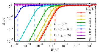
Figure 13: (Color online) AO for the PS model with charge sensing. The exponent $\Delta_{\rm AO}$ [extracted from Eq. (1)] (solid lines with dots) is shown as function of quench size $W/U$ [Eq. (55)], for several values of $U_{\rm S}/U$, with fixed values of $\Gamma_{\!\rm R}$ and $\Gamma_{\!\rm L}$. We see that $T_{\rm K}^{\rm S}/b_{0}$ (indicated by dashed vertical lines) is pushed to zero as $U_{\rm S}$ increases past $U_{\rm S}^{\ast}/U\simeq 6.78$. Already for $U_{\rm S}/U\geq 6$ the curves are essentially indistinguishable, in that they do not deviate from their constant value for all $W/U$-values accessible to our analysis. For $W\gg T_{\rm K}^{\rm S}/b_{0}$ the exponent $\Delta_{\rm AO}$ saturates to a maximal value given by Eq. (61). The corresponding values of $\Delta_{\rm ch}$ [from Eq. (7)] are not shown but agree with $\Delta_{\rm AO}$ with relative errors of a few percent.

To further highlight the effect of AO on $T_{\rm K}^{\rm S}$, let us consider again the quench of level position [Eq. (55)] studied in Sec. IV.3, and repeat the analysis presented there, but now for several different values of $U_{\rm S}/U$. Figure 13 shows the results for the exponent $\Delta_{\rm AO}$. For large values of $W$ the AO factor reaches its maximal value

$$\Delta_{\rm AO}^{\rm max}=\sqrt{(1)^{2}+(1)^{2}+\Delta_{\rm S}^{2}}\>.$$ (61)

This is similar to Eq. (56) for the model without sensor, but includes the additional contribution $\Delta_{\rm S}^{2}$ [given by Eq. (38), with $U_{\rm S}$ replacing $U$] from the displaced charge induced in the sensor lead by the change in local occupancy of the left dot from $n_{\rm L}=0$ to $1$.

The most important feature of Fig. 13 is the fact that the crossover scale $T_{\rm K}^{\rm S}/b_{0}$ (indicated by vertical dashed lines) is rapidly pushed to extremely small values as $U_{\rm S}/U$ is increased. Indeed, for $U_{\rm S}=8U$, which lies beyond the critical value of $U_{\rm S}^{*}/U\simeq 6.78$ discussed above, $\Delta_{\rm AO}$ is essentially pinned to its maximal value down to the smallest values of quench range $W$ that we can access numerically. This is consistent with the fact that the corresponding spectral function $\mathcal{A}_{Y}^{\rm eq}(\omega)$ at $U_{\rm S}=8U$, shown in Fig. 12(c), shows nontrivial AO power laws down to the lowest frequencies accessible, with no trace of a Fermi-liquid $\omega^{3}$. This demonstrates very clearly, if somewhat indirectly, that the PS will be abrupt for $U_{\rm S}>U_{\rm S}^{\ast}$.

V.4 Summary for PS with sensor

Let us summarize the results of this section, by way of extending the list of salient points collected in Sec. IV.4. (iv) The presence of a charge sensor reduces the crossover scale $T_{\rm K}^{\rm S}$, which reaches zero at a critical coupling $U_{\rm S}^{\ast}$ [Fig. 11]. (v) This reduction is due to the increased effect of AO in the leads, which increases the scaling dimension $\eta_{Y}^{\rm S}$ [Fig. 12]; when the latter passes 1 (corresponding to $U_{\rm S}=U_{\rm S}^{\ast}$), the pseudospin-flip operators become irrelevant and $T_{\rm K}^{\rm S}$ equals zero, rendering the PS abrupt. (vi) Correspondingly, for $U_{\rm S}>U_{\rm S}^{\ast}$, the spectrum $\mathcal{A}_{Y}^{\rm eq}(\omega)$ shows nontrivial AO power-law behaviour, $\omega^{-1+2\eta_{Y}^{\rm S}}$, all the way down to the smallest frequencies accessible [Fig. 12(c)], and a low-frequency regime showing Fermi-liquid exponents does not exist.

VI Concluding remarks

The goal of this paper was to elucidate the role of the Anderson orthogonality catastrophe in giving rise to anomalous scaling dimensions in dynamical correlation functions for quantum impurity models. To this end, we have studied several setups involving (interacting) quantum dots and (non-interacting) leads. The quantum dots and leads may be interconnected electrostatically, or also through tunnel-coupling. In our analysis we focussed on the asymptotic behaviour of various correlation functions $\mathcal{G}(t)$ and the corresponding spectral functions $\mathcal{A}(\omega)$ in the limit of long times or low frequencies, respectively. Their asymptotic behaviour could be understood via a generalized version of Hopfield’s rule, whose validity was checked and confirmed through an extensive NRG analysis. As a particular application, we performed a detailed study of population switching, both without and with a third lead that acts as a charge sensor. We confirmed a previous prediction Goldstein2010 ; Goldstein2011 that when the charge sensor is sufficiently strongly coupled, population switching can turn into an abrupt quantum phase transition.

Aside from presenting a systematic discussion of the generalized Hopfield rule, which, hopefully, will be useful for practitioners in the fields, several general features have emerged from our analysis:

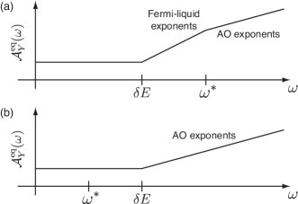
Figure 14: Schematic depiction of an equilibrium spectral function $\mathcal{A}_{Y}^{\rm eq}(\omega)$ for the cases that the local charge relaxation rate $\omega^{\ast}$ is (a) larger or (b) smaller than the lead level spacing $\delta E$.

(1) In the context of a local quantum quench of type 1, where a change of parameters switches the Hamiltonian from $\hat{H}_{\rm i}$ to $\hat{H}_{\rm f}$, each lead-dot electrostatic coupling gives rise to an AO factor in the ground state overlap $|\langle G_{{\rm i}}|G_{{\rm f}}\rangle|$, reflecting a change in the many-body configuration of the lead when the charging state of the dot is modified. This AO factor scales as $N_{\mu}^{-\frac{1}{2}\Delta_{\mu}^{2}}$, where $N_{\mu}$ is the number of electrons in lead $\mu$ and $\Delta_{\mu}$ the change in the scattering phase, divided by $\pi$, in that lead. (AO factors from leads that are not interconnected by tunnelling, so that the total charge within each channel is conserved, are multiplicative [Eq. (27)].Weichselbaum2011 )

(2) AO also arises for a type 2 quench, induced by an operator $\hat{X}^{\dagger}$ that connects initial and final ground states $|G_{\rm i}\rangle$ and $|G_{\rm f}\rangle$ lying in dynamically disconnected sectors of Hilbert space. In particular, AO influences the corresponding quench spectral function $\mathcal{A}_{X}(\omega)$ which scales as $\mathcal{A}_{X}(\omega)\sim\omega^{-1+\Delta_{\!X}^{2}}$ [Eq. (23)]. For a Hamiltonian without tunnelling terms such as the LCM of Eq. (2), the spectral function for $\hat{X}^{\dagger}=\hat{d}^{\dagger}$ thus scales as ${\mathcal{A}_{d}(\omega)\sim\omega^{-1+\Delta_{d}^{2}}}$.

(3) When a type 2 quench has the form of a tunnelling operator, $\hat{Y}^{\dagger}=\hat{c}\hat{d}^{\dagger}$, the asymptotic power law is modified to become $\mathcal{A}_{dc^{\dagger}}\sim\omega^{-1+(\Delta_{d}+1)^{2}}$ [Eq. (35c)], implying a scaling dimension $\eta^{0}_{dc^{\dagger}}=\tfrac{1}{2}(\Delta_{d}+1)^{2}$. For a particle-hole symmetric interaction term [as in Eq. (III.2)], we have $-1\leq\Delta_{d}\leq 0$ [Eq. (38)], implying that $0\leq\eta^{0}_{dc^{\dagger}}\leq 1/2$, thus tunnelling between a dot and a single lead is always a relevant perturbation.

(4) The scaling exponent can be increased, and AO strengthened, by coupling the dot(s) to further leads. In particular, leads that couple to the dot only electrostatically (not via tunnelling) contribute AO exponents of the form $\frac{1}{2}\Delta_{\mu}^{2}$, and thus enhance AO more strongly than leads that are tunnel-coupled [cf. point (3)]. In this way, the scaling dimension of the tunnelling operator can be increased past 1 [cf. Eq. (60)], and tunnelling rendered irrelevant. In such a situation, population switching becomes a quantum phase transition, tuned by gate voltage.

(5) A particularly revealing way of demonstrating the effect of AO for population switching is to calculate the exponent $\Delta_{\rm AO}$ for a type 1 quench in which the level position is abruptly changed from lying above to below the PS point (see Figs. 9 and 13, which are analogous to Fig. 6(a) for the IRLM).

(6) In the presence of tunnelling terms of the form $(\hat{c}^{\dagger}\hat{d}+\hat{d}^{\dagger}\hat{c})$, operators such as $\hat{Y}^{\dagger}=\hat{d}^{\dagger}$, $\hat{c}\hat{d}^{\dagger}$ and $\hat{c}^{\dagger}\hat{d}^{\dagger}$ do not induce a quench, since they do not cause a switch between disconnected sectors of Hilbert space. Thus, when such an operator acts on the ground state, the resulting state will relax back to the ground state over long time scales, say $t\gg 1/\omega^{\ast}$, where $\omega^{\ast}$ represents the local charge relaxation rate.

(7) The corresponding equilibrium spectral function $\mathcal{A}_{Y}^{\rm eq}(\omega)$ thus typically shows trivial Fermi-liquid exponents [e.g. Eq. (39)] in the regime of very small frequencies, $\delta E\lesssim\omega\ll\omega^{\ast}$, where $\delta E$ represents an infrared cutoff such as the level spacing in the lead. (Throughout this paper we took $\delta E\simeq 0$, since in NRG calculations $\delta E$ can be made arbitrarily small by using sufficiently long Wilson chains.)

(8) In an intermediate frequency regime $\omega>\omega^{\ast}$, the equilibrium spectral function $\mathcal{A}_{Y}^{{\rm eq}}(\omega)$ may nevertheless contain signatures of anomalous AO exponents, scaling as $\omega^{-1+2\eta^{0}_{Y}}$ [e.g. Eq. (41)], where $\eta^{0}_{Y}$ represents the scaling dimension of $\hat{Y}$ calculated in the absence of tunnelling. Thus, such exponents may be extracted by focussing on this regime of intermediate frequencies [as done in Figs. 4, 8 and 12]. This is schematically indicated in Fig. 14(a).

(9) If AO can be made so strong that the scaling dimension $\eta_{Y}^{0}$ of the operator $\hat{Y}^{\dagger}$ is larger than 1, the scale $\omega^{\ast}$ is pushed below $\delta E$ (or, in the context of NRG, below the level of numerical noise). In this case, the regime of anomalous AO scaling $\omega^{-1+2\eta^{0}_{Y}}$ will extend all the way down to the smallest frequencies accessible [e.g. 12(c)], as schematically indicated in Fig. 14(b).

To conclude, we note that cases where AO dominates in the low frequency limit such that $\omega^{\ast}\simeq 0$, [as in point (9)], quantum fluctuations of the charge on the dot(s) are essentially completely frozen out. At zero temperature and in the absence of any extraneous decay mechanism, the system will remain localized in a particular local charge configuration. Thus, varying the gate voltage in such a situation may lead to hysteretic behaviour. It would be very interesting to experimentally search for such signatures of the freezing out of charge fluctuations by performing linear response measurements at the PS point.

*

Appendix A Fermi-liquid spectral functions

In this appendix we study analytically the low energy ($\omega<\omega^{\ast}$) behaviour of the spectral functions of the IRLM (Sec. III.2) and the PS setup (Sections IV.2 and V.2).

Let us start from the noninteracting resonant level (Eq. (III.2) with $U=0$). In that case an elementary calculation gives for the retarded dot Green function, Mahan

$$\mathcal{G}_{d}^{R}(\omega)=\frac{1}{\omega-\varepsilon_{\!d}-\frac{\Gamma}{\pi\rho}\mathcal{G}_{c}^{R,0}(\omega)}=\frac{1}{\omega-\varepsilon_{\!d}+i\Gamma}\>,$$ (62)

where $\mathcal{G}_{c}^{R,0}$ is the retarded $c$ Green function for $\Gamma=0$, and we assumed the wide band limit (used just to simplify expressions, but actually not essential for any of the following arguments) $\mathcal{G}_{c}^{R,0}(\omega)=-i\pi\rho=-i\pi/2$ in units where $D=1$. The imaginary part of the retarded Green function gives (up to a factor of $-1/\pi$) the well-known Lorentzian spectral function

$$\mathcal{A}_{d}^{\rm eq}(\omega)=\frac{1}{\pi}\frac{\Gamma}{(\omega-\varepsilon_{\!d})^{2}+\Gamma^{2}}\>.$$ (63)

Thus, at low energies ($\omega\ll\Gamma$) $\mathcal{A}_{d}^{\rm eq}(\omega)$ becomes a constant, corresponding to $\eta_{d}^{\rm eq}=1/2$ [which reproduces Eq. (39a)]. This behaviour is easy to understand: In the absence of tunnelling $\mathcal{A}_{c}^{{\rm eq},0}(\omega)=\rho$ is constant, reflecting the constant local density of states of the lead electrons near the end of the lead. In the presence of tunnelling, at low energy the dot level is well-hybridized with the lead, and assumes the role of the end of the lead, thus featuring the slowly-varying low-energy spectral function $\mathcal{A}_{d}^{\rm eq}(\omega)$.

Based on similar arguments, one would expect that, in the presence of tunnelling, $\mathcal{A}_{c}^{\rm eq}(\omega)$ is still constant at low-energies, since in that limit the small spatial separation between the dot and the end of the lead should be unimportant. However, commensurability at half filling (particle-hole symmetry) makes things bit more complicated. An explicit calculation gives:

$$\mathcal{G}_{c}^{R}(\omega) = \mathcal{G}_{c}^{R,0}(\omega)+\mathcal{G}_{c}^{R,0}(\omega)\sqrt{\frac{\Gamma}{\pi\rho}}\mathcal{G}_{d}^{R}(\omega)\sqrt{\frac{\Gamma}{\pi\rho}}\mathcal{G}_{c}^{R,0}(\omega)$$ (64)

$$= -i\pi\rho\frac{\omega-\varepsilon_{\!d}}{\omega-\varepsilon_{\!d}+i\Gamma}\>.$$

Thus, when $\varepsilon_{\!d}$ is nonzero, we indeed get a constant low energy limit, i.e. $\eta_{c}^{\rm eq}=1/2$. However, when $\varepsilon_{\!d}=0$ (the value used throughout this paper for the IRLM), $\mathcal{G}_{c}^{R}(\omega)\sim\omega$ while $\mathcal{A}_{c}^{\rm eq}(\omega)\sim\omega^{2}$, corresponding to $\eta_{c}^{\rm eq}=3/2$. To understand this behaviour, let us examine a half infinite tight-binding chain with lattice spacing $a$ and Hamiltonian $\hat{H}_{\rm TB}=\sum_{n=1}^{\infty}(\hat{\Psi}_{n+1}^{\dagger}\hat{\Psi}_{n}^{{\phantom{\dagger}}}+\rm{h.c.})$. Taking the continuum limit in the standard way, we can expand the fast-varying annihilation operators $\Psi_{n}$ in terms of slowly-varying (on the scale of the Fermi wavelength) right/left moving fields $\psi_{R/L}(x)$, with $x=na$:

$$\Psi_{n}=e^{ik_{\rm F}na}\psi_{R}(na)+e^{-ik_{\rm F}na}\psi_{L}(na)\>,$$ (65)

where $k_{\rm F}$ is the Fermi wavevector. From the boundary condition $\Psi_{0}=0$ one gets $\psi_{L}(0)=-\psi_{R}(0)$, so we can define the single slowly-varying field $\psi(x)$ by $\psi(x)=\psi_{R}(x)$ if $x>0$ and $\psi(x)=-\psi_{L}(-x)$ if $x<0$. Then:

$$\Psi_{n}=e^{ik_{\rm F}na}\psi(na)-e^{-ik_{\rm F}na}\psi(-na)\>.$$ (66)

At half filling, $k_{\rm F}a=\pi/2$, we get at the site next to the boundary

$$\Psi_{n=2}=-\psi(2a)+\psi(-2a)\sim-4a\partial_{x}\psi(0)\>,$$ (67)

The same thing happens at the first site ($n=1$) when we attach a dot, since at low energies the dot behaves as the new first site. The spatial derivative is equivalent to a time derivative, up to the Fermi velocity $v_{\rm F}$. This extra time derivative is responsible for the vanishing of the spectral function $\mathcal{A}_{c}^{\rm eq}(\omega)$ for $\omega\to 0$. Since we have derivative for both $\hat{c}$ and $\hat{c}^{\dagger}$ in the Green function, and each gives an extra factor of $\omega$, we end up with $\mathcal{A}_{c}^{\rm eq}(\omega)\sim\omega^{2}$. This behaviour depends on being at half filling (particle-hole symmetry), hence is modified when $\varepsilon_{\!d}$ is not zero.

Now we can discuss the higher spectral functions, $\mathcal{A}_{dc^{\dagger}}^{\rm eq}(\omega)$, and $\mathcal{A}_{dc}^{\rm eq}(\omega)$. These are the imaginary parts of the corresponding retarded Green functions, up to a factor of $-1/\pi$. The retarded Green functions are in turn the analytical continuation of the temperature Green functions to the real frequency axis. And the temperature Green functions can be found in the noninteracting case using Wick’s theorem. Mahan

Performing these calculations for $\mathcal{A}_{dc^{\dagger}}^{\rm eq}(\omega)$, one gets:

$$\mathcal{A}_{dc^{\dagger}}^{\rm eq}(\omega) = \frac{\rho}{\pi}\Im\left[\ln\frac{\omega-\varepsilon_{\!d}+i\Gamma}{-\varepsilon_{\!d}+i\Gamma}\right.$$

$$\left.-\frac{\Gamma^{2}}{\omega(\omega+2i\Gamma)}\ln\frac{\varepsilon_{\!d}^{2}-(\omega+i\Gamma)^{2}}{\varepsilon_{\!d}^{2}+\Gamma^{2}}\right]\>.$$

Concentrating on $\omega\ll\Gamma$ one finds $\eta_{dc^{\dagger}}^{\rm eq}=\eta_{c}^{\rm eq}+\eta_{d}^{\rm eq}=1$ for $\varepsilon_{\!d}\neq 0$ and $\eta_{dc^{\dagger}}^{\rm eq}=\eta_{c}^{\rm eq}+\eta_{d}^{\rm eq}=2$ for $\varepsilon_{\!d}=0$ [the data in Fig. 4(c) corresponds to the latter case, which reproduces Eq. (39c)]. This simple summation of scaling dimensions is natural here, since there is only one possible different-time Wick-pairing, of each single-particle operator with its conjugate.

For $\mathcal{A}_{dc}^{\rm eq}(\omega)$, however, there are two different-time Wick-pairings, causing cancellations, and resulting in:

$$\mathcal{A}_{dc}^{\rm eq}(\omega)=\frac{\rho}{\pi}\Im\left[\frac{\omega-2\varepsilon_{\!d}+2i\Gamma}{\omega-2\varepsilon_{\!d}}\ln\frac{\omega-\varepsilon_{\!d}+i\Gamma}{-\varepsilon_{\!d}+i\Gamma}\right]\>.$$ (69)

Concentrating again on $\omega\ll\Gamma$ one finds now that $\eta_{dc}^{\rm eq}=2$ for all values of $\varepsilon_{\!d}$ [which reproduces Eq. (39c)].Goldstein2010b The reason is that in the low-energy continuum limit the product $\hat{d}\hat{c}$ becomes the product of annihilation operators at almost the same point. Hence, one should expand in the distance between $\hat{d}$ and $\hat{c}$ (lattice spacing). The leading term (with no spatial derivatives) vanishes by Pauli’s principle; the next term involves a spatial derivative, leading to a factor of $\omega$, similarly to the arguments above. Another factor of $\omega$ comes from the operator $\hat{c}^{\dagger}\hat{d}^{\dagger}$ appearing in the definition of $\mathcal{G}_{dc}^{\rm eq}(\omega)$. Thus, at low energies we end up with $\mathcal{A}_{dc}^{\rm eq}(\omega)\sim\omega^{3}$ even for $\varepsilon_{\!d}\neq 0$.

Although the above calculations were performed for the noninteracting case, the qualitative arguments explaining the low-energy behaviour are valid even when $U>0$. Moreover, since the system flows to the same fixed point for all values of $U>0$, the low energy power-laws are in any case independent of $U$. Our numerical results (Fig. 4) are in agreement with this picture.

Let us now turn to the low-energy behaviour of the PS setup in the case where PS is continuous. At low-energy the system is governed by Kondo physics, Eq. (49), Kashcheyevs2007 ; Lee2007 ; Silvestrov2007 ; Kashcheyevs2009 where the L-R degree of freedom plays the role of a pseudo-spin. The equivalence to Kondo continues to hold even in the presence of a charge sensor, as shown by GBG. Goldstein2010 ; Goldstein2011 The operator $\hat{Y}=\hat{d}_{R}^{\dagger}\hat{d}_{L}^{{\phantom{\dagger}}}\hat{c}_{R}^{{\phantom{\dagger}}}\hat{c}_{L}^{\dagger}$ (which is relevant in the continuous-PS phase) is the pseudospin-flip local exchange term between the dot and the lead. Similarly, the IRLM is also equivalent to the Kondo model, Gogolin ; Schlottmann1980 ; Borda2008 with the role of spin replaced by the charging state of the dot. The pseudo-spin local exchange term is simply $\hat{d}\hat{c}^{\dagger}$. Hence, when the parameters are properly mapped, the spectral functions $\mathcal{A}_{Y}^{\rm eq}(\omega)$ and $\mathcal{A}_{dc^{\dagger}}^{\rm eq}(\omega)$ are equivalent when the Kondo description applies (i.e. for $\omega\ll D$ for the IRLM, and $\omega\ll\omega_{\rm he}$ for the PS setup). In particular, $\mathcal{A}_{Y}^{\rm eq}(\omega)$ should exhibit an $\omega^{3}$ behaviour at low energy, similarly to $A_{dc^{\dagger}}^{\rm eq}(\omega)$ for $\varepsilon_{\!d}=0$, as the NRG data shows [dotted line in Fig. 8(a) and Fig. 12(a)].

References

- (1) P. W. Anderson, Phys. Rev. Lett. 18, 1049 (1967).
- (2) K. D. Schotte and U. Schotte, Phys. Rev. 185, 509 (1969).
- (3) G. D. Mahan, Phys. Rev. 163, 612 (1967).
- (4) J. J. Hopfield, Comments Solid State Phys. 2, 40 (1969).
- (5) B. Roulet, J. Gavoret, and P. Nozières, Phys. Rev. 178, 1072 (1969); P. Nozières, J. Gavoret, and B. Roulet, Phys. Rev. 178, 1084 (1969); P. Nozières, and C. T. De Dominics, Phys. Rev. 178, 1097 (1969).
- (6) B. L. Altshuler and A. G. Aronov, Pis’ma Zh. Eksp. Teor. Fiz. 30, 514 (1979).
- (7) A. O. Gogolin, Phys. Rev. Lett. 71, 2995 (1993).
- (8) N. V. Prokof’ev, Phys. Rev. B 49, 2148 (1994).
- (9) I. Affleck and A. W. W. Ludwig, J. Phys. A 27, 5375 (1994).
- (10) A. Furusaki, Phys. Rev. B 56, 9352 (1997).
- (11) A. O. Gogolin, A. A. Nersesyan, and A. M. Tsvelik, Bosonization and Strongly Correlated Systems (Cambridge University Press, Cambridge, 2004).
- (12) A. J. Leggett, S. Chakravarty, A. T. Dorsey, M. P. A. Fisher, A. Garg, W. Zwerger, Rev. Mod. Phys. 59, 1 (1987).
- (13) Z. Ovadyahu, Phys. Rev. Lett. 99, 226603 (2007).
- (14) R. W. Helmes, M. Sindel, L. Borda, and J. von Delft, Phys. Rev. B 72, 125301 (2005).
- (15) H. E. Türeci, M. Hanl, M. Claassen, A. Weichselbaum, T. Hecht, B. Braunecker, A. Govorov, L. Glazman, A. Imamoglu, and J. von Delft, Phys. Rev. Lett. 106, 107402 (2011).
- (16) C. Latta, F. Haupt, M. Hanl, A. Weichselbaum, M. Claassen, W. Wuester, P. Fallahi, S. Faelt, L. Glazman, J. von Delft, H. E. Türeci, and A. Imamoglu, Nature 474, 627 (2011).
- (17) M. Goldstein, R. Berkovits, and Y. Gefen, Phys. Rev. Lett. 104, 226805 (2010).
- (18) M. Goldstein, Y. Gefen, and R. Berkovits, Phys. Rev. B 83, 245112 (2011).
- (19) K. G. Wilson, Rev. Mod. Phys. 47, 773 (1975).
- (20) R. Bulla, T. A. Costi, and T. Pruschke, Rev. Mod. Phys. 80, 395 (2008).
- (21) A. Weichselbaum, W. Münder, and J. von Delft, Phys. Rev. B 84, 075137 (2011).
- (22) J. Friedel, Phil. Mag. 43, 153 (1952).
- (23) J. Friedel, Can. J. Phys. 34, 1190 (1956).
- (24) D. C. Langreth, Phys. Rev. 150, 516 (1966).
- (25) A. C. Hewson, The Kondo problem to heavy Fermions (Cambridge University Press, Cambridge, 1993).
- (26) Compare Ref. Friedel1952, , p. 159; Ref. Friedel1956, , Eq. (7); Ref. Langreth1966, , Eq. (21); Ref. Hewson, , Sec. 1.2.
- (27) O. Gunnarsson and K. Schönhammer, Phys. Rev. B 28, 4315 (1983).
- (28) J. Cardy, Scaling and Renormalization in Statistical Physics (Cambridge University Press, Cambridge, 1996).
- (29) L. N. Oliveira and J. W. Wilkins, Phys. Rev. B 24, 4863 (1981); D. L. Cox, H. O. Frota, L. N. Oliveira, and J. W. Wilkins, Phys. Rev. B 32, 555 (1985).
- (30) T. A. Costi, P. Schmitteckert, J. Kroha, and P. Wölfle, Phys. Rev. Lett. 73, 1275 (1994).
- (31) F. B. Anders and A. Schiller, Phys. Rev. Lett. 95, 196801 (2005).
- (32) F. B. Anders and A. Schiller, Phys. Rev. B 74, 245113 (2006).
- (33) R. Peters, T. Pruschke and F. B. Anders, Phys. Rev. B 74, 245114 (2006).
- (34) A. Weichselbaum and J. von Delft, Phys. Rev. Lett. 99, 076402 (2007).
- (35) P. Schlottmann, Phys. Rev. B 22, 622 (1980).
- (36) L. Borda, A. Schiller, and A. Zawadowski, Phys. Rev. B 78, 201301 (2008).
- (37) M. Goldstein, Y. Weiss, and R. Berkovits, Europhys. Lett. 86, 67012 (2009); Physica E 42, 610 (2010).
- (38) M. Goldstein and R. Berkovits, Phys. Rev. B 82, 235315 (2010).
- (39) G. Hackenbroich, W. D. Heiss, and H. A. Weidenmüller, Phys. Rev. Lett. 79, 127 (1997).
- (40) R. Baltin, Y. Gefen, G. Hackenbroich and H. A. Weidenmüller, Eur. Phys. J. B 10, 119 (1999).
- (41) P. G. Silvestrov and Y. Imry, Phys. Rev. Lett. 85, 2565 (2000).
- (42) P. G. Silvestrov and Y. Imry, Phys. Rev. B 65, 035309 (2001).
- (43) D. I. Golosov and Y. Gefen, Phys. Rev. B 74, 205316 (2006).
- (44) C. Karrasch, T. Hecht, A. Weichselbaum, Y. Oreg, J. von Delft, and V. Meden, Phys. Rev. Lett. 98, 186802 (2007).
- (45) V. Kashcheyevs, A. Schiller, A. Aharony, and O. Entin-Wohlman, Phys. Rev. B 75, 115313 (2007).
- (46) H. W. Lee and S. Kim, Phys. Rev. Lett. 98, 186805 (2007).
- (47) P. G. Silvestrov and Y. Imry, Phys. Rev. B 75, 115335 (2007).
- (48) V. Kashcheyevs, C. Karrasch, T. Hecht, A. Weichselbaum, V. Meden, and A. Schiller, Phys. Rev. Lett. 102, 136805 (2009).
- (49) G. D. Mahan, Many-Particle Physics (Kluwer, New York, 2000).