Graph colorings, flows
and
arithmetic Tutte polynomial

Abstract.

We introduce the notions of arithmetic colorings and arithmetic flows over a graph with labelled edges, which generalize the notions of colorings and flows over a graph.

We show that the corresponding arithmetic chromatic polynomial and arithmetic flow polynomial are given by suitable specializations of the associated arithmetic Tutte polynomial, generalizing classical results of Tutte [7].

Introduction

It is well known how to associate a matroid, and hence a Tutte polynomial, to a graph. Moreover, several combinatorial objects associated to a graph are counted by suitable specializations of this important invariant: (proper) $q$-colorings and (nowhere zero) $q$-flows are two of the most classical examples. See [4] and [8] for systematic accounts.

In [5] a new polynomial has been introduced, which provides a natural counterpart for toric arrangements of the Tutte polynomial of a hyperplane arrangement. In fact in [5] and [1] it has been shown how this polynomial has several applications to toric arrangements, vector partition functions and zonotopes.

In [2] we introduced the notion of an arithmetic matroid, which generalizes the one of a matroid, and whose main example is provided by a list of elements in a finitely generated abelian group. To this object we associated an arithmetic Tutte polynomial (which is the polynomial in [5] for the main example) and provided a combinatorial interpretation of it which extends the one given by Crapo for the classical Tutte polynomial.

Encouraged by all these evidences (cf. also [3] where two parallel theories are developed), we think of the arithmetic matroids and the arithmetic Tutte polynomial as natural generalizations of their classical counterparts. So it seemed also natural to us to look for applications in graph theory.

In this paper we introduce the notion of an arithmetic (proper) $q$-coloring and an arithmetic (nowhere zero) $q$-flow over a graph $(\mathcal{G},\ell)$ with labelled (by integers) edges, which generalize the well known notions of $q$-colorings and $q$-flows of a graph. We then associate to the labelled graph an arithmetic matroid $\mathfrak{M}_{\mathcal{G},\ell}$, and we show how suitable specializations of its arithmetic Tutte polynomial provides the arithmetic chromatic polynomial $\chi_{\mathcal{G},\ell}(q)$ and the arithmetic flow polynomial $\chi_{\mathcal{G},\ell}^{*}(q)$ of the labelled graph (see Theorem 3.1 and Theorem 5.2).

These can be seen as generalizations of the classical results of Tutte [7] (Corollaries 3.2 and 5.3) that the chromatic polynomial and the flow polynomial of a graph can be obtained as suitable specializations of the corresponding Tutte polynomial.

The paper is organized in the following way.

In the first section we define the basic notions of graph theory that we need, in particular the notion of labelled graph, and we fix the corresponding notation.

In the second section we recall some basic notions of the theory of arithmetic matroids. In particular we state some of their basic properties, and we show how to associate to a labelled graph an arithmetic matroid.

In the third section we introduce the notion of arithmetic coloring and we state Theorem 3.1.

In the fourth section we prove Theorem 3.1.

In the fifth section we introduce the notion of arithmetic flow and we state Theorem 5.2.

In the sixth section we prove Theorem 5.2.

In the last section we make some final comments and we formulate an open problem.

Acknowledgments

We would like to thank Petter Brändén and Matthias Lenz for interesting discussions.

1. Labelled graphs

In this paper a graph $\mathcal{G}$ will be a pair $(V,E)$, where $V$ is a finite set whose elements are called vertices, and $E$ is a finite multiset of 2-element multisets of $V$, which are called edges. A loop is an edge whose elements coincide.

In this paper we will always assume that our graphs have no loops.

Example 1.1.

Consider $\mathcal{G}:=(V,E)$, where $V:=\{v_{1},v_{2},v_{3},v_{4}\}$ is the set of vertices and $E:=\{\{v_{1},v_{2}\}$, $\{v_{2},v_{3}\}$, $\{v_{2},v_{4}\}$, $\{v_{3},v_{4}\}\}$ is the set of edges (see Figure 1).

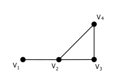
Figure 1. The graph $\mathcal{G}$.

We define the classical deletion of an edge $e$ of a graph $\mathcal{G}=(V,E)$ to be simply the graph $(V,E\backslash\{e\})$, i.e. the graph $\mathcal{G}$ with the edge $e$ removed.

We define the classical contraction of an edge $e$ of a graph $\mathcal{G}=(V,E)$ to be the graph $\mathcal{G}$ with the edge $e$ removed and with the corresponding vertices identified.

Example 1.2.

Let $\mathcal{G}:=(V,E)$, where $V:=\{v_{1},v_{2},v_{3},v_{4}\}$ is the set of vertices and $E:=\{\{v_{1},v_{2}\}$, $\{v_{2},v_{3}\}$, $\{v_{2},v_{4}\}$, $\{v_{3},v_{4}\}\}$ is the set of edges. Let $e:=\{v_{2},v_{3}\}\in E$. Then the classical deletion of $e$ is the graph with vertices $V$, and edges $E\setminus e=\{\{v_{1},v_{2}\},\{v_{2},v_{4}\},\{v_{3},v_{4}\}\}$, while the classical contraction of $e$ is the graph with vertices $V^{\prime}:=\{v_{1}^{\prime},v_{2}^{\prime},v_{3}^{\prime}\}$ and edges $E^{\prime}:=\{\{v_{1}^{\prime},v_{2}^{\prime}\}$, $\{v_{2}^{\prime},v_{3}^{\prime}\}$, $\{v_{2}^{\prime},v_{3}^{\prime}\}\}$ (see Figure 2).

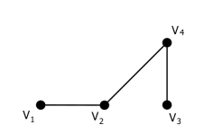
(a) Classical deletion of $e$

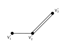
(b) Classical contraction of $e$

Figure 2. The classical deletion and contraction of $e$

We distinguish two kinds of edges: we assume that $E$ is a disjoint union $E=R\cup D$, where we call the elements of $R$ regular edges, while we call the elements of $D$ dotted edges.

A labelled graph in this contest will be simply a pair $(\mathcal{G},\ell)$, where $\mathcal{G}=(V,E)$ is a graph, and $\ell:E\rightarrow\mathbb{N}\setminus\{0\}$ is a map, whose images are called labels of the corresponding edges.

Example 1.3.

Consider $(\mathcal{G},\ell)$, where $\mathcal{G}:=(V,E)$, $V:=\{v_{1},v_{2},v_{3},v_{4}\}$ is the set of vertices, $R:=\{\{v_{1},v_{2}\},\{v_{2},v_{3}\},\{v_{2},v_{4}\}\}$ the set of regular edges, $D:=\{\{v_{3},v_{4}\}\}$ the set of dotted edges, so that $E=R\cup D=\{\{v_{1},v_{2}\},\{v_{2},v_{3}\},\{v_{2},v_{4}\},\{v_{3},v_{4}\}\}$. Moreover let $\ell(\{v_{1},v_{2}\})=1$, $\ell(\{v_{2},v_{3}\})=2$, $\ell(\{v_{2},v_{4}\})=3$, $\ell(\{v_{3},v_{4}\})=6$ be the labels of the edges (see Figure 3).

Figure 3. The labelled graph $(\mathcal{G},\ell)$.

A directed graph is a pair $(V,E)$ where $V$ is a finite set of vertices, and $E$ is a finite multiset of ordered pairs of elements of $V$ that we call directed edges. For a directed edge $e\in E$ we will denote by $e^{+}$ and $e^{-}$ the first and the second coordinate of $e$ respectively. Pictorially, to denote a directed edge we draw an arrow pointing toward its first coordinate.

Given a graph $\mathcal{G}=(V,E)$, an orientation $E_{\theta}=R_{\theta}\cup D_{\theta}$ of the edges $E=R\cup D$ is a multiset of ordered pairs of elements of $V$ whose underlying sets are the elements of $E$. We will call $\mathcal{G}_{\theta}$ the corresponding directed graph.

Given a labelled graph $(\mathcal{G},\ell)$, where $\mathcal{G}=(V,E)$ and $E=R\cup D$, we define the deletion of a regular edge $e\in R$ to be the pair $(\mathcal{G}-e,\ell_{1})$, where $\mathcal{G}-e=(V,E_{1})$ is the classical deletion of the edge $e$ (i.e. $E_{1}=R_{1}\cup D_{1}$, $R_{1}=R\setminus\{e\}$, $D_{1}=D$), and $\ell_{1}$ is simply the restriction of $\ell$ to $E_{1}$; we define the contraction of $e\in R$ to be the pair $(\mathcal{G}/e,\ell_{2})$, where $\mathcal{G}/e=(V,E_{2})$ is the graph obtained from $\mathcal{G}$ by removing $e$ from $R$ and putting it in $D$, i.e. making the regular edge $e$ into a dotted one (i.e $E_{2}=R_{2}\cup D_{2}$, $R_{2}=R\setminus\{e\}$, $D_{2}=D\cup\{e\}$), and $\ell_{2}$ is the same as $\ell$.

Example 1.4.

Consider $(\mathcal{G},\ell)$ as in Example 1.3. For $e:=\{v_{2},v_{3}\}\in R$ we show the deletion and the contraction of $e$ in Figure 4.

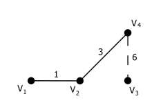
(a) Deletion of $e$

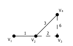
(b) Contraction of $e$

Figure 4. The deletion and the contraction of $e$

Given a graph $\mathcal{G}=(V,E)$ with $E=R\cup D$, we denote by $\overline{\mathcal{G}}=(\overline{V},\overline{E})$ the graph obtained from $\mathcal{G}$ by (classically) contracting the edges in $D$. For a regular edge $e\in R$, we will use the notation $\overline{\mathcal{G}-e}=(\overline{V}_{1},\overline{E}_{1})$ and $\overline{\mathcal{G}/e}=(\overline{V}_{2},\overline{E}_{2})$.

2. Arithmetic matroids

We recall here same basic notions of the theory of arithmetic matroids. We refer to [2] for proofs and for a more systematic treatment.

We will use the word list as a synonymous of multiset. Hence a list may contain several copies of the same element.

2.1. Matroids

A matroid $\mathfrak{M}=\mathfrak{M}_{X}=(X,rk)$ is a list of vectors $X$ with a rank function $rk:\mathbb{P}(X)\rightarrow\mathbb{N}\cup\{0\}$ which satisfies the following axioms:

1. if $A\subseteq X$, then $rk(A)\leq|A|$;

2. if $A,B\subseteq X$ and $A\subseteq B$, then $rk(A)\leq rk(B)$;

3. if $A,B\subseteq X$, then $rk(A\cup B)+rk(A\cap B)\leq rk(A)+rk(B)$.

A sublist $A$ of $X$ is called independent if $rk(A)=|A|$. It is easy to show that the independent sublists determine the matroid structure.

Example 2.1.

1. A list $X$ of vectors in a vector space, where the independent sublists are defined to be the linearly independent ones naturally form a matroid.

2. A list $X$ of edges in a graph, where the independent sublists are the edges of the subgraphs that are forests (i.e. the subgraphs without circuits) naturally form a matroid.

Given a matroid $\mathfrak{M}_{X}$ and a vector $v\in X$, we can define the deletion of $\mathfrak{M}_{X}$ as the matroid $\mathfrak{M}_{X_{1}}$, whose list of vectors is $X_{1}:=X\setminus\{v\}$, and whose independent lists are just the independent lists of $\mathfrak{M}_{X}$ contained in $X_{1}$. Notice that the rank function $rk_{1}$ of $\mathfrak{M}_{X_{1}}$ is just the restriction of the rank function $rk$ of $\mathfrak{M}_{X}$.

Given a matroid $\mathfrak{M}_{X}$ and a vector $v\in X$, we can define the contraction of $\mathfrak{M}_{X}$ as the matroid $\mathfrak{M}_{X_{2}}$, whose list of vectors is $X_{2}:=X\setminus\{v\}$, and whose rank function $rk_{2}$ is given by $rk_{2}(A):=rk(A\cup\{v\})-rk(\{v\})$, where of course $rk$ is the rank function of $\mathfrak{M}_{X}$.

Example 2.2.

1. For a matroid given by a list $X$ of vectors in a vector space, the deletion consists of removing the vector from the list, while the contraction consists of removing it from the list, taking the quotient by the subspace that it generates, and identifying the remaining vectors with their cosets.

2. For a matroid given by a list $X$ of edges in a graph, the deletion consists of removing the edge from the list, i.e. the classical deletion of the edge, while the contraction corresponds to the classical contraction of the edge.

Given two matroids $\mathfrak{M}_{X_{1}}=(X_{1},I_{1})$ and $\mathfrak{M}_{X_{2}}=(X_{2},I_{2})$, we can form their direct sum: this will be the matroid $\mathfrak{M}_{X}=\mathfrak{M}_{X_{1}}\oplus\mathfrak{M}_{X_{2}}$ whose list of vectors is the disjoint union $X:=X_{1}\sqcup X_{2}$, and where the independent lists will be the disjoint unions of lists from $I_{1}$ with lists from $I_{2}$. Hence for any sublist $A\subseteq X$, the rank $rk(A)$ of $A$ will be the sum of the rank $rk_{1}(A\cap X_{1})$ of $A\cap X_{1}$ in $\mathfrak{M}_{X_{1}}$ with the rank $rk_{2}(A\cap X_{2})$ of $A\cap X_{2}$ in $\mathfrak{M}_{X_{2}}$.

The Tutte polynomial of the matroid $\mathfrak{M}_{X}=(X,rk)$ is defined as

$$T_{X}(x,y):=\sum_{A\subseteq X}(x-1)^{rk(X)-rk(A)}(y-1)^{|A|-rk(A)}.$$

2.2. Arithmetic matroids

An arithmetic matroid is a pair $(\mathfrak{M}_{X},m)$, where $\mathfrak{M}_{X}$ is a matroid on a list of vectors $X$, and $m$ is a multiplicity function, i.e. $m:\mathbb{P}(X)\rightarrow\mathbb{N}\setminus\{0\}$ has the following properties:

• if $A\subseteq X$ and $v\in X$ is dependent on $A$, then $m(A\cup\{v\})$ divides $m(A)$;

• if $A\subseteq X$ and $v\in X$ is independent on $A$, then $m(A)$ divides $m(A\cup\{v\})$;

• if $A\subseteq B\subseteq X$ and $B$ is a disjoint union $B=A\cup F\cup T$ such that for all $A\subseteq C\subseteq B$ we have $rk(C)=rk(A)+|C\cap F|$, then

  $$m(A)\cdot m(B)=m(A\cup F)\cdot m(A\cup T).$$

• if $A\subseteq B$ and $rk(A)=rk(B)$, then

  $$\mu_{B}(A):=\sum_{A\subseteq T\subseteq B}(-1)^{|T|-|A|}m(T)\geq 0.$$

• if $A\subseteq B$ and $rk^{*}(A)=rk^{*}(B)$, then

  $$\mu_{B}^{*}(A):=\sum_{A\subseteq T\subseteq B}(-1)^{|T|-|A|}m(X\setminus T)\geq 0.$$

Example 2.3.

The prototype of an arithmetic matroid is the one that we are going to associate now to a finite list $X$ of elements of a finitely generated abelian group $G$.

Given a sublist $A\subseteq X$, we will denote by $\langle A\rangle$ the subgroup of $G$ generated by the underlying set of $A$.

We define the rank of a sublist $A\subseteq X$ as the maximal rank of a free (abelian) subgroup of $\langle A\rangle$. This defines a matroid structure on $X$.

For $A\subseteq X$, let $G_{A}$ be the maximal subgroup of $G$ such that $\langle A\rangle\leq G_{A}$ and $|G_{A}:\langle A\rangle|<\infty$, where $|G_{A}:\langle A\rangle|$ denotes the index (as subgroup) of $\langle A\rangle$ in $G_{A}$. Then the multiplicity $m(A)$ is defined as $m(A):=|G_{A}:\langle A\rangle|$.

Remark 2.1.

Notice that in $\mathbb{Z}^{m}$, to compute the multiplicity of a list of elements, it is enough to see the elements as the columns of a matrix, and to compute the greatest common divisor of its minors of order the rank of the matrix (cf. [6, Theorem 2.2]).

Given an arithmetic matroid $(\mathfrak{M}_{X},m)$ and a vector $v\in X$, we define the deletion of $(\mathfrak{M}_{X},m)$ as the arithmetic matroid $(\mathfrak{M}_{X_{1}},m_{1})$, where $\mathfrak{M}_{X_{1}}$ is the deletion of $\mathfrak{M}_{X}$ and $m_{1}(A):=m(A)$ for all $A\subseteq X_{1}=X\setminus\{v\}$.

Given an arithmetic matroid $(\mathfrak{M}_{X},m)$ and a vector $v\in X$, we define the contraction of $(\mathfrak{M}_{X},m)$ as the arithmetic matroid $(\mathfrak{M}_{X_{2}},m_{2})$, where $\mathfrak{M}_{X_{2}}$ is the contraction of $\mathfrak{M}_{X}$ and $m_{2}(A):=m(A\cup\{v\})$ for all $A\subseteq X_{2}=X\setminus\{v\}$.

We say that $v\in X$ is:

• free if both $rk_{1}(X\setminus\{v\})=rk(X\setminus\{v\})=rk(X)-1$ and $rk_{2}(X\setminus\{v\})=rk(X)-1$;

• torsion if both $rk_{1}(X\setminus\{v\})=rk(X)$ and $rk_{2}(X\setminus\{v\})=rk(X)$;

• proper if both $rk_{1}(X\setminus\{v\})=rk(X)$ and $rk_{2}(X\setminus\{v\})=rk(X)-1$.

Observe that any vector of a matroid is of one and only one of the previous three types.

Example 2.4.

In the Example 2.3, the deletion consists of removing the vector from the list, while the contraction consists of removing it from the list, taking the quotient by the subgroup that it generates, and identifying the remaining vectors with their cosets.

In this case the torsion vectors are the torsion elements in the algebraic sense, while the free vectors are the elements $v\in X$ such that $\langle X\rangle\cong\langle X\setminus\{v\}\rangle\oplus\langle v\rangle$.

Given two arithmetic matroids $(\mathfrak{M}_{X_{1}},m_{1})$ and $(\mathfrak{M}_{X_{2}},m_{2})$ we define their direct sum as the arithmetic matroid $(\mathfrak{M}_{X},m)$, where $\mathfrak{M}_{X}:=\mathfrak{M}_{X_{1}}\oplus\mathfrak{M}_{X_{2}}$, and for any sublist $A\subseteq X=X_{1}\sqcup X_{2}$, we set $m(A):=m_{1}(A\cap X_{1})\cdot m_{2}(A\cap X_{2})$.

Remark 2.2.

If the two arithmetic matroids are represented by a list $X_{1}$ of elements of a group $G_{1}$ and a list $X_{2}$ of elements of a group $G_{2}$, then, with the obvious identifications, $X:=X_{1}\sqcup X_{2}$ is a list of elements of the group $G:=G_{1}\oplus G_{2}$, and the arithmetic matroid associated to this list is exactly the direct sum of the two.

We associate to an arithmetic matroid $\mathfrak{M}_{X}$ its arithmetic Tutte polynomial $M_{X}(x,y)=M(\mathfrak{M}_{X};x,y)$ defined as

(2.1) $$M_{X}(x,y):=\sum_{A\subseteq X}m(A)(x-1)^{rk(X)-rk(A)}(y-1)^{|A|-rk(A)}.$$

2.3. Basic properties

We summarize in the following theorem some basic properties of this polynomial (cf. [2, Proofs of Lemmas 6.4, 6.6, 7.6 and Section 3.6]).

Theorem 2.1.

Let $\mathfrak{M}_{X}$ be an arithmetic matroid, and let $v\in X$ be a vector. Denote by $M_{X}(x,y)$, $M_{X_{1}}(x,y)$ and $M_{X_{2}}(x,y)$ the arithmetic Tutte polynomial associated to $\mathfrak{M}_{X}$, the deletion of $v$ and the contraction of $v$ respectively.

1. If $v$ is a proper vector then

   $$M_{X}(x,y)=M_{X_{1}}(x,y)+M_{X_{2}}(x,y).$$

2. If $v$ is a free vector then

   $$M_{X}(x,y)=(x-1)M_{X_{1}}(x,y)+M_{X_{2}}(x,y).$$

3. If $v$ is a torsion vector then

   $$M_{X}(x,y)=M_{X_{1}}(x,y)+(y-1)M_{X_{2}}(x,y).$$

4. If $\mathfrak{M}_{X}$ is the direct sum of two matroids $\mathfrak{M}_{1}$ and $\mathfrak{M}_{2}$, then

   $$M_{X}(x,y)=M(\mathfrak{M}_{1};x,y)\cdot M(\mathfrak{M}_{2};x,y).$$

2.4. A fundamental construction

We associate to each labelled graph $(\mathcal{G},\ell)$ an arithmetic matroid $\mathfrak{M}_{\mathcal{G},\ell}$ in the following way.

First of all we enumerate the vertices $V=\{v_{1},v_{2},\dots,v_{n}\}$ and we fix an orientation $E_{\theta}$ of the edges $E$. Then to each edge $e=(v_{i},v_{j})\in E_{\theta}$ we associate the element $x_{e}\in\mathbb{Z}^{n}$ defined as the vector whose $i$-th coordinate is $\ell(e)$, whose $j$-th coordinate is $-\ell(e)$, and whose other coordinates are $0$. We denote by $X_{R}$ and $X_{D}$ the multisets of vectors in $\mathbb{Z}^{n}$ corresponding to elements of $R$ and $D$ respectively.

Then we look at the group $G:=\mathbb{Z}^{n}/\langle X_{D}\rangle$, and we identify the elements of $X_{R}$ with the corresponding cosets in $G$. This gives as an arithmetic matroid $\mathfrak{M}=\mathfrak{M}_{X_{R}}=\mathfrak{M}_{\mathcal{G},\ell}$, which is clearly independent on the orientation that we choose (changing the orientation of an edge corresponds to multiply the corresponding vector in $X_{R}$ or $X_{D}$ by $-1$).

We denote by $M_{X_{R}}(x,y)=M_{\mathcal{G},\ell}(x,y)$ the associated arithmetic Tutte polynomial.

Example 2.5.

Consider $(\mathcal{G},\ell)$ as in Example 1.3 and the orientation shown in Figure 5.

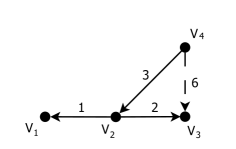
Figure 5. The labelled graph $(\mathcal{G},\ell)$ with an orientation.

We have $X_{R}=\{(1,-1,0,0),(0,-2,2,0),(0,3,0,-3)\}$$\subseteq\mathbb{Z}^{4}$ and $X_{D}=\{(0,0,6,-6)\}$ $\subseteq\mathbb{Z}^{4}$, so $G:=\mathbb{Z}^{4}/\langle(0,0,6,-6)\rangle$, and we identify $X_{R}$ with $\left\{v_{1}:=\overline{(1,-1,0,0)}\right.$, $v_{2}:=\overline{(0,-2,2,0)}$, $\left.v_{3}:=\overline{(0,3,0,-3)}\right\}\subseteq G$, where $\overline{u}$ indicates the coset of the representative $u\in\mathbb{Z}^{4}$.

We have (cf. Remark 2.1) $m(\emptyset)=m(\{v_{1}\})=m(\{v_{2},v_{3}\})=m(X_{R})=6$, $m(\{v_{2}\})=m(\{v_{1},v_{2}\})=12$, $m(\{v_{3}\})=m(\{v_{1},v_{3}\})=18$, so $M_{\mathcal{G},\ell}(x,y)=6x^{2}+18x+6xy$.

3. Arithmetic colorings

In this section we discuss the notion of arithmetic coloring.

3.1. Definitions

Given a labelled graph $(\mathcal{G},\ell)$, let $q$ be a positive integer. An arithmetic (proper) $q$-coloring of $(\mathcal{G},\ell)$ is a map $c:V\rightarrow\mathbb{Z}/q\mathbb{Z}$ that satisfies the following conditions:

1. if $u,v\in V$ and $e:=\{u,v\}\in R$, then $\ell(e)\cdot c(u)\neq\ell(e)\cdot c(v)$;

2. if $u,v\in V$ and $e:=\{u,v\}\in D$, then $\ell(e)\cdot c(u)=\ell(e)\cdot c(v)$.

For our results we will need to restrict ourself to consider only positive integers $q$ such that $\ell(e)$ divides $q$ for all $e\in E$ (cf. Remark 3.3). We will call such an integer admissible.

Remark 3.1.

For a trivial labelling $\ell\equiv 1$ and $D=\emptyset$, clearly we just recover the usual notion of (proper) $q$-coloring (any $q$ will be admissible now) of the underlying graph.

If $\ell\equiv 1$ and $D\neq\emptyset$, then we can still interpret it as a $q$-coloring, but this time of the graph $\overline{\mathcal{G}}$ (that is obtained from $\mathcal{G}$ by performing the classical contraction of all the edges in $D$).

More generally, given $\ell(e)=1$ for some $e\in D$, if we do a classical contraction of $e$, then we get a graph with the same number of arithmetic $q$-coloring.

Example 3.1.

Consider $(\mathcal{G},\ell)$ with $\mathcal{G}:=(V,E)$, $V=\{v_{1},v_{2},v_{3}\}$, $R:=\{e_{1}:=\{v_{1},v_{2}\},e_{2}:=\{v_{1},v_{2}\}\}$, $D:=\{e_{3}:=\{v_{2},v_{3}\}\}$ so $E=R\cup D=\{e_{1},e_{2},e_{3}\}$, $\ell(e_{1})=2$, $\ell(e_{2})=3$ and $\ell(e_{3})=2$ (see Figure 6).

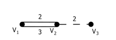
Figure 6. The labelled graph $(\mathcal{G},\ell)$.

Then any multiple of $6$ is admissible. For example for $q=6$ we denote the $6$-colorings as vectors of $(\mathbb{Z}/6\mathbb{Z})^{3}$, where for every $i=1,2,3$, the $i$-th coordinate corresponds to the color of the vertex $v_{i}$.

In this case there are $24$ possible $6$-colorings of $(\mathcal{G},\ell)$: $(\overline{a},\overline{1}+\overline{a},\overline{1}+\overline{a})$, $(\overline{a},\overline{1}+\overline{a},\overline{4}+\overline{a})$, $(\overline{a},\overline{5}+\overline{a},\overline{5}+\overline{a})$, $(\overline{a},\overline{5}+\overline{a},\overline{2}+\overline{a})$ for all $\overline{a}\in\mathbb{Z}/6\mathbb{Z}$.

We define the arithmetic chromatic polynomial of a labelled graph $(\mathcal{G},\ell)$ to be the function ${\chi}_{\mathcal{G},\ell}(\cdot):\mathbb{N}\setminus\{0\}\rightarrow\mathbb{N}\cup\{0\}$, which assigns to each positive integer $q$ the number of arithmetic $q$-colorings of $(\mathcal{G},\ell)$. We will show in Theorem 3.1 that this is in fact a polynomial function.

Remark 3.2.

For a trivial labelling $\ell\equiv 1$ and $D=\emptyset$, we just recover the usual notion of the chromatic polynomial $\chi_{\mathcal{G}}(q)$ of the underlying graph $\mathcal{G}$.

If $\ell\equiv 1$ and $D\neq\emptyset$, then we can still interpret it as a chromatic polynomial of the graph $\overline{\mathcal{G}}$.

Example 3.2.

Consider $(\mathcal{G},\ell)$ as in Example 3.1. We have $q$ choices for the color $c(v_{1})$ of $v_{1}$, $q-4$ choices for $c(v_{2})$ (all except $c(v_{1})$, $c(v_{1})+\overline{q/2}$, $c(v_{1})+\overline{q/3}$, $c(v_{1})+\overline{2q/3}$) and $2$ choices for $c(v_{3})$ ($c(v_{2})$ and $c(v_{2})+\overline{q/2}$). Hence $\chi_{\mathcal{G},\ell}(q)=2q(q-4)=2q^{2}-8q$, which agrees with what we found for $q=6$ ($\chi_{\mathcal{G},\ell}(6)=24$).

3.2. Main result

We state the main result of this section.

Theorem 3.1.

Let $(\mathcal{G},\ell)$ be a labelled graph and let $q$ be an admissible (positive) integer, i.e. $\ell(e)$ divides $q$ for all $e\in E$. Let $\mathfrak{M}_{\mathcal{G},\ell}$ be the associated arithmetic matroid, and let $M_{\mathcal{G},\ell}(x,y)$ be the associated arithmetic Tutte polynomial. If $k$ is the number of connected components of the graph $\mathcal{G}$, then

$${\chi}_{\mathcal{G},\ell}(q)=\widetilde{{\chi}}_{\mathcal{G},\ell}(q):=(-1)^{|\overline{V}|-k}q^{k}M_{\mathcal{G},\ell}(1-q,0).$$

Example 3.3.

Consider $(\mathcal{G},\ell)$ as in Example 3.1.

Let us construct the associated arithmetic matroid: fix the orientation $R_{\theta}:=\{e_{1}:=(v_{1},v_{2}),e_{2}:=(v_{2},v_{1})\}$, $D_{\theta}:=\{e_{3}:=(v_{2},v_{3})\}$ so that $E_{\theta}=R_{\theta}\cup D_{\theta}$ (see Figure 7).

Figure 7. The labelled graph $(\mathcal{G},\ell)$ with orientation $E_{\theta}$.

Hence $X_{D}=\left\{(0,2,-2)\right\}$ $\subseteq\mathbb{Z}^{3}$, and $X_{R}\equiv\left\{\overline{(2,-2,0)},\overline{(-3,3,0)}\right\}\subseteq G:=\mathbb{Z}^{3}/\langle X_{D}\rangle=\mathbb{Z}^{3}/\langle(0,2,-2)\rangle$. An easy computation shows that $M_{\mathcal{G},\ell}(x,y)=2x+6+2y$, and therefore

$$\widetilde{\chi}_{\mathcal{G},\ell}(q)=-qM_{\mathcal{G},\ell}(1-q,0)=2q^{2}-8q=\chi_{\mathcal{G},\ell}(q),$$

as predicted.

Remark 3.3.

The admissibility condition on $q$ (i.e. $\ell(e)$ divides it for all $e\in E$) is necessary: for example, consider $(\mathcal{G},\ell)$, where $\mathcal{G}:=(V,E)$ with $V:=\{v_{1},v_{2},v_{3}\}$, $R:=\emptyset$, $D:=\{\{v_{1},v_{2}\},\{v_{2},v_{3}\}\}$ so that $E=R\cup D$, and $\ell(\{v_{1},v_{2}\})=2$, $\ell(\{v_{2},v_{3}\})=6$.

For $q=2$, the conditions on the colors are trivially satisfied, hence we have $2^{3}=8$ arithmetic $2$-colorings.

Let us construct the associated arithmetic matroid: fix the orientation $E_{\theta}=\{(v_{1},v_{2})$, $(v_{3},v_{2})\}$ (see Figure 8).

Figure 8. The labelled graph $(\mathcal{G},\ell)$ with orientation $E_{\theta}$.

Hence $X_{D}=\left\{(2,-2,0)\right.$, $\left.(0,-6,6)\right\}$ $\subseteq\mathbb{Z}^{3}$ and $X_{R}=\emptyset\subseteq G:=\mathbb{Z}^{3}/\langle X_{D}\rangle=\mathbb{Z}^{3}/\langle(2,-2,0),(0,-6,6)\rangle$. An easy computation gives $M_{\mathcal{G},\ell}(x,y)=12$, and therefore

$$\widetilde{\chi}_{\mathcal{G},\ell}(q)=qM_{\mathcal{G},\ell}(1-q,0)=12q.$$

But then

$$\widetilde{\chi}_{\mathcal{G},\ell}(2)=12\cdot 2=24\neq 8=\chi_{\mathcal{G},\ell}(2).$$

If $\ell\equiv 1$, then we can identify the graph $\mathcal{G}$ with $\overline{\mathcal{G}}$ (cf. Remark 3.2). In this case all the multiplicities in $\mathfrak{M}_{\mathcal{G},\ell}$ are equal to $1$, therefore we recover the following classical result of Tutte [7] (cf. also [8, Proposition 6.3.1]) as a special case of Theorem 3.1.

Corollary 3.2.

We have

$$\chi_{\mathcal{G}}(q)=(-1)^{|V|-k}q^{k}T_{\mathcal{G}}(1-q,0),$$

where $\chi_{\mathcal{G}}(q)$ is the chromatic polynomial of the graph $\mathcal{G}=(V,E)$, $k$ is the number of connected components of $\mathcal{G}$ and $T_{\mathcal{G}}(x,y)$ is the associated Tutte polynomial.

4. Proof of Theorem 3.1

To prove Theorem 3.1 we need the following lemma, which is immediate from the definitions.

Lemma 4.1.

Let $(\mathcal{G},\ell)$ be a labelled graph and let $q$ be an admissible integer. For a regular edge $e\in R$ we have

$${\chi}_{\mathcal{G},\ell}(q)={\chi}_{\mathcal{G}-e,\ell}(q)-{\chi}_{\mathcal{G}/e,\ell}(q).$$

We want to prove that our polynomial $\widetilde{{\chi}}_{\mathcal{G},\ell}(q)$ satisfies the same recursion.

Lemma 4.2.

Let $(\mathcal{G},\ell)$ be a labelled graph and let $q$ be an admissible integer. For a regular edge $e\in R$ we have

$$\widetilde{{\chi}}_{\mathcal{G},\ell}(q)=\widetilde{{\chi}}_{\mathcal{G}-e,\ell}(q)-\widetilde{{\chi}}_{\mathcal{G}/e,\ell}(q).$$

Proof.

We distinguish three cases.

Case 1: $e$ is a proper edge, i.e. the corresponding edge in $\overline{\mathcal{G}}$ is not a loop and it is contained in a circuit. Then, applying Theorem 2.1 (1), we have

$$\widetilde{{\chi}}_{\mathcal{G},\ell}(q) = (-1)^{|\overline{V}|-k}q^{k}M_{\mathcal{G}}(1-q,0)$$

$$= (-1)^{|\overline{V}|-k}q^{k}(M_{\mathcal{G}-e}(1-q,0)+M_{\mathcal{G}/e}(1-q,0))$$

$$= (-1)^{|\overline{V}_{1}|-k}q^{k}M_{\mathcal{G}-e}(1-q,0)-(-1)^{|\overline{V}_{2}|-k}q^{k}M_{\mathcal{G}/e}(1-q,0)$$

$$= \widetilde{{\chi}}_{\mathcal{G}-e,\ell}(q)-\widetilde{{\chi}}_{\mathcal{G}/e,\ell}(q),$$

since $|\overline{V}_{1}|=|\overline{V}|$ and $|\overline{V}_{2}|=|\overline{V}|-1$.

Case 2: $e$ is a free edge, i.e. the corresponding edge in $\overline{\mathcal{G}}$ is not contained in a circuit and is not a loop. Then, applying Theorem 2.1 (2), we have

$$\widetilde{{\chi}}_{\mathcal{G},\ell}(q) = (-1)^{|\overline{V}|-k}q^{k}M_{\mathcal{G}}(1-q,0)$$

$$= (-1)^{|\overline{V}|-k}q^{k}(-qM_{\mathcal{G}-e}(1-q,0)+M_{\mathcal{G}/e}(1-q,0))$$

$$= (-1)^{|\overline{V}_{1}|-(k+1)}q^{k+1}M_{\mathcal{G}-e}(1-q,0)-(-1)^{|\overline{V}_{2}|-k}q^{k}M_{\mathcal{G}/e}(1-q,0)$$

$$= \widetilde{{\chi}}_{\mathcal{G}-e,\ell}(q)-\widetilde{{\chi}}_{\mathcal{G}/e,\ell}(q),$$

since $\mathcal{G}-e$ has now one extra connected component, $|\overline{V}_{1}|=|\overline{V}|$, and $|\overline{V}_{2}|=|\overline{V}|-1$.

Case 3: $e$ is a torsion edge, i.e. the corresponding edge in $\overline{\mathcal{G}}$ is a loop. Then, applying Theorem 2.1 (3), we have

$$\widetilde{{\chi}}_{\mathcal{G},\ell}(q) = (-1)^{|\overline{V}|-k}q^{k}M_{\mathcal{G}}(1-q,0)$$

$$= (-1)^{|\overline{V}|-k}q^{k}(M_{\mathcal{G}-e}(1-q,0)-M_{\mathcal{G}/e}(1-q,0))$$

$$= (-1)^{|\overline{V}_{1}|-k}q^{k}M_{\mathcal{G}-e}(1-q,0)-(-1)^{|\overline{V}_{2}|-k}q^{k}M_{\mathcal{G}/e}(1-q,0)$$

$$= \widetilde{{\chi}}_{\mathcal{G}-e,\ell}(q)-\widetilde{{\chi}}_{\mathcal{G}/e,\ell}(q),$$

since $|\overline{V}_{1}|=|\overline{V}|$ and $|\overline{V}_{2}|=|\overline{V}|$. ∎

In this way we reduce the proof of Theorem 3.1 to the case where there are no regular edges. For this case, first of all we reduce ourself to the case of a connected graph: suppose that our graph $\mathcal{G}$ has $k$ connected components $\mathcal{G}^{(1)},\mathcal{G}^{(2)},\dots,\mathcal{G}^{(k)}$ with the corresponding labellings $\ell^{(1)},\ell^{(2)},\dots,\ell^{(k)}$. In this case the matroid $\mathfrak{M}_{\mathcal{G},\ell}$ is the direct sum of the matroids $\mathfrak{M}_{\mathcal{G}^{(1)},\ell^{(1)}},\mathfrak{M}_{\mathcal{G}^{(2)},\ell^{(2)}},\dots,\mathfrak{M}_{\mathcal{G}^{(k)},\ell^{(k)}}$ (cf. Remark 2.2). Since $\overline{\mathcal{G}^{(i)}}$ consists of a single vertex with no edges for $i=1,2,\dots,k$, we have $|\overline{V}|=k$. Therefore, assuming the result for a connected graph, we have

$$(-1)^{|\overline{V}|-k}q^{k}M_{\mathcal{G},\ell}(1-q,0) = q^{k}M_{\mathcal{G},\ell}(1-q,0)$$

(by Theorem 2.1 (4)) $$= q^{k}\cdot\prod_{i=1}^{k}M_{\mathcal{G}^{(i)},\ell^{(i)}}(1-q,0)$$

$$= \prod_{i=1}^{k}q\cdot M_{\mathcal{G}^{(i)},\ell^{(i)}}(1-q,0)$$

(by assumption on connected graphs) $$= \prod_{i=1}^{k}\chi_{\mathcal{G}^{(i)},\ell^{(i)}}(q)=\chi_{\mathcal{G},\ell}(q),$$

where the last equality is clear from the definition of arithmetic chromatic polynomial.

So we are left to prove the following lemma.

Lemma 4.3.

Let $(\mathcal{G},\ell)$ be a labelled connected graph with no regular edges and let $q$ be an admissible integer. We have

$$\chi_{\mathcal{G},\ell}(q)=\widetilde{{\chi}}_{\mathcal{G},\ell}(q).$$

Proof.

First of all notice that

$$\widetilde{{\chi}}_{\mathcal{G},\ell}(q)=qM_{\mathcal{G},\ell}(1-q,0)=q\cdot m(\emptyset),$$

where $m(\emptyset)$ is the cardinality of the torsion subgroup of the group $\mathbb{Z}^{|V|}/\langle X_{D}\rangle$, i.e. the GCD of the maximal rank nonzero minors of the matrix $[X_{D}]$ whose columns are the elements of $X_{D}$ (cf. Remark 2.1).

To clarify the general idea, let us start with the special case of $\mathcal{G}$ being a tree.

The number of arithmetic coloring in this case is $q$ times the product of the labels involved. To see this we can proceed by induction: when there is only one vertex is clear; when we add an edge $e$ with a label $\ell(e)$ we simply have $\ell(e)$ many choices for the new vertex. Here we are using that $\ell(e)$ divides $q$ for every edge $e\in E$ ($=D$ in this case), since in general we would have $GCD(\ell(e),q)$ many choices for the new edge $e$.

In this case ($\mathcal{G}$ is a tree) $m(\emptyset)$ is just the product of the labels of the edges: in fact we have an independent set, hence we are just computing the determinant of the matrix with the vectors in $X_{D}$. The fact that we get the product of the labels is now clear from the form of the matrix $[X_{D}]$.

Let us consider now the general case, where $\mathcal{G}$ is not necessarily a tree.

To compute the number of arithmetic $q$-colorings, let $m:=|X_{D}|=|D|$. If $n=|V|$, then $m\geq n-1$ (we are assuming that $\mathcal{G}$ is connected). We can look at $[X_{D}]$ as a linear operator (acting on the right)

$$[X_{D}]:(\mathbb{Z}/q\mathbb{Z})^{n}\rightarrow(\mathbb{Z}/q\mathbb{Z})^{m}.$$

Then the elements of the kernel correspond naturally to the arithmetic $q$-colorings, hence we need to compute the cardinality of $Ker[X_{D}]$. Looking at the exact sequence (i.e. the image of each homomorphism is the kernel of the successive one)

$$0\rightarrow Ker[X_{D}]\mathop{\hookrightarrow}^{\iota}(\mathbb{Z}/q\mathbb{Z})^{n}\mathop{\longrightarrow}^{[X_{D}]}(\mathbb{Z}/q\mathbb{Z})^{m}\mathop{\longrightarrow}^{\pi}\frac{(\mathbb{Z}/q\mathbb{Z})^{m}}{Im[X_{D}]}\rightarrow 0,$$

where $\iota$ and $\pi$ are the inclusion and the natural map to the quotient respectively, we realize that $(\mathbb{Z}/q\mathbb{Z})^{n}/Ker[X_{D}]\cong Im[X_{D}]$ implies

$$\frac{|(\mathbb{Z}/q\mathbb{Z})^{m}|}{|Im[X_{D}]|}=\frac{|(\mathbb{Z}/q\mathbb{Z})^{m}|}{|(\mathbb{Z}/q\mathbb{Z})^{n}|}\cdot|Ker[X_{D}]|=q^{m-n}\cdot|Ker[X_{D}]|.$$

Now by the isomorphism theorem

$$|(\mathbb{Z}/q\mathbb{Z})^{m}:Im[X_{D}]|=|\mathbb{Z}^{m}:Im[X_{D}\cup Q]|,$$

where $Q=\{q_{1},q_{2},\dots,q_{m}\}$, $q_{i}$ is the vector of $\mathbb{Z}^{m}$ with $1$ in the $i$-th position and $0$ elsewhere, and we see the matrix $[X_{D}\cup Q]$ (which consists of a $n\times m$ block on the top whose columns are the elements of $X_{D}$, and a $m\times m$ block on the bottom whose columns are the elements of $Q$) as a linear operator (acting on the right)

$$[X_{D}\cup Q]:\mathbb{Z}^{m+n}\rightarrow\mathbb{Z}^{m}.$$

But when we compute the right-hand side of the last equation we get $m(\emptyset)\cdot q^{m-n+1}$. In fact by Remark 2.1 this the $GCD$ of the minors of maximal rank of $[X_{D}\cup Q]$. But, since $\ell(e)$ divides $q$ for every edge $e\in E$ ($=D$ in this case), it is enough to compute the minors of maximal rank which involve the edges of a spanning tree plus some extra columns from $Q$ (the other ones are multiples of these). Therefore we get $q^{m-n+1}$ times the $GCD$ of minors of rank $n-1$ in $[X_{D}]$, which are the ones corresponding to spanning trees. But this last number is exactly $m(\emptyset)$.

From all this we get

$$\chi_{\mathcal{G},\ell}(q)=|Ker([X_{D}])|=q\cdot m(\emptyset)=q\cdot M_{\mathcal{G},\ell}(1-q,0)=\widetilde{\chi}_{\mathcal{G},\ell}(q),$$

as we wanted. ∎

5. Arithmetic flows

In this section we discuss the notion of arithmetic flow.

5.1. Definitions

Given a labelled graph $(\mathcal{G},\ell)$, fix an orientation $\theta$ and call $\mathcal{G}_{\theta}$ the associated directed graph. Let $q$ be a positive integer, and set $H:=\mathbb{Z}/q\mathbb{Z}$.

We fix the above notation throughout the all section.

We associate to each oriented edge $e:=(u,v)\in E_{\theta}$ a weight $w(e)\in H$. For a vertex $v\in V$, we set

$$u(v):=\mathop{\sum_{e^{+}=v}}_{e\in E_{\theta}}\ell(e)\cdot w(e)-\mathop{\sum_{e^{-}=v}}_{e\in E_{\theta}}\ell(e)\cdot w(e)\in H.$$

The function $w:E\rightarrow H$ is called a arithmetic (nowhere zero) $q$-flow if the following conditions hold:

1. for every vertex $v\in V$,

   $$u(v)=0\in H;$$

2. for every regular edge $e\in R_{\theta}$,

   $$w(e)\neq 0\in H.$$

Again, for our results we will need to restrict ourself to admissible $q$’s, i.e. $\ell(e)$ divides $q$ for every $e\in E$ (cf. Remark 5.3).

Remark 5.1.

For a trivial labelling $\ell\equiv 1$ and $D=\emptyset$, clearly we just recover the usual notion of (nowhere zero) $q$-flow (any $q$ will be admissible now) of the underlying graph.

Example 5.1.

Consider $(\mathcal{G},\ell)$ as in Example 3.1, and fix the orientation $R_{\theta}:=\{e_{1}:=(v_{1},v_{2}),e_{2}:=(v_{2},v_{1})\}$, $D_{\theta}:=\{e_{3}:=(v_{2},v_{3})\}$ so that $E_{\theta}=R_{\theta}\cup D_{\theta}$ (see Figure 9).

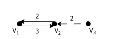
Figure 9. The labelled graph $(\mathcal{G},\ell)$ with orientation $E_{\theta}$.

Then any multiple of $6$ is admissible. For example for $q=6$ we denote the $6$-flows as vectors of $(\mathbb{Z}/6\mathbb{Z})^{3}$, where for every $i=1,2,3$, the $i$-th coordinate corresponds to the weight of the edge $e_{i}$.

In this case there are $4$ possible $6$-flows of $(\mathcal{G},\ell)$: $(\overline{3},\overline{2},\overline{0})$, $(\overline{3},\overline{2},\overline{3})$, $(\overline{3},\overline{4},\overline{0})$, $(\overline{3},\overline{4},\overline{3})$.

We define the arithmetic flow polynomial of a labelled graph $(\mathcal{G},\ell)$ to be the function ${\chi}_{\mathcal{G},\ell}^{*}(\cdot):\mathbb{N}\setminus\{0\}\rightarrow\mathbb{N}\cup\{0\}$, which assign to each positive integer $q$ the number of arithmetic $q$-flows of $(\mathcal{G},\ell)$. We will show in Theorem 5.2 that this is in fact a polynomial function.

Remark 5.2.

For a trivial labelling $\ell\equiv 1$ and $D=\emptyset$, clearly we just recover the usual notion of flow polynomial ${\chi}_{\mathcal{G}}^{*}(q)$ of the underlying graph $\mathcal{G}$.

Example 5.2.

Consider $(\mathcal{G},\ell)$ as in Example 5.1. For the vertex $v_{3}$ we have the equation $2w(e_{3})=0\in H$, for which we have only the two solutions $\overline{0}$ and $\overline{q/2}$. In both cases they don’t contribute the the conditions on the other two vertices. Therefore, for both vertices $v_{1}$ and $v_{2}$ we get the equation $2w(e_{1})-3w(e_{2})=0\in H$, which has $q$ solutions: for every value of $w(e_{2})$ of the form $w(e_{2})=2\overline{a}\in H$ there are exactly two values of $w(e_{1})$ which give a solution, while for the other values of $w(e_{2})$ there are no solutions.

But the inequalities $w(e_{1})\neq 0\in H$ and $w(e_{2})\neq 0\in H$ exclude the four possibilities $(\overline{0},\overline{0})$, $(\overline{0},\overline{q/3})$, $(\overline{0},\overline{2q/3})$, $(\overline{q/2},\overline{0})$ for $(w(e_{1}),w(e_{2}))$. Hence we have $q-4$ solutions.

In conclusion, $\chi_{\mathcal{G},\ell}^{*}(q)=2(q-4)=2q-8$, which agrees with what we found for $q=6$ ($\chi_{\mathcal{G},\ell}^{*}(6)=4$).

Lemma 5.1.

${\chi}_{\mathcal{G,\ell}}^{*}(q)$ does not depend on the orientation that we choose.

Proof.

If we change the orientation of one edge then we can always change the sign of the corresponding weight (which is an element of $H$). ∎

5.2. Main result

We state the main result of this section.

Theorem 5.2.

Given a labelled graph $(\mathcal{G},\ell)$ with $k$ connected components and an admissible integer $q$,

$${\chi}_{\mathcal{G},\ell}^{*}(q)=\widetilde{\chi}_{\mathcal{G},\ell}^{*}(q):=(-1)^{|R|-|\overline{V}|+k}q^{|D|-|V|+|\overline{V}|}M_{\mathcal{G},\ell}(0,1-q).$$

Example 5.3.

Consider $(\mathcal{G},\ell)$ with the orientation as in Example 5.1.

Hence $X_{D}=\left\{(0,2,-2)\right\}$ $\subseteq\mathbb{Z}^{3}$ and $X_{R}\equiv\left\{\overline{(2,-2,0)},\overline{(-3,3,0)}\right\}\subseteq G:=\mathbb{Z}^{3}/\langle X_{D}\rangle=\mathbb{Z}^{3}/\langle(0,2,-2)\rangle$. An easy computation shows that $M_{\mathcal{G},\ell}(x,y)=2x+6+2y$, and therefore

$$\widetilde{\chi}_{\mathcal{G},\ell}^{*}(q)=-M_{\mathcal{G},\ell}(0,1-q)=2q-8=\chi_{\mathcal{G},\ell}^{*}(q),$$

as predicted.

Remark 5.3.

The admissibility condition on $q$ (i.e. $\ell(e)$ divides it for all $e\in E$) is necessary: for example, consider $(\mathcal{G},\ell)$, where $\mathcal{G}:=(V,E)$ with $V:=\{v_{1},v_{2},v_{3}\}$, $R:=\emptyset$, $D:=\{\{v_{1},v_{2}\},\{v_{2},v_{3}\}\}$ so that $E=R\cup D$, and $\ell(\{v_{1},v_{2}\})=2$, $\ell(\{v_{2},v_{3}\})=6$.

For $q=2$, the conditions on the flows are trivially satisfied, hence we have $2^{2}=4$ $2$-flows.

Recall from Remark 3.3 the associated arithmetic matroid for the fixed orientation $E_{\theta}=\{(v_{1},v_{2})$, $(v_{3},v_{2})\}$ (see Figure 10).

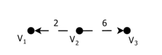
Figure 10. The labelled graph $(\mathcal{G},\ell)$ with orientation $E_{\theta}$.

We computed $M_{\mathcal{G},\ell}(x,y)=12$, therefore

$$\widetilde{\chi}_{\mathcal{G},\ell}^{*}(q)=M_{\mathcal{G},\ell}(0,1-q)=12.$$

But then

$$\widetilde{\chi}_{\mathcal{G},\ell}^{*}(2)=12\neq 4=\chi_{\mathcal{G},\ell}^{*}(2).$$

If $|D|=\emptyset$ and $\ell\equiv 1$, then we can identify the graph $\mathcal{G}$ with $\overline{\mathcal{G}}$ (cf. Remark 5.2). In this case all the multiplicities in $\mathfrak{M}_{\mathcal{G},\ell}$ are equal to $1$, therefore we recover the following classical result of Tutte [7] (cf. also [8, Proposition 6.3.4]) as a special case of Theorem 5.2.

Corollary 5.3.

We have

$${\chi}_{\mathcal{G}}^{*}(q)=(-1)^{|E|-|V|+k}T_{\mathcal{G}}(0,1-q),$$

where ${\chi}_{\mathcal{G}}^{*}(q)$ is the flow polynomial of the graph $\mathcal{G}=(V,E)$, $k$ is the number of connected components of $\mathcal{G}$ and $T_{\mathcal{G}}(x,y)$ is the associated Tutte polynomial.

6. Proof of Theorem 5.2

To prove Theorem 5.2 we need the following lemma.

Lemma 6.1.

Let $(\mathcal{G},\ell)$ be a labelled graph and let $q$ be an admissible integer. For a regular edge $e\in R$ we have

$${\chi}_{\mathcal{G,\ell}}^{*}(q)={\chi}_{\mathcal{G}/e,\ell}^{*}(q)-{\chi}_{\mathcal{G}-e,\ell}^{*}(q).$$

Proof.

It is enough to observe that the deletion of $e$ corresponds to impose the equation $w(e)=0\in H$. Then the result is clear from the definitions. ∎

We want to prove that our polynomial $\widetilde{{\chi}}_{\mathcal{G},\ell}^{*}(q)$ satisfies the same recursion.

Lemma 6.2.

Let $(\mathcal{G},\ell)$ be a labelled graph and let $q$ be an admissible integer. For a regular edge $e\in R$ we have

$$\widetilde{\chi}_{\mathcal{G,\ell}}^{*}(q)=\widetilde{\chi}_{\mathcal{G}/e,\ell}^{*}(q)-\widetilde{\chi}_{\mathcal{G}-e,\ell}^{*}(q).$$

Proof.

We distinguish three cases.

Case 1: $e$ is a proper edge, i.e. the corresponding edge in $\overline{\mathcal{G}}$ is not a loop and it is contained in a circuit. Then, applying Theorem 2.1 (1), we have

$$\widetilde{\chi}_{\mathcal{G,\ell}}^{*}(q) = (-1)^{|R|-|\overline{V}|+k}q^{|D|-|V|+|\overline{V}|}M_{X_{R}}(0,1-q)$$

$$= (-1)^{|R|-|\overline{V}|+k}q^{|D|-|V|+|\overline{V}|}(M_{X_{R_{2}}}(0,1-q)+M_{X_{R_{1}}}(0,1-q))$$

$$= (-1)^{|R_{2}|-|\overline{V}_{2}|+k}q^{|D_{2}|-|V|+|\overline{V}_{2}|}M_{X_{R_{2}}}(0,1-q)$$

$$- (-1)^{|R_{1}|-|\overline{V}_{1}|+k}q^{|D_{1}|-|V|+|\overline{V}_{1}|}M_{X_{R_{1}}}(0,1-q)$$

$$= \widetilde{\chi}_{\mathcal{G}/e,\ell}^{*}(q)-\widetilde{\chi}_{\mathcal{G}-e,\ell}^{*}(q),$$

since $|R_{1}|=|R_{2}|=|R|-1$, $|D_{1}|=|D|$, $|D_{2}|=|D|+1$, $|\overline{V}_{1}|=|\overline{V}|$ and $|\overline{V}_{2}|=|\overline{V}|-1$.

Case 2: $e$ is a free edge, i.e. the corresponding edge in $\overline{\mathcal{G}}$ is not contained in a circuit and is not a loop. Then, applying Theorem 2.1 (2), we have

$$\widetilde{\chi}_{\mathcal{G,\ell}}^{*}(q) = (-1)^{|R|-|\overline{V}|+k}q^{|D|-|V|+|\overline{V}|}M_{X_{R}}(0,1-q)$$

$$= (-1)^{|R|-|\overline{V}|+k}q^{|D|-|V|+|\overline{V}|}(M_{X_{R_{2}}}(0,1-q)-M_{X_{R_{1}}}(0,1-q))$$

$$= (-1)^{|R_{2}|-|\overline{V}_{2}|+k}q^{|D_{2}|-|V|+|\overline{V}_{2}|}M_{X_{R_{2}}}(0,1-q)$$

$$- (-1)^{|R_{1}|-|\overline{V}_{1}|+(k+1)}q^{|D_{1}|-|V|+|\overline{V}_{1}|}M_{X_{R_{1}}}(0,1-q)$$

$$= \widetilde{\chi}_{\mathcal{G}/e,\ell}^{*}(q)-\widetilde{\chi}_{\mathcal{G}-e,\ell}^{*}(q),$$

since $\mathcal{G}-e$ has now an extra connected component, $|D_{1}|=|D|$, $|D_{2}|=|D|+1$, $|R_{1}|=|R_{2}|=|R|-1$, $|\overline{V}_{1}|=|\overline{V}|$ and $|\overline{V}_{2}|=|\overline{V}|-1$.

Case 3: $e$ is a torsion edge, i.e. the corresponding edge in $\overline{\mathcal{G}}$ is a loop. Then, applying Theorem 2.1 (3), we have

$$\widetilde{\chi}_{\mathcal{G,\ell}}^{*}(q) = (-1)^{|R|-|\overline{V}|+k}q^{|D|-|V|+|\overline{V}|}M_{X_{R}}(0,1-q)$$

$$= (-1)^{|R|-|\overline{V}|+k}q^{|D|-|V|+|\overline{V}|}(-qM_{X_{R_{2}}}(0,1-q)+M_{X_{R_{1}}}(0,1-q))$$

$$= (-1)^{|R_{2}|-|\overline{V}_{2}|+k}q^{|D_{2}|-|V|+|\overline{V}_{2}|}M_{X_{R_{2}}}(0,1-q)$$

$$- (-1)^{|R_{1}|-|\overline{V}_{1}|+k}q^{|D_{1}|-|V|+|\overline{V}_{1}|}M_{X_{R_{1}}}(0,1-q)$$

$$= \widetilde{\chi}_{\mathcal{G}/e,\ell}^{*}(q)-\widetilde{\chi}_{\mathcal{G}-e,\ell}^{*}(q),$$

since $|D_{1}|=|D|$, $|D_{2}|=|D|+1$, $|R_{1}|=|R_{2}|=|R|-1$, $|\overline{V}_{1}|=|\overline{V}|$ and $|\overline{V}_{2}|=|\overline{V}|$. ∎

In this way we reduce the proof of Theorem 5.2 to the case where there are no regular edges. For this case, first of all we reduce ourself to the case of a connected graph: suppose that our graph $\mathcal{G}$ has $k$ connected components $\mathcal{G}^{(1)},\mathcal{G}^{(2)},\dots,\mathcal{G}^{(k)}$ with the corresponding labellings $\ell^{(1)},\ell^{(2)},\dots,\ell^{(k)}$. In this case the matroid $\mathfrak{M}_{\mathcal{G},\ell}$ is the direct sum of the matroids $\mathfrak{M}_{\mathcal{G}^{(1)},\ell^{(1)}},\mathfrak{M}_{\mathcal{G}^{(2)},\ell^{(2)}},\dots,\mathfrak{M}_{\mathcal{G}^{(k)},\ell^{(k)}}$ (cf. Remark 2.2). Since $\overline{\mathcal{G}^{(i)}}$ consists of a single vertex with no edges for $i=1,2,\dots,k$, we have $|\overline{V}|=k$. We denote by $D^{(i)}$ and $V^{(i)}$ the set of dotted edges and vertices respectively of $\mathcal{G}^{(i)}$. Therefore, assuming the result for a connected graph, we have

$$(-1)^{|R|-|\overline{V}|+k}q^{|D|-|V|+|\overline{V}|}M_{\mathcal{G},\ell}(0,1-q) = q^{|D|-|V|+k}M_{\mathcal{G},\ell}(0,1-q)$$

(by Theorem 2.1 (4)) $$= q^{|D|-|V|+k}\cdot\prod_{i=1}^{k}M_{\mathcal{G}^{(i)},\ell^{(i)}}(0,1-q)$$

$$= \prod_{i=1}^{k}q^{|D^{(i)}|-|V^{(i)}|+1}M_{\mathcal{G}^{(i)},\ell^{(i)}}(0,1-q)$$

(by assumption on connected graphs) $$= \prod_{i=1}^{k}{\chi}_{\mathcal{G}^{(i)},\ell^{(i)}}^{*}(q)={\chi}_{\mathcal{G},\ell}^{*}(q),$$

where the last equality is clear from the definition of arithmetic flow polynomial.

So we are left to prove the following lemma.

Lemma 6.3.

Let $(\mathcal{G},\ell)$ be a labelled connected graph with no regular edges and let $q$ be an admissible integer. We have

$${\chi}_{\mathcal{G},\ell}^{*}(q)=\widetilde{{\chi}}_{\mathcal{G},\ell}^{*}(q).$$

Proof.

First of all, if we set $m:=|E|=|D|$ and $n:=|V|$, notice that

$$\widetilde{{\chi}}_{\mathcal{G},\ell}^{*}(q)=q^{m-n+1}\cdot M_{\mathcal{G},\ell}(0,1-q)=q^{m-n+1}\cdot m(\emptyset),$$

where $m(\emptyset)$ is the cardinality of the torsion subgroup of the group $\mathbb{Z}^{n}/\langle X_{D}\rangle$, i.e. the GCD of the maximal rank nonzero minors of the matrix $[X_{D}]$ whose columns are the elements of $X_{D}$ (cf. Remark 2.1).

To compute the number of arithmetic $q$-flows, observe that $m=|X_{D}|$, and $m\geq n-1$ (we are assuming that $\mathcal{G}$ is connected). We can look at $[X_{D}]$ as a linear operator (acting on the left)

$$[X_{D}]:(\mathbb{Z}/q\mathbb{Z})^{m}\rightarrow(\mathbb{Z}/q\mathbb{Z})^{n}.$$

Then the elements of the kernel correspond naturally to the arithmetic $q$-flows, hence we need to compute the cardinality of $Ker[X_{D}]$. Looking at the exact sequence (i.e. the image of each homomorphism is the kernel of the successive one)

$$0\rightarrow Ker[X_{D}]\mathop{\hookrightarrow}^{\iota}(\mathbb{Z}/q\mathbb{Z})^{m}\mathop{\longrightarrow}^{[X_{D}]}(\mathbb{Z}/q\mathbb{Z})^{n}\mathop{\longrightarrow}^{\pi}\frac{(\mathbb{Z}/q\mathbb{Z})^{n}}{Im[X_{D}]}\rightarrow 0,$$

where $\iota$ and $\pi$ are the inclusion and the natural map to the quotient respectively, we realize that $(\mathbb{Z}/q\mathbb{Z})^{m}/Ker[X_{D}]\cong Im[X_{D}]$ implies

$$\frac{|(\mathbb{Z}/q\mathbb{Z})^{n}|}{|Im[X_{D}]|}=\frac{|(\mathbb{Z}/q\mathbb{Z})^{n}|}{|(\mathbb{Z}/q\mathbb{Z})^{m}|}\cdot|Ker[X_{D}]|=q^{n-m}\cdot|Ker[X_{D}]|.$$

Now by the isomorphism theorem

$$|(\mathbb{Z}/q\mathbb{Z})^{n}:Im[X_{D}]|=|\mathbb{Z}^{n}:Im[X_{D}\cup Q]|,$$

where $Q=\{q_{1},q_{2},\dots,q_{n}\}$, $q_{i}$ is the vector of $\mathbb{Z}^{n}$ with $1$ in the $i$-th position and $0$ elsewhere, and we see the matrix $[X_{D}\cup Q]$ (whose columns are the elements of $X_{D}$ and of $Q$) as a linear operator (acting on the left)

$$[X_{D}\cup Q]:\mathbb{Z}^{n+m}\rightarrow\mathbb{Z}^{n}.$$

But when we compute the right-hand side of the last equation we get $q\cdot m(\emptyset)$. In fact by Remark 2.1 this the $GCD$ of the minors of maximal rank of $[X_{D}\cup Q]$. But, since $\ell(e)$ divides $q$ for every edge $e\in E$ ($=D$ in this case), it is enough to compute the minors of maximal rank which involve the edges of a spanning tree plus an extra columns from $Q$ (the other ones are multiples of these). Therefore we get $q$ times the $GCD$ of minors of rank $n-1$ in $[X_{D}]$, which are the ones corresponding to spanning trees. But this last number is exactly $m(\emptyset)$.

From all this we get

$$\chi_{\mathcal{G},\ell}^{*}(q)=|Ker([X_{D}])|=q^{m-n+1}\cdot m(\emptyset)=q^{m-n+1}\cdot M_{\mathcal{G},\ell}(0,1-q)=\widetilde{\chi}_{\mathcal{G},\ell}^{*}(q),$$

as we wanted. ∎

7. Final comments

Recall that the dual of a matroid $\mathfrak{M}_{X}=(X,rk)$ is the matroid $\mathfrak{M}_{X}^{*}=(X,rk^{*})$ on $X$ whose rank function $rk^{*}$ is given by the formula

$$rk^{*}(A):=|X|-rk(X)+rk(X\setminus A)$$

for all $A\subseteq X$.

If we denote by $T(\mathfrak{M}_{X};x,y)$ and $T(\mathfrak{M}_{X}^{*};x,y)$ the Tutte polynomial of $\mathfrak{M}_{X}$ and $\mathfrak{M}_{X}^{*}$ respectively, then we have the easy relation

$$T(\mathfrak{M}_{X}^{*};x,y)=T(\mathfrak{M}_{X};y,x).$$

Consider a graph $\mathcal{G}$ whose associated matroid is $\mathfrak{M}_{\mathcal{G}}$ and suppose now that the dual matroid $\mathfrak{M}_{\mathcal{G}}^{*}$ is realized by another graph $\mathcal{G}^{*}$. In this case $\mathcal{G}^{*}$ is called a dual graph of $\mathcal{G}$.

It turns out that the graphs $\mathcal{G}$ that admit such a dual are exactly the planar graphs, for which a dual graph is still planar and it can be constructed explicitly starting from the graph and its planar embedding (see [4, Section 1.8]).

These remarks together with Corollaries 3.2 and 5.3 suggest that there should be a sort of duality between the colorings of $\mathcal{G}$ and the flows of $\mathcal{G}^{*}$.

Similarly, the dual of an arithmetic matroid $(\mathfrak{M}_{X},m)$ is simply the arithmetic matroid $(\mathfrak{M}_{X}^{*},m^{*})$, where $m^{*}(A):=m(X\setminus A)$ for all $A\subseteq X$ (see [2] for the proofs of the statements in this discussion).

If we denote by $M(\mathfrak{M}_{X};x,y)$ and $M(\mathfrak{M}_{X}^{*};x,y)$ the arithmetic Tutte polynomial of $(\mathfrak{M}_{X},m)$ and $(\mathfrak{M}_{X}^{*},m^{*})$ respectively, then we have the easy relation

$$M(\mathfrak{M}_{X}^{*};x,y)=M(\mathfrak{M}_{X};y,x).$$

Consider a labelled graph $(\mathcal{G},\ell)$ whose associated arithmetic matroid is $\mathfrak{M}_{\mathcal{G},\ell}$ and suppose now that the dual matroid $\mathfrak{M}_{\mathcal{G},\ell}^{*}$ is realized by another labelled graph $(\mathcal{G}^{*},\ell^{*})$, which we call a dual of $(\mathcal{G},\ell)$.

These remarks together with Theorems 3.1 and 5.2 suggest that there should be a sort of duality between the arithmetic colorings of $(\mathcal{G},\ell)$ and the arithmetic flows of $(\mathcal{G}^{*},\ell^{*})$.

It is now natural to formulate the following vague problem, that we leave open.

Problem.

Find a topological-arithmetic characterization (and eventually an explicit construction) of the dual of a labelled graph.

We finally remark that for passing from the labelled graph to its arithmetic matroid we went through a list of elements in a finitely generated abelian group. For these in [2] we proved (giving an explicit construction) that the dual matroid arise again from such a list.

References

- [1] M. D’Adderio, L. Moci, Ehrhart polynomial of the zonotope and multiplicity Tutte polynomial, arXiv:1102.0135 [math.CO].
- [2] M. D’Adderio, L. Moci, Arithmetic matroids, Tutte polynomial and toric arrangements, arXiv:1105.3220v2 [math.CO].
- [3] C. De Concini, C. Procesi, Topics in hyperplane arrangements, polytopes and box-splines, Universitext, Springer-Verlag, New-York (2010), XXII+381 pp.
- [4] C. Godsil, G. Royle, Algebraic graph theory, GTM, Springer-Verlag, New-York (2000), XX+439 pp.
- [5] L. Moci, A Tutte polynomial for toric arrangements, arXiv:0911.4823v4 [math.CO], to appear on Trans. Am. Math. Soc.
- [6] R. P. Stanley, A zonotope associated with graphical degree sequences, in Applied Geometry and Discrete Combinatorics, DIMACS Series in Discrete Mathematics, vol. 4, 1991, pp. 555-570.
- [7] W. T. Tutte, A contribution to the theory of chromatic polynomials, Canadian J. Math., 6: 80-91, 1954
- [8] N. White, Matroid Applications, Encyclopedia of Mathematics and Its Applicaitons, vol. 40, Cambridge University Press, (1992).