Robustness of a Tree-like Network of Interdependent Networks (28 August)

Abstract

In reality, many real-world networks interact with and depend on other networks. We develop an analytical framework for studying interacting networks and present an exact percolation law for a network of $n$ interdependent networks (NON). We present a general framework to study the dynamics of the cascading failures process at each step caused by an initial failure occurring in the NON system. We study and compare both $n$ coupled Erdős-Rényi (ER) graphs and $n$ coupled random regular (RR) graphs. We found recently [Gao et. al. arXive:1010.5829] that for an NON composed of $n$ ER networks each of average degree $k$, the giant component, $P_{\infty}$, is given by $P_{\infty}=p[1-\exp(-kP_{\infty})]^{n}$ where $1-p$ is the initial fraction of removed nodes. Our general result coincides for $n=1$ with the known Erdős-Rényi second-order phase transition at a threshold, $p=p_{c}$, for a single network. For $n=2$ the general result for $P_{\infty}$ corresponds to the $n=2$ result [Buldyrev et. al., Nature , 464, (2010)]. Here we show for an NON composed of $n$ coupled RR networks each of degree $k$, that the giant components is given by $P_{\infty}=p\big{\{}1-\{p^{1/n}P_{\infty}^{(n-1)/n}[(1-(P_{\infty}/p)^{1/n})^{(k-1)/k}-1]+1\}^{k}\big{\}}^{n}$. Similar to the ER NON, for $n=1$ the percolation transition at $p_{c}$, is of second order while for any $n>1$ it is of first order. The first order percolation transition in both ER and RR (for $n>1$) is accompanied by cascading failures between the networks due to their interdependencies. However, we find that the robustness of $n$ coupled RR networks of degree $k$ is dramatically higher compared to the $n$ coupled ER networks of average degree $k$. While for ER NON there exists a critical minimum average degree $k=k_{\min}$, that increases with $n$, below which the system collapses, there is no such analogous $k_{\min}$ for RR NON system. For any $k>2$, the RR NON is stable, i.e., $p_{c}<1$. This is due to the critical role played by singly connected nodes which exist in ER NON and enhance the cascading failures but do not exist in the RR NON system.

I Introduction

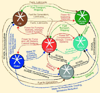
In our modern world, infrastructures, which affect all areas of daily life, are usually interdependent. Examples include, electric power, natural gas and petroleum production and distribution, telecommunications, transportation, water supply, banking and finance, emergency and government services, agriculture, and other fundamental systems and services that are critical to the security, economic prosperity, and social systems, shown in Fig.1. Although urban societies rely on each of the individual infrastructures, recent disasters ranging from hurricanes to large-scale power blackout and terrorist attacks have shown that significant dangerous vulnerability is due to the many interdependencies across different infrastructures Chang2009 ; Rinaldi2001 ; Alessandro2010 ; John2008 ; Rosato2008 . Infrastructures are frequently connected at multiple points through a wide variety of mechanisms, such that a bidirectional relationship exists between the states of any given pair of networks, as shown in Fig. 1 and 2 Rinaldi2001 . For example, in California, electric power disruptions in early 2001 affected oil and natural gas production, refinery operations, pipeline transport of gasoline and jet fuel within California and its neighboring states, and the movement of water from northern to central and southern regions of the state for crop irrigation. Another dramatic real-world example of a cascade of failures is the electrical blackout that affected much of Italy on 28 September 2003: the shutdown of power stations directly led to the failure of nodes in the Supervisory Control and Data Acquisition (SCADA) communication network, which in turn caused further breakdown of power stations Rosato2008 ; Sergey2010 . Identifying, understanding, and analyzing such interdependencies are significant challenges. These challenges are greatly magnified by the breadth and complexity of our modern critical national interdependent infrastructures John2008 .

In recent years we observed important advances in the field of complex networks  Strogatz1998 ; bara2000 ; Callaway2000 ; Albert2002 ; Cohen2000 ; Newman2003 ; Dorogovtsev2003 ; song2005 ; Pastor2006 ; Caldarelli2007 ; Barrat2008 ; Shlomo2010 ; Neman2010 . The internet, airline routes, and electric power grids are all examples of networks whose function relies crucially on the connectivity between the network components. An important property of such systems is their robustness to node failures. Almost all research has been concentrated on the case of a single or isolated network which does not interact with or depend on other networks. Recently, based on the motivation that modern infrastructures are becoming significantly more dependent on each other, a system of two coupled interdependent networks has been studied Sergey2010 ; parshani2010 ; Wei2011 . A fundamental property of interdependent networks is that when nodes in one network fail, they may lead to the failure of dependent nodes in other networks which may cause further damage in the first network and so on, leading to a global cascade of failures. Buldyrev et al. Sergey2010 developed a framework for analyzing the robustness of two interacting networks subject to such cascading failures. They found that interdependent networks behave very different from single networks and become significantly more vulnerable compared to their noninteracting counterparts.

In many realistic examples, more than two networks depend on each other. For example, diverse infrastructures, such as water and food supply, communications, fuel, financial transactions, and power stations are coupled together Peerenboom2001 ; Rinaldi2001 ; Rosato2008 ; Alessandro2010 . Understanding the vulnerability due to such interdependencies is a major challenges for designing resilient infrastructures.

Figure 1: Illustration of the interdependent relationship among different infrastructures Rinaldi2001 . These complex relationships are characterized by multiple connections between infrastructures, feedback and feedforward paths, and intricate, branching topologies. The connections create an intricate web that, depending on the characteristics of its linkages, can transmit shocks throughout broad swaths of an economy and across multiple infrastructures. It is clearly impossible to adequately analyze or understand the behavior of a given infrastructure in isolation from the environment or other infrastructures. Rather, one must consider multiple interconnected infrastructures and their interdependencies. For example, the reliable operation of modern infrastructures depends on computerized control systems, from SCADA systems that control electric power grids to computerized systems that manage the flow of railcars and goods in the rail industry. In these cases, the infrastructures require information transmitted and delivered by the communication infrastructure Rinaldi2001 .

We study here a model system  gao2010 , comprising a network of $n$ coupled networks, where each network consists of $N$ nodes (See Fig. 2). The $N$ nodes in each network are connected to nodes in neighboring networks by bidirectional dependency links, thereby establishing a one-to-one correspondence. We apply a mathematical framework gao2010 to study the robustness of tree-like “network of networks” (NON) by studying the dynamically process of the cascading failures. We find an exact analytical law for percolation of a NON system composed of $n$ coupled randomly connected networks. Our result generalizes the known Erdős-Rényi (ER) ER1959 ; ER1960 ; Bollob1985 result as well as the random regular (RR) result for the giant component of a single network, and shows that while for $n=1$ the percolation transition is a second order, for $n>1$ cascading failures occur and the transition becomes a first order transition. Our results for $n$ interdependent networks show that the classical percolation theory extensively studied in physics and mathematics is in fact a limited case of the rich, general, and very different percolation law which exists in realistic interacting networks.

Additionally, we find:

(i) for any loopless topology of NON, the critical percolation threshold and the giant component depend only on the number of networks involved and their degree distributions but not on the inter-linked topology (Fig. 2),

(ii) the robustness of NON significantly decreases with $n$, and

(iii) for a network of $n$ ER networks all with the same average degree $k$, there exists a minimum degree $k_{\min}(n)$ increasing with $n$, below which $p_{c}=1$, i.e., for $k<k_{\min}$ the NON will collapse once any finite number of nodes fail. The analytical expression for $k_{\min}(n)$ generalizes the known result $k_{\min}(1)=1$ for ER below which the network collapses. In sharp contrast a NON composed of RR networks is significantly more robust. In the RR NON case there is no $k_{\min}$ below which the NON collapses. This is due to the multiple links of each node in the RR system compared to the existence of singely connected nodes in the ER case. We also discuss the critical effect of singly connected nodes on the vulnerability of the NON ER structure.

Figure 2: (color online) Three types of loopless NONs composed of five coupled networks all have same percolation threshold and same giant percolation component.

II The dynamic process of cascading failures

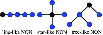
To model an interdependent NON we consider for simplicity and without loss of generality, $n$ networks each having $N$ nodes. We study the percolation of $n$ networks connected in a loopless structure, the structure of the NON can be, e.g., a line, a star or a tree as shown in Fig. 2. Each node in Fig. 2 represents a network, and each link between two networks $i$ and $j$ denotes the existence of a one-to-one dependencies between the nodes of the linked networks. The functioning of one node in network $i$ depends on the functioning of one and only one node in network $j$ ($i,j\in\{1,2,...,n\},i\neq j$), and vice versa (bidirectional links). We assume that within network $i$, the nodes are randomly connected by $A_{i}$-links with degree distribution $P(k_{i})$, where $k_{i}$ is the average degree of network $i$.

The root of the NON is the network from which fraction $1-p$ of nodes are removed due to random failure. Before showing the dynamic of the cascading failures, we present the following three definitions. (i) We define the distance matrix $D_{ij}$ as the distance form network $i$ to network $j$ in the NON. (ii) Shell $j$ is a set $L_{j}$ whose networks are at distance $j$ from the root network, where $j\in[0,s]$ and $s$ is the total number of shells. In the following example, we use $i_{j}$ to denote network $i$ in shell $j$, e.g., ${i_{j}}\in L_{j}$. Note that in shell 0, there is one and only one network $1_{0}$. (iii) $g_{i}(x)$ is the generating function of network $i$ Newman2001 , which reflects the topology of network $i$ and satisfies

$$g_{i}(x)=1-G_{0,i}(x,f_{i}).$$ (1)

where $G_{0,i}(x,f_{i})$ satisfies Newman2001 ; Newman2002PRE ; Sergey2010

$$G_{0,i}(x,f_{i})=G_{0,i}(xf_{i}+1-x)=\sum^{\infty}_{k=0}{P_{i}(k)(xf_{i}+1-x)^{k}},$$ (2)

and

$$G_{1}(x,f)=G^{\prime}_{0}(x,f)/G^{\prime}_{0}(1)=f.$$ (3)

Next, we show analytically the steps in the dynamics of the cascading failures as demonstrated in Fig. 3.

Figure 3: The dynamic of cascading failures. In this figure, each node represents a network. The arrow (on the link) illustrates the damage spreading from the root network to the whole NON shell by shell.

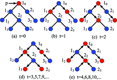
Step (0): At $t=0$ (Fig. 3(a)), we begin by randomly removing a fraction $1-p$ of nodes from the root network (network $1_{0}$), and removing all the $A_{1_{0}}$-links connected to these removed nodes. Next we remove all the nodes that become disconnected to the largest component of network $1_{0}$. Thus at $t=0$, for the network $1_{0}$, the fraction of remaining nodes in network $1_{0}$ after the initial failure is $x_{0,1_{0}}=p$ and the fraction nodes in the giant component $\mu_{0,1_{0}}=pg_{1_{0}}(p)$.

Step (1): At $t=1$, the root network spreads its damages to all its neighboring networks ${i_{1}}\in L_{1}$ (Fig. 3(b)). So we remove all nodes in networks ${i_{1}}$ that are connected to the removed nodes in network $1_{0}$ and then remove all the nodes not in the giant components of networks ${i_{1}}$. At $t=1$, the failure of networks $i_{1}$ is equivalent to a random removal of the fraction of $1-x_{1,i_{1}}$ nodes from networks $i_{1}$ Sergey2010 , where $x_{1,i_{1}}=pg_{1_{0}}(x_{0,1_{0}})$, and the giant component of network $i_{1}$ is $\mu_{1,i_{1}}=x_{1,i_{1}}g_{i_{1}}(x_{1,i_{1}})$.

Step (2): At $t=2$, the networks ${i_{1}}\in L_{1}$ reflects their damages back to the root network and spreads their damages to all their neighboring networks ${j_{2}}\in L_{2}$ (See Fig. 3(c)). So we remove all nodes in networks $1_{0}$ and ${j_{2}}$ that are connected to the removed nodes in networks ${i_{1}}$ and then removing all the nodes not in the giant components of networks ${i_{1}}$. Again the failure of network $1_{0}$ is equivalent to a random removal of the fraction of $1-x_{2,1_{0}}$ nodes from networks $1_{0}$, where $x_{2,1_{0}}=p\prod_{i_{1}\in L_{1}}g_{i_{1}}(x_{1,i_{1}})$; the failure of networks $j_{2}$ is equivalent to a random removal of the fraction of $1-x_{2,j_{2}}$ nodes from networks $j_{2}$, where $x_{2,j_{2}}=pg_{1_{0}}(x_{0,1_{0}})g_{i_{1}}(x_{1,i_{1}})$ for networks $i_{1}$ that are linked to networks $j_{2}$.

Step (3): At $t=3$, the root network spreads its further damages to the networks ${i_{1}}$ in shell 1 again, the networks ${j_{2}}$ in shell 2 reflect their damages back to the neighboring networks ${i_{1}}$ in shell 1, and to the neighboring networks ${u_{3}}$ in shell 3 as shown in Fig. 3(d). A network in ${i_{1}}$ receives the damages information $x_{2,1_{0}}$ from network $1_{0}$, $x_{2,i_{2}}$ from networks ${j_{2}}$ that are linked to networks $i_{1}$, and $x_{1,v_{1}}$ from networks ${v_{1}}$ in shell 1 where the networks $v_{1}$ are the neighboring networks of $i_{1}$’s neighboring networks, i.e., the distance between networks $i_{1}$ and networks $v_{1}$ is 2. Thus we can obtain that $x_{3,i_{1}}=pg_{1_{0}}(x_{2,1_{0}})\prod_{j_{2}}g_{j_{2}}(x_{2,j_{2}})\prod_{v_{1}}g_{v_{1}}(x_{1,v_{1}})$. Similarly, we obtain the failure of networks ${u_{3}}\in L_{3}$ to be $x_{3,u_{3}}=pg_{1_{0}}(x_{0,1_{0}})g_{i_{1}}(x_{1,i_{1}})g_{j_{2}}(x_{2,j_{2}})$, where networks ${u_{3}}$ in shell 3 are connected to networks ${j_{2}}$ in shell 2 and networks ${j_{2}}$ are connected to networks ${i_{1}}$ in shell 1.

Figure 4: How does the damage spread in a NON system? In this figure, each node represents a network. When looking at network 12 for example, it becomes damaged at $t=2k+1$ ($k=1,2,3,...$). It receives the damage from network 8 at $t=2k+3$, because network 8 gets damage at $t=2$ for the first time and its damage spreads to network 12 when $t=5$ for the first time, which agrees with Eqs. (4-8) that network $i$ receives damage from network $j$ if and only if $t-D_{ij}\geq D_{1j}$.

We continue the cascading process step by step [see Figs. 3(d) and (e)] until the convergence step, $t=\tau$, when no further nodes and links removal occurs. Accordingly, we investigate the dynamically cascading process of our model of the loopless NON. First we initialize the NON as

$$x_{0,1_{0}}=p,\mu_{0,1}=pg_{1_{0}}(p),$$ (4)

and

$$g_{i_{j}}(x_{t,i_{j}})=\mu_{t,i_{j}}=1,t<j.$$ (5)

Thus we can obtain that the giant component of network $i_{j}$ in shell $j$, $\mu_{t,i_{j}}$ at step $t$ satisfies

$$\mu_{t,i_{j}}=x_{t,i_{j}}g_{i_{j}}(x_{t,i_{j}}),j\in C(t),$$ (6)

$$\mu_{t,i_{j}}=\mu_{t-1,i_{j}},j\notin C(t).$$ (7)

where $C(t)$ satisfies the sequence

$\left\{\begin{array}[]{lcl}C(0)=\{0\}&\mbox{}&\\ C(1)=\{1\}&\mbox{}&\\ C(2)=\{0,2\}&\mbox{}&\\ C(3)=\{1,3\}&\mbox{}&\\ C(4)=\{0,2,4\}&\mbox{}&\\ C(5)=\{1,3,5\}&\mbox{}&\\ C(6)=\{0,2,4,6\}&\mbox{}&\\ C(7)=\{1,3,5,7\}&\mbox{}&\\ C(8)=\{0,2,4,6,8\}&\mbox{}&\\ ...&\mbox{}&\\ \end{array}\right.$,

and $x_{t,i}$ satisfies

$$x_{t,i}=p\prod_{j=1,j\neq i}^{n}g_{j}(x_{t-D_{ij},i}).$$ (8)

Furthermore, when $t\longrightarrow\infty$, $\mu_{i}\equiv\mu_{\infty}$ and $x_{t-D_{ij},i}=x_{t,i}\equiv x_{i}$. So from Eqs. (4-8) we can obtain that

$$x_{i}=p\prod_{j=1,j\neq i}^{n}g_{j}(x_{j}),$$ (9)

and

$$\mu_{\infty}=p\prod_{j=1}^{n}g_{j}(x_{j}).$$ (10)

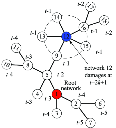
We also demonstrate how does the damage spread in another example of NON shown in Fig. 4.

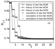
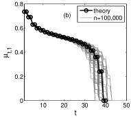
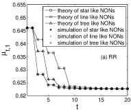
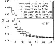
In Figs. 5 and 6 we compare our theoretical results Eqs. (9) and (10) with simulation results for 3 different types of networks, ER networks, RR networks and SF networks. We find that while the dynamics is different for the three topologies shown in Fig. 2, the final $P_{\infty}\equiv\mu_{\infty,1}$ is the same as predicted by the theoretical results, Eq. (27).

Next, we study the case for $n$ coupled networks where all networks are with the same degree distribution specified by the generating functions $G_{0}(x,f)$ (Eq. (2)) and $G_{1}(x,f)$ (Eq. 3)). By substituting Eq. (1) and (2) into the Eq. (9) and introducing the parameter $z=xf+1-x$, we obtain

$$x=p(1-G_{0}(z))^{n-1}$$ (11)

From Eqs. (3), (11) and (10), the equations for mutual giant component become

$$\frac{1}{p}=\frac{(1-G_{0}(z))^{n-1}(1-G_{1}(z))}{1-z},$$ (12)

and

$$P_{\infty}=p(1-G_{0}(z))^{n}=\frac{(1-G_{0}(z))(1-z)}{1-G_{1}(z)}.$$ (13)

Figure 5: (a) Simulation results of the giant component of the root network $\mu_{t,1}$ after $t$ cascading failures for three types of NON composed of 5 ER networks shown in Fig. 2. For each network in the NON, $N=100,000$ and $k=5$. The value of $p$ chosen is $p=0.85$, and the predicated threshold $p_{c}=0.76449$ (from Eqs. (22) and (24)). All points are the results of averaging over 40 realizations. Note that while the dynamics is different for the three topologies, the final $P_{\infty}\equiv\mu_{\infty,1}$ is the same, i.e., the final $P_{\infty}$ does not depend on the topology of the NON. (b) Simulations of the giant component, $\mu_{t,1}$, for the tree-like NON [Fig. 2] with the same parameters as in (a) but for $p=0.755<p_{c}=0.76449$. The figure shows 50 simulated realizations of the giant component left after $t$ stages of the cascading failures compared with the theoretical prediction of Eqs. (4)-(8).

Figure 6: (a) Simulation results for the giant component of the root network $\mu_{t,1}$ after $t$ cascading failures for three types of NON composed of 5 RR networks. The structures of the NON are as shown in Fig. 2. For each network in the NON, $N=100,000$ and $k=5$ . The value of $p$ chosen is $p=0.65$, and the predicated threshold $p_{c}=0.6047$ [from Eqs. (41) and (43)]. The points are the results of averaging over 40 realizations. It is seen that while the dynamics is different for the three topologies, the final $P_{\infty}\equiv\mu_{\infty,1}$ is the same, i.e., the final $P_{\infty}$ does not depend on the topology of the NON. (b) Simulation results of the giant component of the root network $\mu_{t,1}$ after $t$ cascading failures for three types of NON composed of 5 SF networks shown in Fig. 2. For each network in the NON, $N=100,000$ and $\lambda=2.3$ . The value of $p$ chosen is $p=0.85$(above $p_{c}$). The points are the results of averaging over 40 realizations. We also can see here that while the dynamics is different for the three topologies, the final $P_{\infty}\equiv\mu_{\infty,1}$ is the same.

III THE CASE of NON COMPOSED OF $n$ ER NETWORKS

The case of NON of $n$ Erdős-Rényi (ER) ER1959 ; ER1960 ; Bollob1985 networks with average degrees $k_{1},k_{2},...k_{i},...,k_{n}$ can be solved explicitly gao2010 . In this case, the generating functions of the $n$ networks are Newman2002PRE .

$$G_{1,i}(x)=G_{0,i}(x)=\exp[k_{i}(x-1)].$$ (14)

Accordingly, we obtain that the generating function $g_{i}(x_{i})$ satisfies

$$g_{i}(x_{i})=1-\exp[k_{i}x_{i}(f_{i}-1)],$$ (15)

where $f_{i}=\exp[k_{i}x_{i}(f_{i}-1)]$ and thus $g_{i}(x_{i})=1-f_{i}$. Using Eq. (9) for $x_{i}$ we get

$$f_{i}=\exp[-pk_{i}\prod_{j=1}^{n}(1-f_{j})],i=1,2,...,n.$$ (16)

By introducing a new variable $r=f_{i}^{1/k_{i}},i=1,2,...,n$ into Eq. (16), we can reduce the $n$ equations to a single equation,

$$r=\exp[-p\prod\limits_{i=1}^{n}(1-r^{k_{i}})],$$ (17)

which can be solved graphically for any $p$. For small $p$, Eq. (17) has only the trivial solution $r=1$. This case corresponds to the absence of the mutual giant component and hence to the complete fragmentation of the networks. As $p$ increases a nontrivial solution $r<1$ emerges at some critical value of $p=p_{c}$. The critical case corresponds to the tangential condition:

$$1=\frac{d}{dr}\exp[-p\prod\limits_{i=1}^{n}(1-r^{k_{i}})].$$ (18)

Thus, the critical value of $r$ satisfies a transcendental equation

$$r=\exp\Big{\{}-\frac{\prod\limits_{i=1}^{n}(1-r^{k_{i}})}{\sum\limits_{i=1}^{n}{[k_{i}r^{k_{i}}\prod\limits_{j=1,j\neq i}^{n}(1-r^{k_{j}})]}}\Big{\}}.$$ (19)

From Eqs. (16) and (18) we can obtain the critical percolation threshold $p_{c}$ and the the value of $\mu_{\infty}$ at $p_{c}$ as

$$p_{c}=\Big{\{}\sum\limits_{i=1}^{n}{\big{[}k_{i}f_{i}\prod\limits_{j=1,j\neq i}^{n}(1-f_{j})\big{]}}\Big{\}}^{-1},$$ (20)

and

$$\mu_{\infty}=p\prod\limits_{i=1}^{n}(1-f_{i}).$$ (21)

If $p<p_{c}$, Eqs. (16) have only the trivial solutions ($f_{i}=1$) and $\mu_{\infty}\equiv 0$. When the $n$ networks have the same average degree $k$, $k_{i}=k$ ($i=1,2,...,n$), we obtain from Eq. (16) that $f_{c}\equiv f_{i}(p_{c})$ satisfies gao2010

$$f_{c}=e^{\frac{f_{c}-1}{nf_{c}}}.$$ (22)

This solution can be expressed in terms of the Lambert function $W(x)$ Lambert1758 ; Corless1996 ,

$$f_{c}=-[nW(-\frac{1}{n}e^{-\frac{1}{n}})]^{-1}.$$ (23)

Once $f_{c}$ is known, we obtain $p_{c}$ and $\mu_{\infty,n}\equiv P_{\infty}$ at $p_{c}$ by substituting $k_{i}=k$ into Eqs. (20) and (21)

$$p_{c}=[nkf_{c}(1-f_{c})^{(n-1)}]^{-1}$$ (24)

and

$$P_{\infty}=\frac{1-f_{c}}{nkf_{c}}.$$ (25)

For $n=1$ we obtain the known results $p_{c}=1/k$ and $P_{\infty}=0$ at $p_{c}$ (representing the second order transition) of Erdős-Rényi ER1959 ; ER1960 ; Bollob1985 . Substituting $n=2$ in Eqs. (24) and (25) one obtains the exact results derived in Sergey2010 . Note that for all $n>1$ we obtain $P_{\infty}>0$ at $p_{c}$ representing a first order nature of the percolation transition. For the behavior of $p_{c}$ [Eq.(24)] for large $n$ see Appendix A.

III.1 The minimum degree $k$ and the giant component $P_{\infty}(p)$

Figure 7: The critical fraction $p_{c}$ for different $k$ and $n$ for (a) ER NON system and (b) RR NON system. The results for ER NON system are obtained by Eqs. (22) and (24), while the results of RR NON system are obtained from the solution of Eqs. (41) and (43). The results are in good agreement with simulations. In the simulations $p_{c}$ was calculated from the number of cascading failures which diverge at $p_{c}$ parshani2011

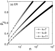
Here we show that while for the ER NON system there exists a minimum degree $k_{\min}(n)$ below which the NON collapses, in the RR NON such a $k_{\min}$ does not exists and the RR NON is stable ($p_{c}(n)<1$) for any $n$. Thus, the RR NON is significantly more robust compared to the ER NON due to the critical role of the singly connected nodes on the vulnerability of the NON system. To analyze $p_{c}$ as a function of $n$, we find $f_{c}$ from Eq. (22) and substitute it into Eq. (24), and we obtain $p_{c}$ as a function of $n$ for different $k$ values, as shown in Fig. 7(a) for the ER NON system. It is seen that the NON becomes more vulnerable with increasing $n$ or decreasing $k$ ($p_{c}$ increases when $n$ increases or $k$ decreases). Furthermore, for a fixed $n$, when $k$ is smaller than a critical number $k_{min}(n)$, $p_{c}\geq 1$ meaning that for $k<k_{min}(n)$, the NON will collapse even if a single node fails. From Eq. (24) by substituting $p_{c}=1$, we get the minimum of $k$ as a function of $n$

$$k_{\min}(n)=[nf_{c}(1-f_{c})^{(n-1)}]^{-1}$$ (26)

Note that Eq. (26) together with Eq. (22) yield the value of $k_{\min}(1)=1$ for $n=1$, reproducing the known ER result, that $\langle k\rangle=1$ is the minimum average degree needed to have a giant component. For $n=2$, Eq. (26) yields the result obtained in Sergey2010 , i.e., $k_{\min}=2.4554$.

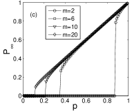
When the $n$ networks have the same average degree $k$, $k_{i}=k$ ($i=1,2,...,n$), using Eqs. (17) and (21) we obtain the percolation law for the order parameter, the size of the mutual giant components for all $p$ values and for all $k$ and $n$ gao2010 ,

$$\mu_{\infty,n}\equiv P_{\infty}=p[1-\exp(-kP_{\infty})]^{n}.$$ (27)

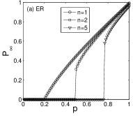
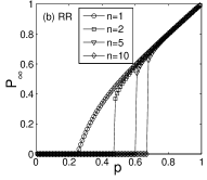
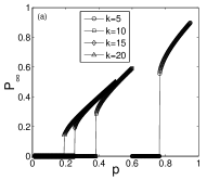
The solutions of equation (27) for several $n$-values are shown in Fig. 8(a). Results are in excellent agreement with simulations. The special case $n=1$ is the known ER second order percolation law for a single network ER1959 ; ER1960 ; Bollob1985 .

III.2 The case of NON with different average degrees

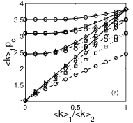
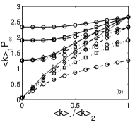
Next, we study the case where the average degrees of all $n$ networks is not the same. Without loss of generality we assume that $m$ networks have the same average degree $\langle k\rangle_{2}$, and other $n-m$ networks have the same average degree $\langle k\rangle_{1}$. We define $\alpha=\langle k\rangle_{1}/\langle k\rangle_{2}$ where $0<\alpha\leq 1$. Using Eqs. (16-19) we can show that $f_{c}$ satisfies

$$f_{c}=\exp[\frac{(f_{c}-1)(1-f_{c}^{1/\alpha})}{(n-m)f_{c}(1-f_{c}^{1/\alpha})+mf_{c}^{1/\alpha}(1-f_{c})/\alpha}].$$ (28)

Results for $p_{c}$ and the mutual giant component for different values of m, and alpha are shown in Fig. 11. The case of $\langle k\rangle_{1}\ll\langle k\rangle_{2}$ is interesting, since in this limit the $m$ networks with large $\langle k\rangle_{2}$ due to their good connectivity can not cause further damage to the $n-m$ networks with $\langle k\rangle_{1}$. Thus the NONs system can be regarded as only $n-m$ networks. Indeed, when $\alpha\rightarrow 0$, $f_{c}$ satisfies

$$f_{c}=e^{\frac{f_{c}-1}{(n-m)f_{c}}}.$$ (29)

And then equation of $p_{c}$ and $\mu_{\infty}$ are obtained as

$$p_{c}=[(n-m)\langle k\rangle_{1}f_{c}(1-f_{c})^{(n-m-1)}]^{-1},$$ (30)

and

$$\mu_{\infty}=\frac{1-f_{c}}{(n-m)\langle k\rangle_{1}f_{c}}.$$ (31)

Equations (29-31) are indeed the same as Eqs. (22, 24, and 25) where $n$ is replaced by $n-m$. This result is seen also in Fig. 11, where the limit of $\alpha=0$ yield the same results as for $\alpha=1$ for $n-m$ networks.

When $\langle k\rangle_{1}\ll\langle k\rangle_{2}$ for any $p$, we can get the equation of $P_{\infty}$ as a function of, $p$, $m$, $n$ and $\langle k\rangle_{1}$

$$P_{\infty}=p[1-\exp(-\langle k\rangle_{1}P_{\infty})]^{n-m}.$$ (32)

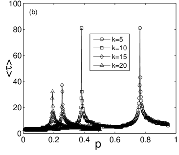
The average number of cascading stages, $\langle\tau\rangle$, as a function of $p$ for different value of average degree is shown in Fig. 11. The numerical simulation results show that $\tau$ increases sharply when $p$ is near $p_{c}$ parshani2010 .

Figure 8: Loopless NON is composed of (a) ER networks, (b) RR networks and (c) SF networks. Plotted is $P_{\infty}$ as a function of $p$ for $k=5$ (for ER and RR networks) and $\lambda=2.3$ for SF networks and several values of $n$. The results obtained using Eq. (27) for ER networks, Eq. (40) for RR networks and Eq. (51) for SF networks, agree well with simulations.

Figure 9: Loopless NON is composed of (a) ER networks, (b) RR networks and (c) SF networks. Plotted is $P_{\infty}$ as a function of $p$ for $n=5$ for several values of $k$ (ER and RR networks) and several values of $m$ (SF networks for $\lambda=2.3$). The results obtained using Eq. (27) for ER networks, Eq. (45) for RR networks and Eq. (56) for SF networks, agree well with simulations.

Figure 10: For star-like network of 5 ER networks, the average convergence stage $\langle\tau\rangle$ as a function of $p$ for different $k$. In the simulation, $N=10^{6}$, and the simulation results are obtained by over 30 realizations. This feature enables to find accurate estimate for $p_{c}$ in simulations parshani2010 .) agree well with simulations.

Figure 11: For loopless network of $n$ ER networks, $\langle k\rangle_{1}p_{c}$ and $\langle k\rangle_{1}\mu(\infty)$ as function of the ratio $\langle k\rangle_{1}/\langle k\rangle_{2}$ for $n=2$ (dashed), $n=3$ (dotted), $n=4$ (dashdot) and $n=5$ (solid) and for $m=1$ ($\circ$), $m=2$ ($\Box$), $m=3$ ($\diamond$) and $m=4$ ($\triangleright$), where $m$ denotes the number of individual networks whose average degree are the same $\langle k\rangle_{2}$ and average degree of the other $n-m$ networks are $\langle k\rangle_{1}$. The results are obtained using Eqs.(29)-(31).

IV ANALYTICAL RESULTS FOR THE CASE OF NON OF $n$ RR NETWORKS

Next, we study the case for a tree-like NON of $n$ RR networks. The degree of network $i$ is $k_{i}$. The generating functions of network $i$ are

$$G_{i,0}(x)=\sum k_{i}x^{k_{i}}=x^{k_{i}},$$ (33)

and

$$G_{i,1}(x)=x^{k_{i}-1}.$$ (34)

Using Eqs. (2) and (3), we obtain,

$$G_{i,0}(f,x)=(fx+1-x)^{k_{i}},$$ (35)

$$G_{i,1}(f,x)=(fx+1-x)^{k_{i}-1}.$$ (36)

For a single network $i$ we obtain $g_{i}(x)=1-G_{i,0}(f_{i},x)$, where $f_{i}$ satisfies the equation $f_{i}=G_{i,1}(f_{i},p)$. For loopless NON of $n$ networks, we can obtain

$$\mu^{\prime}_{i}=p\prod\limits_{j=1,j\neq i}^{n}[1-(f_{j}\mu^{\prime}_{j}+1-\mu^{\prime}_{j})^{k_{j}}],$$ (37)

where $f_{j}$ satisfies

$$f_{j}=[f_{j}\mu^{\prime}_{j}+1-\mu^{\prime}_{j}]^{k_{j}-1}.$$ (38)

Thus we can obtain

$$P_{\infty}\equiv\mu_{\infty}=p\prod\limits_{j=1}^{n}(1-f_{j}^{\frac{k_{j}}{k_{j}-1}}).$$ (39)

where $f_{i}$ satisfies

$$f_{i}=[(f_{i}-1)p\prod\limits_{j=1,j\neq i}^{n}(1-f_{j}^{\frac{k_{j}}{k_{j}-1}})+1]^{k_{i}-1}.$$ (40)

When all $n$ networks have the same degree $k$ i.e., $k_{i}=k$ ($i=1,2,...,n$), we introduce a new variables $r=f^{\frac{1}{k-1}}$ into Eq. (40), and the $n$ equations are reduced to a single one

$$r=(r^{k-1}-1)p(1-r^{k})^{n-1}+1,$$ (41)

which can be solved graphically for any $p$. The critical case corresponds to the tangential condition. Thus, we obtain that the value of $r$ satisfies a transcendental equation

$$1=(1-r)r^{k-2}[\frac{(n-1)kr}{1-r^{k}}+\frac{k-1}{1-r^{k-1}}].$$ (42)

Solving $r$ from Eq. (42), we can obtain the critical value of $p_{c}$ and the the value of $P_{\infty}$ at $p_{c}$ as

$$p_{c}=\frac{r-1}{(r^{k-1}-1)(1-r^{k})^{n-1}},$$ (43)

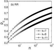
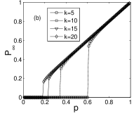
The numerical solutions are shown in Fig. 7(b).

$$P_{\infty}=p_{c}(1-r^{k})^{n}.$$ (44)

We can obtain $P_{\infty}$ as a function of $r$ by substituting $r$ into Eq. (41),

$$P_{\infty}=p\big{\{}1-\{p^{\frac{1}{n}}P_{\infty}^{\frac{n-1}{n}}[(1-(\frac{P_{\infty}}{p})^{\frac{1}{n}})^{\frac{k-1}{k}}-1]+1\}^{k}\big{\}}^{n}.$$ (45)

The results to compare the simulation and theory are shown in Fig. 6(a). The numerical simulation results is shown in Fig. 8(b) and 9(b).

For $n\gg 1$, Eq. (42) can be rewritten as

$$r=(\frac{1}{kn})^{\frac{1}{k-1}}.$$ (46)

From Eq. (43) and Eq. (46) for the case when $n\gg 1$, we obtain bashan2011

$$p_{c}=\frac{1-r}{e^{r/k}},$$ (47)

where $r$ satisfies Eq. (46).

Since $k/(1-k)<0$ for $k>1$, it follows, in contrast to the ER case, in the RR NON case $p_{c}$ can never be greater or equal to 1. This shows that an ER NON is extremely more vulnerable compared to RR NON, due to the critical role played in the ER by singly connected nodes.

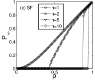
V ANALYTICAL RESULTS FOR THE CASE OF NON OF $n$ scale-free NETWORKS

Here we study the case of a tree-like NON composed of $n$ scale-free(SF) networks. The generating function of each network is

$$G_{i,0}(x)=\frac{\sum^{M}_{m}[(k+1)^{1-\lambda}-k^{1-\lambda}]x^{k}}{(M+1)^{1-\lambda}-m^{1-\lambda}},$$ (48)

$$G_{i,1}(x)=\frac{\sum^{M}_{m}[(k+1)^{1-\lambda}-k^{1-\lambda}]kx^{k-1}}{\sum^{M}_{m}[(k+1)^{1-\lambda}-k^{1-\lambda}]k},$$ (49)

and

$$G_{i,0}(f,x)=G_{i,0}(1+xf-x),$$ (50)

$$G_{i,1}(f,x)=G_{i,1}(1+xf-x).$$ (51)

$$g_{i}=1-G_{i,0}(1+xf-x).$$ (52)

$$f_{i}=G_{i,1}(1+xf-x).$$ (53)

Substituting Eq. (50) - (53) into Eqs. (8)-(10), we obtain

$$x=p\prod_{j\neq i}\Big{\{}1-\frac{\sum^{M_{j}}_{m_{j}}[(k+1)^{1-\lambda}-k^{1-\lambda}](1+f_{j}x_{j}-x_{j})^{k}}{(M+1)^{1-\lambda}-m^{1-\lambda}}\Big{\}},$$ (54)

$$f_{j}=\frac{\sum^{M_{j}}_{m_{j}}[(k+1)^{1-\lambda}-k^{1-\lambda}]k(1+f_{j}x_{j}-x_{j})^{k-1}}{\sum^{M}_{m}[(k+1)^{1-\lambda}-k^{1-\lambda}]k},$$ (55)

and

$$P_{\infty}=p\prod^{n}_{j=1}\Big{\{}1-\frac{\sum^{M_{j}}_{m_{j}}[(k+1)^{1-\lambda}-k^{1-\lambda}](1+f_{j}x_{j}-x_{j})^{k}}{(M+1)^{1-\lambda}-m^{1-\lambda}}\Big{\}}.$$ (56)

Figs. 8(c) and 9(c) show the solutions for $P_{\infty}$ for several values of $n$ and $m$ respectively.

VI The case when $n\rightarrow\infty$

The behavior of the networks for $n\to\infty$ depends only on $P(k)$, for small $k$.

If $P(1)+P(0)>0$, then no matter how large is $\langle k\rangle$ and what is the degree distribution for the rest of $k$, the networks completely collapse for large enough $n$ ($P_{\infty}=0$).

If $P(1)+P(0)=0$ the networks survive ($P_{\infty}>0$) for any $n$ and large enough $p<1$. Indeed, if $P(2)>0$ but $P(1)+P(0)=0$,

$$z_{c}\sim\frac{1}{n}(\frac{1}{2P(2)}-\frac{1}{\langle k\rangle}),$$ (57)

which corresponds to the maximum of the r.h.s of Eq. (12) and $p_{c}\to 1$, $P_{\infty}\to 1$ can be found from Eqs. (12) and (13). Thus, $p_{c}$ can not be greater than 1, meaning that for all $n$ values, the NON is stable.

Assuming $\sum_{0}^{\ell-1}P(k)=0$ and $P(\ell)>0$ then,

$$z_{c}\sim[1/(n\ell P(\ell))]^{1/(\ell-1)}.$$ (58)

and the way $p_{c}\to 1$ and $P_{\infty}\to 1$ can be found from Eqs. (12) and (13) to be.

$P_{\infty}=1-C_{1}/n^{1/(\ell-1)}$ and $p_{c}=1-C_{2}/n^{1/(\ell-1)}$, where $C_{1}>0$ and $C_{2}>0$ are constants, that can be easily found from Eqs. (12) and (13).

For $P(2)>0$, $C_{2}=2P(2)/\langle k\rangle^{2}$ and $C_{1}=(1-2P(2)/\langle k\rangle)^{2}/(2P(2))$ and for

$P(2)=0$, $C_{2}=(\ell-1)/(\ell P(\ell))^{1/(\ell-1)}$ and $C_{1}=1/(\ell P(\ell))]^{1/(\ell-1)}$. Thus, when $P(0)+P(1)=0$, the NON is stable for all $n$ ($p_{c}(n)<1$) and a condition for a minimal $k(n)$, such as in Eq. (26) does not exist.

VII Conclusion

In summary, we have developed a framework, Eqs. (9)-(10), for studying percolation of NON from which we derived an exact analytical law, Eqs. (27) [for ER networks] and (45) [for RR networks], for percolation in the case of a network of $n$ coupled networks. In particular for any $n\geq 2$, cascades of failures naturally appear and the phase transition becomes first order transition compared to a second order transition in the classical percolation of a single network. These findings show that the percolation theory of a single network is a limiting case of a more general case of percolation of interdependent networks. Due to cascading failures which increase with $n$, vulnerability significantly increases with $n$. We also find that for any tree-like network of networks the critical percolation threshold and the mutual giant component depend only on the number of networks and not on the topology (see Fig. 2). We discuss the case for $n$ coupled ER networks, RR networks and SF networks. We find that there exist the minimum $k$ to make the NON survives, but no parameter for the RR and SF networks.

VIII Appendix

VIII.1 The case when $n\rightarrow\infty$ for ER NON

Eq. (13) can be written as

$$n=\frac{f_{c}-1}{f_{c}\ln{f_{c}}}.$$ (59)

Then we can get,

$$\frac{dn}{df_{c}}=\frac{\ln{f_{c}}+1-f_{c}}{(f_{c}\ln{f_{c}})^{2}}.$$ (60)

When $n=1$,$f_{c}=1$, and $\frac{dn}{df_{c}}=0$; when $n>1$,$f_{c}<1$, and $\frac{dn}{df_{c}}<0$.

So $f_{c}$ is a decreasing function of $n$ when $n>1$. We introduce a new variable

$$\gamma=\frac{1-f_{c}}{nf_{c}},$$ (61)

so, $f_{c}=e^{-\gamma}$. When $n\rightarrow\infty$, $f_{c}\rightarrow 0$ and $\gamma\rightarrow\infty$. So studying the case $n\rightarrow\infty$ is the same as studying the case $\gamma\rightarrow\infty$.

Substitute Eq. (20) to Eq. (19), we obtain

$$n=\frac{1-e^{-\gamma}}{\gamma e^{-\gamma}}.$$ (62)

We study $n$ as a function of $\gamma$ when $\gamma\rightarrow\infty$,

$$\lim_{\gamma\rightarrow\infty}{n}=\frac{e^{\gamma}}{\gamma},$$ (63)

$$\ln{n}=\gamma-\ln{\gamma}.$$ (64)

Substituting Eq. (21) to Eq. (16) and consider the case when $\gamma\rightarrow\infty$, we obtain

$$k_{\min}=\frac{\gamma}{(1-e^{-\gamma})^{n}},$$ (65)

$$\lim_{\gamma\rightarrow\infty}{k_{\min}}=\frac{\gamma}{e^{\frac{1}{\gamma}}}.$$ (66)

Substituting Eq. (23a) to Eq. (22b) and consider the case when $\gamma\rightarrow\infty$, we obtain

$$k_{\min}=e^{-\frac{1}{\gamma}}\ln{n}+e^{-\frac{1}{\gamma}}\ln{k_{\min}}+\frac{1}{\gamma}e^{-\frac{1}{\gamma}},$$ (67)

$$\lim_{\gamma\rightarrow\infty}{k_{\min}}=\ln(n\ln{n})+\xi,$$ (68)

where $\xi=O(\ln(\ln{n}))$. We can also obtain that when $n\rightarrow\infty$, $p_{c}$ satisfies

$$p_{c}=\frac{1}{k}\ln(n\ln{n})+\xi,$$ (69)

where $\xi=O(\ln(\ln{n}))$. This result is corresponds to large $n$ values in Fig. 7(a).

References

- (1) Rinaldi S., Peerenboom J. & Kelly T. IEEE Contr. Syst. Mag. 21, 11-25 (2001).
- (2) Chang, S. E. The Bridge 39, 36-41 (2009).
- (3) Vespignani A. Nature 464, 984-985 (2010).
- (4) John S. Foster, Jr. et al. Critical National Infrastructures Report. Report: Electromagnetic Pulse (EMP) Attack (2008). (Online) Available: .
- (5) Rosato V. et al. Int. J. Crit. Infrastruct. 4, 63-79 (2008).
- (6) Buldyrev S. V. et al. Nature 464, 1025-1028 (2010).
- (7) Watts D. J. & Strogatz S. H. Nature 393, 440-442 (1998).
- (8) Albert R., Jeong H. & Barabási A. L. Nature 406, 378-382 (2000).
- (9) Cohen R. et al. Phys. Rev. Lett. 85, 4626–4628 (2000).
- (10) Callaway D. S. et al. Phys. Rev. Lett. 85, 5468-5471 (2000).
- (11) Albert R. & Barabási A. L. Rev. Mod. Phys. 74, 47-97 (2002).
- (12) Newman M. E. J. SIAM Review 45, 167-256 (2003).
- (13) Dorogovtsev S. N. & Mendes J. F. F. Evolution of Networks: From Biological Nets to the Internet and WWW (Physics) (Oxford Univ. Press, New York, 2003).
- (14) Song C. et al. Nature 433, 392-395 (2005).
- (15) Satorras R. P. & Vespignani A. Evolution and Structure of the Internet: A Statistical Physics Approach (Cambridge Univ. Press, England, 2006).
- (16) Caldarelli G. & Vespignani A. Large scale Structure and Dynamics of Complex Webs (World Scientific, 2007).
- (17) Barrát A., Barthélemy M. & Vespignani A. Dynamical Processes on Complex Networks (Cambridge Univ. Press, England, 2008).
- (18) Havlin S. & Cohen R. Complex Networks: Structure, Robustness and Function (Cambridge Univ. Press, England, 2010).
- (19) Newman M. E. J. Networks: An Introduction, (Oxford Univ. Press, New York, 2010).
- (20) Parshani R. et al. Phys. Rev. Lett. 105, 048701 (2010).
- (21) E. A. Leicht and R. M. D Souza, arXiv:cond-mat/0907.0894.
- (22) Peerenboom J., Fischer R. & Whitfield R. in Pro. CRIS/DRM/IIIT/NSF Workshop Mitigat. Vulnerab. Crit. Infrastruct. Catastr. Failures (2001).
- (23) J. Gao, S. V. Buldyrev, S. Havlin, H. E. Stanley. Robustness of a Network of Networks. arXive:1010.5829.
- (24) Erdős P. & Rényi A. I. Publ. Math. 6, 290-297 (1959).
- (25) Erdős P. & Rényi A. Publ. Math. Inst. Hung. Acad. Sci. 5, 17-61 (1960).
- (26) Bollobás B. Random Graphs (Academic, London, 1985).
- (27) Newman M. E. J. Strogatz S. H. & Watts D. J., Phys. Rev. E 64, 026118 (2001).
- (28) Newman M. E. J. Phys. Rev. E 66, 016128 (2002).
- (29) Shao J. et al. Europhys. Lett. 84, 48004 (2008).
- (30) Shao J. et al. Phys. Rev. E 80, 036105 (2009).
- (31) Lambert J. H. Acta Helveticae physico mathematico anatomico botanico medica, Band III, 128-168, (1758).
- (32) Corless R. M. et al. Adv. Computational Maths. 5, 329-359 (1996).
- (33) R. Parshani, S. V. Buldyrev, S. Havlin. Proc. Natl. Acad. Sci. USA 108, 1007 (2011).
- (34) Analogous results were found for a single network in the presence of dependency links (A. Bashan and S. Havlin., arXiv:1106.1631