Convergence of Rothe scheme for hemivariational inequalities of parabolic type

Abstract

This article presents the convergence analysis of a sequence of piecewise constant and piecewise linear functions obtained by the Rothe method to the solution of the first order evolution partial differential inclusion $u^{\prime}(t)+Au(t)+\iota^{*}\partial J(\iota u(t))\ni f(t)$, where the multivalued term is given by the Clarke subdifferential of a locally Lipschitz functional. The method provides the proof of existence of solutions alternative to the ones known in literature and together with any method for underlying elliptic problem, can serve as the effective tool to approximate the solution numerically. Presented approach puts into the unified framework known results for multivalued nonmonotone source term and boundary conditions, and generalizes them to the case where the multivalued term is defined on the arbitrary reflexive Banach space as long as appropriate conditions are satisfied. In addition the results on improved convergence as well as the numerical examples are presented.

1 Introduction

Partial differential inclusions with the multivalued term given in the form of Clarke subdifferential are known as hemivariational inequalities (HVIs). HVIs are the natural generalization of the inclusions with monotone multivalued term (which lead to variational inequalities) and were firstly considered by Panagiotopoulos in early 1980s. For the description of the origins of HVIs and underlying mathematical theory we refer the reader to the book [29].

This paper deals with the first order evolution inclusion of type $u^{\prime}(t)+A(u(t))+\iota^{*}\partial J(\iota u(t))\ni f(t)$. Such problems are known as parabolic HVIs or boundary parabolic HVIs depending whether an operator $\iota$ is the embedding operator from $H^{1}(\Omega)$ to $L^{2}(\Omega)$ or the trace operator from $H^{1}(\Omega)$ to $H^{\frac{1}{2}}(\partial\Omega)$. The first case corresponds to multivalued and nonmonotone source term in the equation and the second one to multivalued and nonmonotone boundary conditions of Neumann-Robin type. Such inclusions are used to model the diffusive transport through semipermeable membranes where the multivalued term represents the semipermeability relation [24] and the temperature control problems where the multivalued term represents the feedback control [16], [15].

The existence of solutions to problems governed by inclusions of considered type was investigated by many authors. There are several techniques used to obtain the existence results:

• Classical Faedo-Galerkin approach combined with the regularization of the multivalued term by means of a standard mollifier; solutions of underlying system of ordinary differential equations are proved to converge (in appropriate sense) to the function which is shown to be the solution of analyzed HVI. This technique was used in context of parabolic HVIs by Miettinen [22], Miettinen and Panagiotopoulos [24] and Goeleven et al. [14].

• The approach based on the notion of upper and lower solutions. The solution is shown to be the limit of solutions of problems governed by the equations obtained by the regularization of the multivalued term together with the truncation by the lower and upper solutions. The distinctive feature of this approach is that the growth conditions on the multivalued term are replaced by the assumption of the existence of lower and upper solutions. The technique was used for parabolic HVIs by Carl [4] and developed in [5], [6], [7], [9].

• The technique based on showing that the analyzed HVI satisfies the assumptions of the general framework for which the appropriate surjectivity result holds. This approach was used by Liu [19] and by Migórski [26] and developed for the boundary case in [27].

• The technique based on adding to the inclusion the regularizing term multiplied by $\epsilon>0$, showing that the solutions to obtained problems satisfy some bounds uniformly in $\epsilon$ and passing to the limit $\epsilon\to 0$. This technique was used for parabolic HVIs by Liu and Zhang [17] and Liu [18] and developed in [20], [21].

It should be remarked that above techniques are either nonconstructive (i.e. they are based on surjectivity result) or constructive but not effective (i.e. require a priori knowledge of lower and upper solutions, or require additional or smoothing terms in the problem).

In contrast to the existence theory, numerical methods to approximate effectively the solutions to parabolic HVIs were not considered by many authors. In the book of Haslinger, Miettinen and Panagiotopoulos [16] the convergence of solutions obtained by the finite element approximation of the space variable and finite difference approximation of the time variable is proved. However only the case of the linear operator $A$ and the multivalued source term (and not boundary conditions) is considered (see Remark 4.10 in [16]). In [15] the authors proved the convergence of the finite difference scheme (with respect to both time and space variable) for the case of multivalued source term (i.e. $U=H$ in the sequel).

Our approach uses the so-called Rothe method (known also as time approximation method) and allows to extend any numerical method that is used to solve the stationary, elliptic inclusions with the multivalued term given as the Clarke subdifferential, to time dependent, parabolic problems. The key idea is the replacement of time derivative with the backward difference scheme and solve the associated elliptic problem in every time step to find the solution in the consecutive points of the time mesh. It is proved that the results obtained by such approach approximate the solution of the original problem.

On the other hand, the Rothe metod provides the proof of existence of solutions. In contrast to other approaches this metod, as long as one can solve underlying elliptic problems, does not require any smoothing or other additional regularizing terms in the inclusion. Furthermore the presented approach allows to study the inclusions with multivalued term given on the domain and on the domain boundary within the unified framework in which the multifunction that appears in the problem is defined on an arbitrary reflexive Banach space, which satisfies the appropriate assumption ($H(U)$ in the sequel). This assumption is proved to generalize the case of inclusions with multivalued boundary conditions and the ones with multivalued source term (see Section 3 and examples of problem settings in Section 8).

The Rothe method for parabolic nonlinear PDEs with pseudomonotone operators is described in the monograph of Roubicek [33], where also the results for the monotone multivalued problems are presented. In the context of parabolic HVIs the variant of the Rothe method was used to show existence of solutions to problems with hysteresis in [23] and [25], but there only the case of linear operator $A$ and $f\in L^{2}(0,T;L^{2}(\Omega))$ (which excludes nonhomogeneous Neumann conditions) was considered and besides only the case of the multivalued and nonmonotone term source term was analyzed.

In Section 2 some basic definitions are recalled. Section 3 presents the generalization of the Lions-Aubin Compactness Lemma that justifies the usage of the assumption $H(U)$ in the sequel. Problem setup and the assumptions are presented in Section 4. The auxiliary elliptic problems solved in every time step, which are the key idea of the Rothe method, are formulated and analyzed in Section 5. Convergence of piecewise linear and piecewise constant functions constructed basing on the solutions of auxiliary problems as well as the fact that the limit solves the original problem is proved in Section 6. Some stronger convergence and uniqueness results are established in Section 7. Finally in Section 8 it is shown that the cases of multivalued boundary condition and source term are the special cases of presented general framework and a simple numerical example is delivered.

2 Preliminaries

In this section we recall several key definitions that will be used in the sequel.

For a locally Lipschitz functional $j:X\to\mathbb{R}$, where $X$ is a Banach space, generalized directional derivative (in the sense of Clarke) at $x\in X$ in the direction $z\in X$ is defined as

$$j^{0}(x;z)=\limsup_{y\to x,\lambda\to 0^{+}}\frac{j(y+\lambda z)-j(y)}{\lambda}.$$

Generalized gradient of $j$ (in the sense of Clarke) is the multifunction $\partial j:X\to 2^{X^{*}}$ defined by

$$\partial j(x)=\{\xi\in X^{*}:j^{0}(x;y)\geq\langle\xi,y\rangle\ \ \mbox{for all}\ \ y\in X\},$$

where $\langle\cdot,\cdot\rangle$ stands for the duality pairing between $X$ and $X^{*}$. For the properties and the calculus of the Clarke gradient see [10].

Recall that the multifunction $A:X\to 2^{X^{*}}$, where $X$ is a real and reflexive Banach space is pseudomonotone if

• $A$ has values which are nonempty, weakly compact and convex,

• $A$ is usc from every finite dimensional subsepace of $X$ into $X^{*}$ furnished with weak topology,

• if $v_{n}\to v$ weakly in $X$ and $v_{n}^{*}\in A(v_{n})$ is such that $\limsup_{n\to\infty}\langle v_{n}^{*},v_{n}-v\rangle\leq 0$ then for every $y\in X$ there exists $u(y)\in A(v)$ such that $\langle u(y),v-y\rangle\leq\liminf_{n\to\infty}\langle v_{n}^{*},v_{n}-y\rangle$.

Note that sometimes it is useful to check the pseudomonotonicity of an operator via the following sufficient condition (see Proposition 1.3.66 in [12] or Proposition 3.1 in [8]).

Proposition 1.

Let X be a real reflexive Banach space, and assume that $A:X\to 2^{X^{*}}$ satisfies the following conditions

• for each $v\in X$ we have that $A(v)$ is a nonempty, closed and convex subset of $X^{*}$.

• $A$ is bounded.

• If $v_{n}\to v$ weakly in $X$ and $v_{n}^{*}\to v^{*}$ weakly in $X^{*}$ with $v_{n}^{*}\in A(v_{n})$ and if $\limsup_{n\to\infty}\langle v_{n}^{*},v_{n}-v\rangle\leq 0$, then $v^{*}\in A(v)$ and $\langle v_{n}^{*},v_{n}\rangle\to\langle v^{*},v\rangle$.

Then the operator $A$ is pseudomonotone.

We also recall (see for instance Proposition 1.3.68 [12]) that the sum of two pseudomonotone multifunctions is pseudomonotone.

3 Generalization of Lions-Aubin Lemma

For a Banach space $X$, $1\leq p\leq\infty$ and a finite time interval $I=(0,T)$ we consider the standard spaces $L^{p}(I;X)$. Furthermore we denote by $BV(I;X)$ the space of functions of bounded total variation on $I$. Let $\pi$ denote any finite partition of $I$ by a family of disjoint subintervals $\{\sigma_{i}=(a_{i},b_{i})\}$ such that $\bar{I}=\bigcup_{i=1}^{n}\bar{\sigma}_{i}$. Let ${\mathcal{F}}$ denote the family of all such partitions. Then we define the total variation as

$$\|x\|_{BV(I;X)}=\sup_{\pi\in{\mathcal{F}}}\left\{\sum_{\sigma_{i}\in\pi}\|x(b_{i})-x(a_{i})\|_{X}\right\}.$$

As a generalization of above definition for $1\leq q<\infty$ we can define a seminorm

$$\|x\|_{BV^{q}(I;X)}^{q}=\sup_{\pi\in{\mathcal{F}}}\left\{\sum_{\sigma_{i}\in\pi}\|x(b_{i})-x(a_{i})\|^{q}_{X}\right\}.$$

For Banach spaces $X,Z$ such that $X\subset Z$ we introduce a vector space

$$M^{p,q}(I;X,Z)=L^{p}(I;X)\cap BV^{q}(I;Z).$$

Then $M^{p,q}(I;X,Z)$ is also a Banach space for $1\leq p,q<\infty$ with the norm given by $\|\cdot\|_{L^{p}(I;X)}+\|\cdot\|_{BV^{q}(I;Z)}$.

Let us recall Theorem 1 of [34] (see also Theorem 1 of [32] and Proposition 2.1 of [31]).

Theorem 1.

Let $1\leq p<\infty$ and $X$ be a real Banach space. A subset ${\mathcal{G}}\subset L^{p}(0,T;X)$ is relatively compact in a Banach space $L^{p}(0,T;X)$ provided the following two conditions hold

• for every $0<t_{1}<t_{2}<T$ the set

  $$G(t_{1},t_{2}):=\left\{\int_{t_{1}}^{t_{2}}u(t)\,dt:u\in{\mathcal{G}}\right\}$$

  is relatively compact in $X$,

• ${\mathcal{G}}$ is strongly integrally equicontinuous i.e.

  $$\lim_{h\to 0}\sup_{u\in{\mathcal{G}}}\int_{0}^{T-h}\|u(t+h)-u(t)\|_{X}^{p}\ dt=0.$$ (1)

The following proposition is a consequence of Theorem 1.

Proposition 2.

Let $1\leq p,q<\infty$. Let $X_{1}\subset X_{2}\subset X_{3}$ be real Banach spaces such that $X_{1}$ is reflexive, the embedding $X_{1}\subset X_{2}$ is compact and the embedding $X_{2}\subset X_{3}$ is continuous. If a subset ${\mathcal{G}}\subset M^{p,q}(I;X_{1},X_{3})$ is bounded, then it is relatively compact in $L^{p}(I;X_{2})$.

Proof.

We apply Theorem 1 with $X=X_{2}$. Let us fix $0<t_{1}<t_{2}<T$ and let $v\in G(t_{1},t_{2})$. For $u\in{\mathcal{G}}$ we have

$$\|v\|_{X_{1}}=\left\|\int_{t_{1}}^{t_{2}}u(t)\,dt\right\|_{X_{1}}\leq\int_{0}^{T}\|u(t)\|_{X_{1}}\,dt\leq T^{1-\frac{1}{p}}\|u\|_{L^{p}(I;X_{1})}.$$ (2)

Thus $G(t_{1},t_{2})$ is bounded in $X_{1}$ and therefore relatively compact in $X_{2}$.

It suffices to show the strong integral equicontinuity of ${\mathcal{G}}$. Let $\sup_{u\in{\mathcal{G}}}\|u\|_{L^{p}(I;X_{1})}^{p}=M$. We will use the Ehrling Lemma (see for instance [33], Lemma 7.6). Let us fix $\varepsilon>0$. There exists $C>0$ such that for $v\in X_{1}$ we have $\|v\|_{X_{2}}^{p}\leq\frac{\varepsilon}{2^{p}M}\|v\|_{X_{1}}^{p}+C\|v\|_{X_{3}}^{p}$. In particular, fixing $h\in(0,T)$, for $u\in{\mathcal{G}}$ and almost every $t\in(0,T-h)$ we have $\|u(t+h)-u(t)\|_{X_{2}}^{p}\leq\frac{\varepsilon}{2^{p}M}\|u(t+h)-u(t)\|_{X_{1}}^{p}+C\|u(t+h)-u(t)\|_{X_{3}}^{p}$. Integrating this inequality we get

$$\int_{0}^{T-h}\|u(t+h)-u(t)\|_{X_{2}}^{p}\ dt\leq$$

$$\leq\frac{\varepsilon}{2^{p}M}\int_{0}^{T-h}\|u(t+h)-u(t)\|_{X_{1}}^{p}\ dt+C\int_{0}^{T-h}\|u(t+h)-u(t)\|_{X_{3}}^{p}\ dt\leq$$

$$\leq\frac{\varepsilon}{2M}\int_{0}^{T-h}\|u(t+h)\|_{X_{1}}^{p}+\|u(t)\|_{X_{1}}^{p}\ dt+C\int_{0}^{T-h}\|u(t+h)-u(t)\|_{X_{3}}^{p}\ dt\leq$$

$$\leq\varepsilon+C\int_{0}^{T-h}\|u(t+h)-u(t)\|_{X_{3}}^{p}\ dt.$$ (3)

Now let $\sup_{u\in{\mathcal{G}}}\|u\|_{BV^{q}(I;X_{3})}^{q}=S$. If $p\leq q$, then by the Hölder inequality, we have

$$\int_{0}^{T-h}\|u(t+h)-u(t)\|_{X_{3}}^{p}\ dt\leq T^{1-\frac{p}{q}}\left(\int_{0}^{T-h}\|u(t+h)-u(t)\|_{X_{3}}^{q}\ dt\right)^{\frac{p}{q}}.$$ (4)

If in turn $q<p$, then

$$\int_{0}^{T-h}\|u(t+h)-u(t)\|_{X_{3}}^{p}\ dt\leq S^{\frac{p}{q}-1}\int_{0}^{T-h}\|u(t+h)-u(t)\|_{X_{3}}^{q}\ dt.$$ (5)

We estimate the last term in (4) and (5) from above (taking, if necessary, $u(t)=u(T)$, if $t>T$)

$$\int_{0}^{T-h}\|u(t+h)-u(t)\|_{X_{3}}^{q}\ dt\leq\sum_{i=0}^{\lceil T/h-2\rceil}\int_{ih}^{ih+h}\|u(t+h)-u(t)\|_{X_{3}}^{q}\ dt=$$

$$=\sum_{i=0}^{\lceil T/h-2\rceil}\int_{0}^{h}\|u(t+ih+h)-u(t+ih)\|_{X_{3}}^{q}\ dt=$$

$$=\int_{0}^{h}\sum_{i=0}^{\lceil T/h-2\rceil}\|u(t+ih+h)-u(t+ih)\|_{X_{3}}^{q}\ dt\leq Sh.$$ (6)

Thus the last term in (3) tends to $0$ uniformly in $u$ as $h\to 0$ and, since $\varepsilon$ was arbitrary, we get the thesis. ∎

Remark 1. Note, that Theorem 3.2 in [1] is a consequence of above theorem. Compare also the Corollary 7.9 in [33] where the case $p=1$ is excluded and $X_{3}$ is assumed to have a predual space.

4 Problem formulation and assumptions

Let $V\subset H\subset V^{*}$ be an evolution triple, where $V$ is a reflexive and separable Banach space and $H$ is a separable Hilbert space with the embeddings being continuous, dense and compact. Embedding between $V$ and $H$ will be denoted by $i$. Furthermore let $U$ be a reflexive Banach space on which the multivalued term will be defined. We use the notation ${\mathcal{V}}=L^{2}(0,T;V)$, ${\mathcal{H}}=L^{2}(0,T;H)$, ${\mathcal{U}}=L^{2}(0,T;U)$ and ${\mathcal{W}}=\{u\in{\mathcal{V}},u^{\prime}\in{\mathcal{V}}^{*}\}$, where the derivative is understood in the sense of distibutions. Duality parings and norms for all the spaces will be denoted by the appropriate subscripts, for the space $V$ no subscript will be used. Scalar product in $H$ will be denoted by $(\cdot,\cdot)$ and norm in $\mathbb{R}^{n}$ by $|\cdot|$. We consider the operator $A:V\to V^{*}$ and the functional $J:U\to\mathbb{R}$ such that the following assumptions hold

• • $A$ is pseudomonotone,

  • $A$ satisfies the growth condition $\|A(v)\|_{V^{*}}\leq a+b\|v\|$ for every $v\in V$ with $a\geq 0,b>0$,

  • $A$ is coercive $\langle A(v),v\rangle\geq\alpha\|v\|^{2}-\beta\|v\|^{2}_{H}$ for every $v\in V$ with $\alpha>0$ and $\beta\geq 0$,

• • $J$ is locally Lipschitz,

  • $\partial J$ satisfies the growth condition $\|\xi\|_{U^{*}}\leq c(1+\|u\|_{U})$ for every $u\in U$ and $\xi\in\partial J(u)$ with $c>0$.

Moreover we assume that

• $f\in{\mathcal{V}}^{*}$ and $u_{0}\in H$.

We also impose the assumption concerning the space $U$

• There exists the linear, continuous and compact mapping $\iota:V\to U$ such that the associated Nemytskii mapping $\bar{\iota}:M^{2,2}(0,T;V,V^{*})\to{\mathcal{U}}$ defined by $(\bar{\iota}v)(t)=\iota(v(t))$ is also compact.

Finally we impose the last assumption

• One of the following holds

  • There exists a linear and continuous mapping $p:H\to U$ such that for $v\in V$ we have $p(i(v))=\iota(v)$.

  • The constants $\alpha$ and $c$ satisfy the inequality $\alpha>c\|\iota\|_{{\mathcal{L}}(V;U)}^{2}$.

  • For every $u\in U$ we have $J^{0}(u;-u)\leq d(1+\|u\|_{U}^{\sigma})$ with $d\geq 0$ and $1\leq\sigma<2$.

The problem under consideration is as follows

$$\mbox{find}\ u\in{\mathcal{W}}\ \mbox{such that}\ u(0)=u_{0}\ \mbox{and for a.e.}\ t\in(0,T)\ \mbox{we have}$$

$$u^{\prime}(t)+Au(t)+\iota^{*}\partial J(\iota u(t))\ni f(t).$$ (7)

The last inclusion is understood in the following sense

$$\mbox{there exists}\ \ \eta\in{\mathcal{V}}^{*}\ \mbox{such that}\ u^{\prime}(t)+Au(t)+\eta(t)=f(t)\ \mbox{for a.e.}\ t\in(0,T)$$

$$\mbox{and}\ \ \langle\eta(t),v\rangle\in\langle\partial J(\iota u(t)),\iota v\rangle_{U^{*}\times U}\ \mbox{for a.e.}\ t\in(0,T)\ \mbox{and}\ v\in V.$$ (8)

Remark 2. The formulation (7) puts into a unified framework hemivariational inequalities originating from the initial and boundary value problem with multivalued term defined on the problem domain (in this case we have multivalued source term, and $U=H$, see [22, 24, 26]) and on the part $\Gamma_{C}$ of domain boundary $\partial\Omega$ (this is the case if we have the multivalued, nonlinear and nonmonotone boundary condition of Neumann-Robin type, $U=L^{2}(\Gamma_{C})$ or $U=L^{2}(\Gamma_{C};\mathbb{R}^{n})$, see [27]). A detailed discussion as well as examples of problems which satisfy the assumptions will be given in Section 8.

Remark 3. For the sake of simplicity of further argument the assumptions given above are not the most general ones under which the results hold. Possible generalizations include:

• The dependance of $A$ and $J$ on time variable. Time dependent operator $A$ for parabolic HVI is considered in [24] and the case of both $A$ and $J$ depending on time is considered in [27] (see Remark 8.21 in [33] on the Rothe method for the problem with the operator depending on time).

• Instead of pseudomonotonicity one could assume that $A$ is a sum of two operators, one of which is pseudomonotone and the second one is weakly continuous. Such weak continuity allows to take into account the nonlinear terms of lower order which are not of monotone type (see [13]).

• More general coercivity conditions on $A$ can be assumed. For instance $\langle Av,v\rangle\geq c\|v\|^{2}-a\|v\|_{V}-\gamma(t)$ with $c>0$, $a\geq 0$ and $\gamma\in L^{1}(0,T)$ cf. [26].

• The case when the space ${\mathcal{V}}$ is defined as $L^{p}(0,T;V)$ with $2<p<\infty$ can be considered. Then we can assume more general growth conditions on $A$ and $J$. For instance in [26] it is assumed that $\|A(t,v)\|_{V^{*}}\leq\beta(t)+c_{1}\|v\|^{p-1}$ and that for $\eta\in\partial j(x,\xi)$ we have $|\eta|\leq c(1+|\xi|^{p-1})$. Note that $J$ is defined typically as the integral functional $J(u)=\int_{\omega}j(x,u(x))\,dx$ and assumptions on the integrand $j$ are given.

Remark 4. In this paper the abstract setting is considered. For a divergence differential operator of Leray - Lions type on a Sobolev space pseudomonotnicity is implied by the appropriate Leray - Lions type conditions (see, for instance, [3] where conditions that guarantee pseudomonotonicity on $W^{m,p}(\Omega)$, $1<p<\infty$, $m\geq 1$ are considered).

We conclude this section with the Lemma on pseudomonotonicity of Nemytskii operator with respect to the space $M^{2,2}(0,T;V,V^{*})$. Note that the proof of this lemma is analogous to the proof of Theorem 2 (b) in [3] (see also Proposition 1 from [30] and Lemma 8.8 in [33] for similar results). Lemma 8.8 of [33] is most similar to Lemma 1, but note that here no a priori bound in $L^{\infty}(0,T;H)$ is needed and the assumption on the bound of 2-variation which is used here is weaker then the bound on 1-variation as in [33].

Lemma 1.

Let $A:V\to V^{*}$ satisfy $H(A)$ and let ${\mathcal{A}}:{\mathcal{V}}\to{\mathcal{V}}^{*}$ be a Nemytskii operator for $A$ defined by $({\mathcal{A}}u)(t)=A(u(t))$. Then if, for a uniformly bounded sequence $\{u_{n}\}\subset M^{2,2}(0,T;V,V^{*})$ such that $u_{n}\to u$ weakly in ${\mathcal{V}}$ we have $\limsup_{n\to\infty}\langle{\mathcal{A}}u_{n},u_{n}-u\rangle_{{\mathcal{V}}^{*}\times{\mathcal{V}}}\leq 0$, then ${\mathcal{A}}u_{n}\to{\mathcal{A}}u$ weakly in ${\mathcal{V}}^{*}$.

Proof.

It is enough to show that the thesis holds for a subsequence. By the generalized Lions Aubin Compactness Lemma (see Proposition 2) for a subsequence (still denoted by $n$) we have $u_{n}\to u$ strongly in ${\mathcal{H}}$. Moreover, for yet another subsequence $u_{n}(t)\to u(t)$ strongly in $H$ for a.e. $t\in(0,T)$. We denote the set of measure zero on which the convergence does not hold by $N$. Now let us define $\xi_{n}(t)=\langle Au_{n}(t),u_{n}(t)-u(t)\rangle$. We have

$$\xi_{n}(t)\geq\alpha\|u_{n}(t)\|^{2}-\beta\|u_{n}(t)\|_{H}^{2}-\|u(t)\|(a+b\|u_{n}(t)\|)\geq$$ (9)

$$\geq\frac{\alpha}{2}\|u_{n}(t)\|^{2}-\beta\|u_{n}(t)\|_{H}^{2}-a\|u(t)\|-\frac{b^{2}}{2\alpha}\|u(t)\|^{2}.$$

Now let $C=\{t\in[0,T]:\liminf_{n\to\infty}\xi_{n}(t)<0\}$. This is the Lebesgue measurable subset of $[0,T]$. Suppose that $m(C)>0$, $m$ being one dimensional Lebesgue measure. For every $t\in C\setminus N$ the sequence $u_{n}(t)$ has a subsequence (still denoted by $n$) which is bounded in $V$ by (9) such that $\lim_{n\to\infty}\langle Au_{n}(t),u_{n}(t)-u(t)\rangle<0$. Again for a subsequence we have $u_{n}(t)\to u(t)$ weakly in $V$, where the limit equals $u(t)$ since we can consider only $t\notin N$. By the pseudomonotonicity of $A$ we get $0\leq\liminf_{n\to\infty}\langle Au_{n}(t),u_{n}(t)-u(t)\rangle$, which is a contradiction. So $m(C)=0$, which means that $\liminf_{n\to\infty}\xi_{n}(t)\geq 0$ a.e. on $(0,T)$. From the Fatou Lemma we have

$$\beta\|u\|_{H}^{2}\leq\int_{0}^{T}\liminf_{n\to\infty}\xi_{n}(t)\,dt+\beta\|u\|_{H}^{2}\leq\int_{0}^{T}\liminf_{n\to\infty}(\xi_{n}(t)+\beta\|u_{n}(t)\|_{H}^{2})\,dt\leq$$

$$\leq\liminf_{n\to\infty}\int_{0}^{T}\xi_{n}(t)+\beta\|u_{n}(t)\|_{H}^{2}\,dt\leq$$

$$\leq\liminf_{n\to\infty}\int_{0}^{T}\xi_{n}(t)\,dt+\beta\|u\|_{H}^{2}\leq\limsup_{n\to\infty}\int_{0}^{T}\xi_{n}(t)\,dt+\beta\|u\|_{H}^{2}\leq\beta\|u\|_{H}^{2}.$$

So $\int_{0}^{T}\xi_{n}(t)\,dt\to 0$ as $n\to\infty$. Now note that $|\xi_{n}(t)|=\xi_{n}(t)+2\xi_{n}^{-}(t)$ and $\xi_{n}^{-}(t)\to 0$ for a.e. $t\in(0,T)$. Since, by (9), for a.e. $t\in(0,T)$ we have $\xi_{n}(t)+\beta\|u_{n}(t)\|_{H}^{2}\geq f(t)$ with $f\in L^{1}(0,T)$, then $\xi_{n}^{-}(t)-\beta\|u_{n}(t)\|_{H}^{2}\leq f^{-}(t)$. Invoking Fatou Lemma again we have $\limsup\int_{0}^{T}\xi^{-}(t)\,dt\leq 0$ and furthermore $\int_{0}^{T}\xi_{n}^{-}(t)\,dt\to 0$ as $n\to\infty$. We deduce that $\xi_{n}\to 0$ in $L^{1}(0,T)$ and, for a subsequence (still denoted by the same subscript), $\xi_{n}(t)\to 0$ for a.e. $t\in(0,T)$. Since, for this subsequence, $u_{n}(t)\to u(t)$ weakly in $V$, then by pseudomonotonicity of $A$ it follows that $Au_{n}(t)\to Au(t)$ weakly in $V^{*}$ and $\langle Au_{n}(t),u_{n}(t)\rangle\to\langle Au(t),u(t)\rangle$. For any $v\in{\mathcal{V}}$ we have

$$\langle{\mathcal{A}}u,u-v\rangle_{{\mathcal{V}}^{*}\times{\mathcal{V}}}=\int_{0}^{T}\langle Au(t),u(t)-v(t)\rangle\,dt=\int_{0}^{T}\lim_{n\to\infty}\langle Au_{n}(t),u_{n}(t)-v(t)\rangle\,dt=$$

$$=-\beta\|u\|_{H}^{2}+\int_{0}^{T}\lim_{n\to\infty}(\langle Au_{n}(t),u_{n}(t)-v(t)\rangle+\beta\|u_{n}(t)\|_{H}^{2})\,dt.$$

We can apply Fatou Lemma one last time to get

$$\langle{\mathcal{A}}u,u-v\rangle_{{\mathcal{V}}^{*}\times{\mathcal{V}}}\leq\liminf_{n\to\infty}\int_{0}^{T}\langle Au_{n}(t),u_{n}(t)-v(t)\rangle\,dt=$$

$$=\liminf_{n\to\infty}(\langle{\mathcal{A}}u_{n},u_{n}-u\rangle_{{\mathcal{V}}^{*}\times{\mathcal{V}}}+\langle{\mathcal{A}}u_{n},u-v\rangle_{{\mathcal{V}}^{*}\times{\mathcal{V}}})\leq$$

$$\leq\liminf_{n\to\infty}\langle{\mathcal{A}}u_{n},u-v\rangle_{{\mathcal{V}}^{*}\times{\mathcal{V}}}.$$ (10)

Since $v$ is arbitrary we obtain the thesis. ∎

5 The Rothe problem

In this section we will work with a sequence of time-steps $\tau_{n}\to 0$ such that each time step $\tau_{n}>0$ and the value $T/\tau_{n}$ is an integer, which we denote by $N_{n}$. The subscipt $n$ will be omitted in the sequel in order to simplify the notation, so we will write $N,\tau$ instead of $N_{n},\tau_{n}$.

We define the piecewise constant approximation of the function $f\in{\mathcal{V}}^{*}$. For this purpose we take the sequence of positive numbers $\epsilon(\tau)\to 0$ and the sequence of mollifiers $\rho_{\epsilon}:\mathbb{R}\to\mathbb{R}$ which belong to $C^{\infty}(\mathbb{R})$ and are nonnegative, supported on $[-\epsilon,\epsilon]$ and $\int_{\mathbb{R}}\rho_{\epsilon}(x)\,dx=1$. The function $f$ is regularized according to the formula

$$f_{\epsilon}(t)=\int_{0}^{T}\rho_{\epsilon}\left(t+\epsilon\frac{T-2t}{T}-s\right)f(s)\,ds.$$

Note that $f_{\epsilon}\in C^{1}(0,T;V^{*})$ (see [33], Lemma 7.2). The piecewise constant approximation for $f$ is given by

$$\bar{f}_{\tau}(t):=f^{k}_{\tau}=f_{\epsilon(\tau)}(k\tau)\ \mbox{for}\ t\in((k-1)\tau,k\tau],\ k\in\{1,\ldots,N\}.$$

Following [33], Lemma 8.7, we have $\bar{f}_{\tau}\to f$ in ${\mathcal{V}}^{*}$ when $\tau\to 0$. Note (see Remark 8.15 in [33]) that the smoothing of $f$ is not the only possible approach here. It is also possible to take the Clément zero-order quasi interpolant $f_{\tau}^{k}=\frac{1}{\tau}\int_{(k-1)\tau}^{k\tau}f(\theta)\,d\theta$.

We approximate the initial condition by elements of $V$. Let $\{u_{0\tau}\}\subset V$ be a sequence such that $u_{0\tau}\to u_{0}$ strongly in $H$ and $\|u_{0\tau}\|\leq C/\sqrt{\tau}$ for some constant $C>0$.

We define the following Rothe problem

$$\mbox{find the sequence}\ \{u_{\tau}^{k}\}_{k=0}^{N}\subset V\ \mbox{such that}\ u_{\tau}^{0}=u_{0\tau}\ \mbox{and}$$

$$\left(\frac{u^{k}_{\tau}-u^{k-1}_{\tau}}{\tau},v\right)_{H}+\langle Au_{\tau}^{k},v\rangle+\langle\partial J(\iota u^{k}_{\tau}),\iota v\rangle_{U^{*}\times U}\ni\langle f^{k}_{\tau},v\rangle$$ (11)

$$\mbox{for all}\ v\in V\ \mbox{and}\ k=1,\ldots,N.$$

The above formula is known as the implicit or backward Euler scheme. Existence of solutions to the Rothe problem follows from the following

Lemma 2.

Under assumptions $H(A),H(J),H_{0},H(U)$ and $H_{aux}$ there exists $\tau_{0}>0$ such that the problem (11) has a solution for $\tau\in(0,\tau_{0})$.

Proof.

We show that, given $u^{k-1}_{\tau}\in V$, we can find $u^{k}_{\tau}\in V$ such that (11) holds. We need to show that the range of multifunction $V\ni v\to Lv=\frac{i^{*}iv}{\tau}+Av+\iota^{*}\partial J(\iota v)\in 2^{V^{*}}$ constitutes the whole space $V^{*}$. We will use the surjectivity theorem for pseudomonotone operators (see for instance Theorem 1.3.70 in [12]). We need to show that $L$ is coercive (in the sense that $\lim_{\|v\|\to\infty}\frac{\inf_{v^{*}\in Lv}\langle v^{*},v\rangle}{\|v\|}=\infty$) and pseudomonotone.

Claim 1. $L$ is pseudomonotone. We verify this condition for all components of $L$ separately. For this purpose we use Proposition 1. The operator $\frac{i^{*}i}{\tau}$ satisfies the conditions $(i)-(iii)$ trivially. As for $\iota^{*}\partial J(\iota u)$ the condition $(i)$ follows from the fact that the Clarke subdifferential has nonempty, convex and (for reflexive space) weakly compact values. The condition $(ii)$ follows from the growth assumption on $\partial J$. In order to verify $(iii)$ let us take $v_{n}\to v$ weakly in $V$ and $\xi_{n}\to\xi$ weakly in $V^{*}$ with $\xi_{n}\in\iota^{*}\partial J(\iota v_{n})$. Obviously $\iota v_{n}\to\iota v$ strongly in $U$. Define $\eta_{n}\in\partial J(\iota v_{n})$ such that $\xi_{n}=\iota^{*}\eta_{n}$. By the growth condition $H(J)(ii)$ it follows that, for a subsequence still denoted by the same subscript, $\eta_{n}\to\eta$ weakly in $U^{*}$. By the closedness of the graph of $\partial J$ in $U\times U^{*}_{w}$ topology (see [10], Proposition 2.1.5), we get $\eta\in\partial J(\iota v)$. Obviously $\xi=\iota^{*}\eta$ and $\xi\in\iota^{*}\partial J(\iota v)$. Moreover $\langle v_{n},\xi_{n}\rangle=\langle\iota v_{n},\eta_{n}\rangle_{U^{*}\times U}\to\langle\iota v,\eta\rangle_{U^{*}\times U}=\langle v,\xi\rangle$, where by uniqueness convergence holds for the whole sequence.

Claim 2. $L$ is coercive. Assume that $v^{*}\in Lv$. We estimate $\langle v^{*},v\rangle$ from below. For some $\eta\in\partial J(\iota v)$ we have

$$\langle v^{*},v\rangle\geq\frac{1}{\tau}\|v\|_{H}^{2}+\alpha\|v\|^{2}-\beta\|v\|_{H}^{2}+\langle\eta,\iota v\rangle_{U^{*}\times U}.$$ (12)

We proceed for cases $A),B),C)$ separately. For $A)$ and $B)$, by the growth condition

$$\langle v^{*},v\rangle\geq\left(\frac{1}{\tau}-\beta\right)\|v\|_{H}^{2}+\alpha\|v\|^{2}-c(1+\|\iota v\|_{U})\|\iota v\|_{U}.$$

In the case $A)$ we have $\|\iota v\|_{U}^{2}\leq\|p\|_{{\mathcal{L}}(H,U)}^{2}\|v\|_{H}^{2}$, so

$$\langle v^{*},v\rangle\geq\left(\frac{1}{\tau}-\beta-c\|p\|_{{\mathcal{L}}(H,U)}^{2}\right)\|v\|_{H}^{2}+\alpha\|v\|^{2}-c\|\iota\|_{{\mathcal{L}}(V;U)}\|v\|.$$

We require $\tau_{0}=\frac{1}{\beta+c\|p\|_{{\mathcal{L}}(H,U)}}$. In the case $B)$ we get

$$\langle v^{*},v\rangle\geq\left(\frac{1}{\tau}-\beta\right)\|v\|_{H}^{2}+(\alpha-c\|\iota\|^{2}_{{\mathcal{L}}(V;U)})\|v\|^{2}-c\|\iota\|_{{\mathcal{L}}(V;U)}\|v\|.$$

To have coercivity we need to set $\tau_{0}=\frac{1}{\beta}$. Finally if $C)$ holds, then we get

$$\langle\eta,\iota v\rangle_{U^{*}\times U}\geq-J^{0}(\iota v;-\iota v)\geq$$

$$\geq-d(1+\|\iota v\|_{U}^{\sigma})\geq-d-\|\iota\|_{{\mathcal{L}}(V;U)}^{\sigma}\|v\|^{\sigma}\geq-d-\frac{\alpha}{2}\|v\|^{2}-C,$$

where $C>0$ depends on $\alpha,\sigma$ and $\|\iota\|_{{\mathcal{L}}(V;U)}$. Combining the last estimate with (12) we get

$$\langle v^{*},v\rangle\geq\left(\frac{1}{\tau}-\beta\right)\|v\|_{H}^{2}+\frac{\alpha}{2}\|v\|^{2}-d-C.$$

Again setting $\tau_{0}=\frac{1}{\beta}$ we get the desired property. ∎

Next lemma establishes the estimates which are satisfied by the solutions of Rothe problem.

Lemma 3.

Under assumptions $H(A),H(J),H_{0},H(U)$ and $H_{aux}$ there exists $\tau_{0}>0$ such that for all $\tau\in(0,\tau_{0})$ the solutions of Rothe problem (11) satisfy

$$\max_{k=1,\ldots,N}\|u_{\tau}^{k}\|_{H}\leq\mbox{const},$$ (13)

$$\sum_{k=1}^{N}\|u_{\tau}^{k}-u_{\tau}^{k-1}\|_{H}^{2}\leq\mbox{const},$$ (14)

$$\tau\sum_{k=1}^{N}\|u_{\tau}^{k}\|^{2}\leq\mbox{const},$$ (15)

with the constants independent on $\tau$.

Proof.

We take $v=u^{k}_{\tau}$ in (11), which gives for $\varepsilon>0$ and $k=1,\ldots,N$

$$\frac{1}{\tau}\|u^{k}_{\tau}\|^{2}_{H}+\alpha\|u^{k}_{\tau}\|^{2}+\langle\xi_{\tau}^{k},\iota u^{k}_{\tau}\rangle_{U^{*}\times U}\leq$$

$$\leq\beta\|u^{k}_{\tau}\|_{H}^{2}+\frac{1}{2\varepsilon}\|f^{k}_{\tau}\|^{2}_{V^{*}}+\frac{\varepsilon}{2}\|u^{k}_{\tau}\|^{2}+\frac{1}{\tau}(u^{k-1}_{\tau},u^{k}_{\tau})$$

with $\xi_{\tau}^{k}\in\partial J(\iota u^{k}_{\tau})$. We use the relation $\|a\|^{2}-(a,b)=\|a\|^{2}/2-\|b\|^{2}/2+\|a-b\|^{2}/2$ to obtain

$$\left(\frac{1}{2\tau}-\beta\right)\|u^{k}_{\tau}\|^{2}_{H}+\frac{1}{2\tau}\|u^{k}_{\tau}-u^{k-1}_{\tau}\|_{H}^{2}+\left(\alpha-\frac{\varepsilon}{2}\right)\|u^{k}_{\tau}\|^{2}+$$ (16)

$$+\langle\xi_{\tau}^{k},\iota u^{k}_{\tau}\rangle_{U^{*}\times U}\leq\frac{1}{2\varepsilon}\|f^{k}_{\tau}\|^{2}_{V^{*}}+\frac{1}{2\tau}\|u^{k-1}_{\tau}\|_{H}^{2}.$$

Recall that

$$\langle\xi^{k}_{\tau},\iota u^{k}_{\tau}\rangle_{U^{*}\times U}\geq\begin{cases}-C_{1}-c\|p\|^{2}_{{\mathcal{L}}(H,U)}\|u^{k}_{\tau}\|^{2}_{H}-\frac{\alpha}{2}\|u^{k}_{\tau}\|^{2}&\mbox{if $A)$ holds,}\\ (-c\|\iota\|^{2}_{{\mathcal{L}}(U,V)}-\delta)\|u^{k}_{\tau}\|^{2}-C_{2}&\mbox{if $B)$ holds,}\\ -C_{3}-\frac{\alpha}{2}\|u^{k}_{\tau}\|^{2}&\mbox{if $C)$ holds,}\end{cases}$$

where $C_{1}>0$ depends on $c,\alpha,\|\iota\|_{{\mathcal{L}}(V;U)}$, $\delta>0$ is arbitrary, $C_{2}>0$ depends on $c,\delta,\|\iota\|_{{\mathcal{L}}(V;U)}$ and $C_{3}>0$ depends on $d,\alpha,\sigma,\|\iota\|_{{\mathcal{L}}(V;U)}$. From now on we proceed separately for the cases $A),B)$ and $C)$. In the case $A)$ we take $\varepsilon=\frac{\alpha}{2}$ to get

$$\left(\frac{1}{2\tau}-\beta-c\|p\|^{2}_{{\mathcal{L}}(H,U)}\right)\|u^{k}_{\tau}\|^{2}_{H}+\frac{1}{2\tau}\|u^{k}_{\tau}-u^{k-1}_{\tau}\|_{H}^{2}+$$ (17)

$$+\frac{\alpha}{4}\|u^{k}_{\tau}\|^{2}\leq\frac{1}{\alpha}\|f^{k}_{\tau}\|^{2}_{V^{*}}+\frac{1}{2\tau}\|u^{k-1}_{\tau}\|_{H}^{2}+C_{1}.$$

Summing above inequalities for $k=1,\ldots,n$, where $1\leq n\leq N$, we have

$$\|u^{n}_{\tau}\|_{H}^{2}+\sum_{k=1}^{n}\|u^{k}_{\tau}-u^{k-1}_{\tau}\|_{H}^{2}+\frac{\alpha\tau}{2}\sum_{k=1}^{n}\|u_{\tau}^{k}\|^{2}\leq$$ (18)

$$\leq 2TC_{1}+2\tau(\beta+c\|p\|^{2}_{{\mathcal{L}}(H,U)})\sum_{k=1}^{n}\|u^{k}_{\tau}\|_{H}^{2}+\frac{2\|\bar{f}_{\tau}\|^{2}_{{\mathcal{V}}^{*}}}{\alpha}+\|u^{0}_{\tau}\|_{H}^{2}.$$

Now if $\tau<1/(4(\beta+c\|p\|^{2}_{{\mathcal{L}}(H,U)}))$, by a discrete Gronwall inequality (see e.g. [33] (1.68)-(1.69)), we have (13)-(15).

In the case $B)$, for $\delta=\varepsilon=(\alpha-c\|\iota\|^{2}_{{\mathcal{L}}(U,V)})/2$ we get

$$\left(\frac{1}{2\tau}-\beta\right)\|u^{k}_{\tau}\|^{2}_{H}+\frac{1}{2\tau}\|u^{k}_{\tau}-u^{k-1}_{\tau}\|_{H}^{2}+\frac{\alpha-c\|\iota\|^{2}_{{\mathcal{L}}(U,V)}}{4}\|u^{k}_{\tau}\|^{2}\leq$$ (19)

$$\leq C_{4}\|f^{k}_{\tau}\|^{2}_{V^{*}}+\frac{1}{2\tau}\|u^{k-1}_{\tau}\|_{H}^{2}+C_{5},$$

where $C_{4}=\frac{1}{\alpha-c\|\iota\|^{2}_{{\mathcal{L}}(U,V)}}$ and $C_{5}>0$ depends on $\alpha,c,\|\iota\|^{2}_{{\mathcal{L}}(U,V)}$. In analogy to the previous case we get (13)-(15) for $\tau<1/\beta$. Bounds in the case $C)$ are obtained in an analogous way. ∎

6 Convergence of the Rothe method

We define piecewise linear and piecewise constant interpolants $u_{\tau}\in C([0,T];V)$ and $\bar{u}_{\tau}\in L^{\infty}(0,T;V)$ by the formulae

$$u_{\tau}(t)=\left(\frac{t}{\tau}-k+1\right)u^{k}_{\tau}+\left(k-\frac{t}{\tau}\right)u^{k-1}_{\tau}\ \mbox{for}\ t\in[(k-1)\tau,k\tau],$$

$$\bar{u}_{\tau}(t)=u^{k}_{\tau}\ \mbox{for a.e.}\ t\in((k-1)\tau,k\tau].$$

where $k=1,\ldots,T/\tau$.

The sequences $\{u_{\tau_{n}}\}_{n=1}^{\infty}$ and $\{\bar{u}_{\tau_{n}}\}_{n=1}^{\infty}$ are known as the Rothe sequences. Observe, that $u_{\tau}$ has a distributional derivative $u^{\prime}_{\tau}\in L^{\infty}(0,T;V)$ given by $u^{\prime}_{\tau}(t)=\frac{u^{k}_{\tau}-u^{k-1}_{\tau}}{\tau}$ for almost every $t\in((k-1)\tau,k\tau)$. So, since $u^{k}_{\tau}$ solves the Rothe problem, we have for almost every $t\in(0,T)$

$$(u^{\prime}_{\tau}(t),v)_{H}+\langle A\bar{u}_{\tau}(t),v\rangle+\langle\xi_{\tau}(t),\iota v\rangle_{U^{*}\times U}=\langle\bar{f}_{\tau}(t),v\rangle\ \mbox{for}\ v\in V,$$

with $u_{\tau}(0)=u_{0\tau}$ and $\xi_{\tau}(t)=\xi^{k}_{\tau}\in\partial J(\iota u^{k}_{\tau})=\partial J(\iota\bar{u}_{\tau}(t))$ for $t\in((k-1)\tau,k\tau]$. Defining the Nemytskii operator ${\mathcal{A}}:{\mathcal{V}}\to{\mathcal{V}}^{*}$ as $({\mathcal{A}}v)(t)=A(v(t))$, we have

$$(u^{\prime}_{\tau},v)_{{\mathcal{H}}}+\langle{\mathcal{A}}\bar{u}_{\tau},v\rangle_{{\mathcal{V}}^{*}\times{\mathcal{V}}}+\langle\xi_{\tau},\bar{\iota}v\rangle_{{\mathcal{U}}^{*}\times{\mathcal{U}}}=\langle\bar{f}_{\tau},v\rangle_{{\mathcal{V}}^{*}\times{\mathcal{V}}}\ \mbox{for}\ v\in{\mathcal{V}}.$$ (20)

Lemma 4.

Under assumptions $H(A),H(J),H_{0},H(U)$ and $H_{aux}$ there exists $\tau_{0}>0$ such that for all $\tau\in(0,\tau_{0})$, the piecewise constant and piecewise linear interpolants built on the solutions of the Rothe problem satisfy

$$\|\bar{u}_{\tau}\|_{{\mathcal{V}}}\leq\mbox{const},$$ (21)

$$\|\bar{u}_{\tau}\|_{L^{\infty}(0,T;H)}\leq\mbox{const},$$ (22)

$$\|u_{\tau}\|_{C(0,T;H)}\leq\mbox{const},$$ (23)

$$\|u_{\tau}\|_{{\mathcal{V}}}\leq\mbox{const},$$ (24)

$$\|u^{\prime}_{\tau}\|_{{\mathcal{V}}^{*}}\leq\mbox{const},$$ (25)

$$\|{\mathcal{A}}\bar{u}_{\tau}\|_{{\mathcal{V}}^{*}}\leq\mbox{const},$$ (26)

$$\|\xi_{\tau}\|_{{\mathcal{U}}^{*}}\leq\mbox{const},$$ (27)

$$\|\bar{u}_{\tau}\|_{BV^{2}(0,T;V^{*})}\leq\mbox{const}.$$ (28)

with the constants independent on $\tau$.

Proof.

Estimates (21)-(23) follow directly from Lemma 3, since

$\|\bar{u}_{\tau}\|^{2}_{{\mathcal{V}}}=\tau\sum_{i=1}^{N}\|u^{k}_{\tau}\|^{2}$, $\|\bar{u}_{\tau}\|_{L^{\infty}(0,T;H)}=\max_{k=1,\ldots,N}\|u^{k}_{\tau}\|_{H}$ and $\|u_{\tau}\|_{C(0,T;H)}\leq\max_{k=0,\ldots,N}\|u^{k}_{\tau}\|_{H}$.

The simple calculation shows us that $\|u_{\tau}\|_{{\mathcal{V}}}^{2}\leq\tau\sum_{k=0}^{N}\|u^{k}_{\tau}\|_{V}^{2}$. This, together with the fact, that $\|u^{0}_{\tau}\|\leq C/\sqrt{\tau}$, by Lemma 3 gives (24).

To prove (25) let us consider the inclusion (20). We have

$$\|u^{\prime}_{\tau}\|_{{\mathcal{V}}^{*}}=\sup_{\|v\|_{{\mathcal{V}}}\leq 1}\left|(u^{\prime}_{\tau},v)_{{\mathcal{H}}}\right|=$$

$$=\sup_{\|v\|_{{\mathcal{V}}}\leq 1}\left|\langle\bar{f}_{\tau},v\rangle_{{\mathcal{V}}^{*}\times{\mathcal{V}}}-\langle{\mathcal{A}}\bar{u}_{\tau},v\rangle_{{\mathcal{V}}^{*}\times{\mathcal{V}}}-\int_{0}^{T}\langle\xi_{\tau}(t),\iota v(t)\rangle_{U^{*}\times U}\ dt\right|\leq$$

$$\leq\|\bar{f}_{\tau}\|_{{\mathcal{V}}^{*}}+\sqrt{\int_{0}^{T}\|A\bar{u}_{\tau}(t)\|_{V^{*}}^{2}\ dt}+\|\iota\|_{{\mathcal{L}}(V;U)}\sqrt{\int_{0}^{T}\|\xi_{\tau}(t)\|^{2}_{U^{*}}\ dt}\leq$$

$$\leq\|\bar{f}_{\tau}\|_{{\mathcal{V}}^{*}}+\sqrt{2a^{2}T+2b^{2}\|\bar{u}_{\tau}\|^{2}_{{\mathcal{V}}}}+\|\iota\|_{{\mathcal{L}}(V;U)}\sqrt{2c^{2}T+2c^{2}\|\iota\|_{{\mathcal{L}}(V;U)}^{2}\|\bar{u}_{\tau}\|^{2}_{{\mathcal{V}}}}.$$ (29)

Desired bound is obtained by (21). Estimates that appear in (29) prove also (26) and (27). It remains to prove (28). Let us assume that the seminorm $BV^{2}(0,T;V^{*})$ of piecewise constant function $\bar{u}_{\tau}$ is realized by some division $0=t_{0}<t_{1}<\ldots<t_{k}=T$. Each $t_{j}$ is in some interval $((m_{j}-1)\tau,m_{j}\tau]$, so $\bar{u}_{\tau}(t_{j})=u^{m_{j}}_{\tau}$ with $m_{0}=0$ and $m_{k}=N$ and $m_{i+1}>m_{i}$ for $i=1,\ldots,N-1$. Thus

$$\|\bar{u}_{\tau}\|^{2}_{BV^{2}(0,T;V^{*})}=\sum_{j=1}^{k}\|u^{m_{j}}_{\tau}-u^{m_{j-1}}_{\tau}\|^{2}_{V^{*}}.$$

We use the inequality

$$\|u^{m_{j}}_{\tau}-u^{m_{j-1}}_{\tau}\|^{2}_{V^{*}}\leq(m_{j}-m_{j-1})\sum_{i=m_{j-1}+1}^{m_{j}}\|u^{i}_{\tau}-u^{i-1}_{\tau}\|^{2}_{V^{*}}.$$

Thus

$$\|\bar{u}_{\tau}\|^{2}_{BV^{2}(0,T;V^{*})}\leq\sum_{j=1}^{k}\left((m_{j}-m_{j-1})\sum_{i=m_{j-1}+1}^{m_{j}}\|u^{i}_{\tau}-u^{i-1}_{\tau}\|^{2}_{V^{*}}\right)\leq$$

$$\leq\left(\sum_{j=1}^{k}(m_{j}-m_{j-1}-1)\right)\sum_{i=1}^{N}\|u^{i}_{\tau}-u^{i-1}_{\tau}\|^{2}_{V^{*}}\leq N\tau\tau\sum_{i=1}^{N}\left\|\frac{u^{i}_{\tau}-u^{i-1}_{\tau}}{\tau}\right\|^{2}_{V^{*}}=$$

$$=T\int_{0}^{T}\|u_{\tau}^{\prime}(t)\|_{V^{*}}^{2}\ dt.$$

The last term is bounded by (25), which ends the proof. ∎

Theorem 2.

Under assumptions $H(A),H(J),H_{0},H(U)$ and $H_{aux}$ the problem (7) has a solution $u$. Furthermore if $\bar{u}_{\tau}$ and $u_{\tau}$ are piecewise constant and piecewise linear interpolants built on the solutions of the Rothe problem, then, for a subsequence, $u_{\tau}\to u$ weakly in ${\mathcal{W}}$ and weakly$*$ in $L^{\infty}(0,T;H)$ and $\bar{u}_{\tau}\to u$ weakly in ${\mathcal{V}}$ and weakly$*$ in $L^{\infty}(0,T;H)$.

Proof.

From the bounds obtained in Lemma 4, possibly for a subsequence, we get

$$\bar{u}_{\tau}\to u\ \mbox{weakly in}\ {\mathcal{V}}\ \mbox{and weakly$*$ in}\ L^{\infty}(0,T;H),$$ (30)

$$u_{\tau}\to u_{1}\ \mbox{weakly in}\ {\mathcal{V}}\ \mbox{and weakly$*$ in}\ L^{\infty}(0,T;H),$$ (31)

$$u^{\prime}_{\tau}\to u_{2}\ \mbox{weakly in}\ {\mathcal{V}}^{*},$$ (32)

$${\mathcal{A}}\bar{u}_{\tau}\to\eta\ \mbox{weakly in}\ {\mathcal{V}}^{*},$$ (33)

$$\xi_{\tau}\to\xi\ \mbox{weakly in}\ {\mathcal{U}}^{*}.$$ (34)

A standard argument shows that $u_{1}^{\prime}=u_{2}$. To show that $u=u_{1}$ we observe that

$$\|\bar{u}_{\tau}-u_{\tau}\|_{{\mathcal{V}}^{*}}^{2}=\sum_{k=1}^{N}\int_{(k-1)\tau}^{k\tau}\left(k\tau-t\right)^{2}\left\|\frac{u^{k}_{\tau}-u^{k-1}_{\tau}}{\tau}\right\|_{V^{*}}^{2}\ dt=\frac{\tau^{2}}{3}\|u^{\prime}_{\tau}\|_{{\mathcal{V^{*}}}}^{2},$$ (35)

which means that $\bar{u}_{\tau}-u_{\tau}\to 0$ strongly in ${\mathcal{V}}^{*}$ as $\tau\to 0$, and, in consequence $u=u_{1}$.

It follows that $u_{\tau}\to u$ strongly in $L^{2}(0,T;H)$ and weakly in $C([0,T];H)$. This also implies that $u_{0\tau}=u_{\tau}(0)\to u(0)$ weakly in $H$, so $u(0)=u_{0}$.

A passage to the limit in (20) gives

$$u^{\prime}+\eta+\bar{\iota}^{*}\xi=f.$$

We observe that, by $H(U)$, we have $\bar{\iota}\bar{u}_{\tau}\to\bar{\iota}u$ strongly in ${\mathcal{U}}$ and, furthermore, for a subsequence $\iota\bar{u}_{\tau}(t)\to\iota u(t)$ strongly in $U$ for a.e. $t\in(0,T)$. Moreover $\xi_{\tau}\to\xi$ weakly in $L^{1}(0,T;U^{*})$. Since $\partial J:U\to 2^{U^{*}}$ has nonempty, closed and convex values and is upper semicontinuous from $U$ furnished with strong topology into $U^{*}$ furnished with weak topology (see [11], Proposition 5.6.10), by the Convergence Theorem of Aubin and Cellina (see [2], Theorem 1, Section 1.4), we deduce that $\xi(t)\in\partial J(\iota u(t))$ for a.e. $t\in(0,T)$. In order to show that $u$ satisfies the inclusion (7), it suffices to prove that $\eta={\mathcal{A}}u$. To this end, let us estimate

$$\limsup_{\tau\to 0}\langle{\mathcal{A}}\bar{u}_{\tau},\bar{u}_{\tau}-u\rangle_{{\mathcal{V}}^{*}\times{\mathcal{V}}}\leq\limsup_{\tau\to 0}\langle\bar{f}_{\tau},\bar{u}_{\tau}-u\rangle_{{\mathcal{V}}^{*}\times{\mathcal{V}}}-$$ (36)

$$-\liminf_{\tau\to 0}\langle u_{\tau}^{\prime},\bar{u}_{\tau}-u\rangle_{{\mathcal{V}}^{*}\times{\mathcal{V}}}-\liminf_{\tau\to 0}\langle\xi_{\tau},\bar{\iota}(\bar{u}_{\tau}-u)\rangle_{{\mathcal{U}}^{*}\times{\mathcal{U}}}.$$

Since $\bar{f}_{\tau}\to f$ strongly in ${\mathcal{V}}^{*}$, by (30), we get $\lim_{\tau\to 0}\langle\bar{f}_{\tau},\bar{u}_{\tau}-u\rangle_{{\mathcal{V}}^{*}\times{\mathcal{V}}}=0.$ Moreover, since $\bar{\iota}\bar{u}_{\tau}\to\bar{\iota}u$ strongly in ${\mathcal{U}}$, by (34), we have $\lim_{\tau\to 0}\langle\xi_{\tau},\bar{\iota}(\bar{u}_{\tau}-u)\rangle_{{\mathcal{U}}^{*}\times{\mathcal{U}}}=0$. Now we observe that

$$\langle u_{\tau}^{\prime},\bar{u}_{\tau}-u\rangle_{{\mathcal{V}}^{*}\times{\mathcal{V}}}=\langle u_{\tau}^{\prime},\bar{u}_{\tau}-u_{\tau}\rangle_{{\mathcal{V}}^{*}\times{\mathcal{V}}}+$$

$$+\frac{1}{2}(\|u_{\tau}(T)-u(T)\|_{H}^{2}-\|u_{\tau}(0)-u(0)\|_{H}^{2})+\langle u^{\prime},u_{\tau}-u\rangle_{{\mathcal{V}}^{*}\times{\mathcal{V}}},$$

so, noting that $\langle u_{\tau}^{\prime},\bar{u}_{\tau}-u_{\tau}\rangle_{{\mathcal{V}}^{*}\times{\mathcal{V}}}\geq 0$, we obtain

$$\liminf_{\tau\to 0}\langle u_{\tau}^{\prime},\bar{u}_{\tau}-u\rangle_{{\mathcal{V}}^{*}\times{\mathcal{V}}}\geq 0.$$

Thus we have

$$\limsup_{\tau\to 0}\langle{\mathcal{A}}\bar{u}_{\tau},\bar{u}_{\tau}-u\rangle_{{\mathcal{V}}^{*}\times{\mathcal{V}}}\leq 0.$$

We are in a position to apply Lemma 1 which gives $\eta={\mathcal{A}}u$. Thus $u$ solves (7). ∎

Remark 5. Note that we have also proved that any cluster point of $u_{\tau}$ and $\bar{u}_{\tau}$, in the sense (30)-(32), solves the problem (7). It is not known, however, whether there are solutions which are not limits of the interpolants built on the solutions of Rothe problem.

7 Uniqueness and strong convergence

In this section we assume the strong monotonicity type relation for $A$ and relaxed monotonicity on $J$.

• : assumptions $H(A)$ hold and $A$ satisfies the monotonicity type relation $\langle Au-Av,u-v\rangle\geq m_{1}\|u-v\|^{2}-m_{2}\|u-v\|_{H}^{2}$ for every $u,v\in V$ with $m_{1}\geq 0$ and $m_{2}>0$,

• : assumptions $H(A)$ hold and the Nemytskii mapping ${\mathcal{A}}:{\mathcal{V}}\to{\mathcal{V}}^{*}$ is of class $(S_{+})$ with respect to the space $M^{2,2}(0,T;V,V^{*})$, that is if $u_{n}\to u$ weakly in ${\mathcal{V}}$ and $u_{n}$ is bounded in $M^{2,2}(0,T;V,V^{*})$ then $\limsup_{n\to\infty}\langle{\mathcal{A}}u_{n},u_{n}-u\rangle_{{\mathcal{V}}^{*}\times{\mathcal{V}}}\leq 0$ implies that $u_{n}\to u$ strongly in ${\mathcal{V}}$,

• : assumptions $H(J)$ hold and $J$ satisfies the relaxed monotonicity condition $\langle\xi-\eta,u-v\rangle_{U\times U^{*}}\geq-m_{3}\|u-v\|_{U}^{2}$ for every $u,v\in V$ and $\xi\in\partial J(u),\eta\in\partial J(v)$ with $m_{3}>0$,

• : either $H_{aux}$ A) holds or $m_{1}\geq m_{3}\|\iota\|_{{\mathcal{L}}(V;U)}^{2}$.

Remark 6. The assumption $H(A)_{1}$ for the divergence differential Leray-Lions operator is guaranteed by appropriate Leray-Lions type conditions. For $H(A)_{2}$ to hold it suffices that the operator $A$ is of class $(S_{+})$, by an argument analogous to Theorem 2(c) in [3].

Remark 7. The relaxed monotonicity condition $H(J)_{1}$ (which is associated with the semiconvexity of the functional $J$) was already used to prove the uniqueness of solutions to the first order evolution parabolic hemivariational inequalities in [21] and second order ones in [28].

Remark 8. Note that $H(A)_{1}$ allows the case $m_{1}=0$, but if the inequality in $H_{const}$ holds, then it must be $m_{1}>0$.

Theorem 3.

Under assumptions $H(A)_{1}$, $H(J)_{1}$, $H_{0}$, $H(U)$, $H_{aux}$ and $H_{const}$, the solution to the problem (7) is unique.

Proof.

Assume that $u_{1},u_{2}$ are two distinct solutions to the problem (7). We have, for $v\in V$ and a.e. $t\in[0,T]$

$$\langle(u_{1}-u_{2})^{\prime}(t),v\rangle+\langle Au_{1}(t)-Au_{2}(t),v\rangle+\langle\xi(t)-\eta(t),\iota v\rangle_{U\times U^{*}}=0,$$ (37)

where $\xi(t)\in\partial J(\iota u_{1}(t))$ and $\eta(t)\in\partial J(\iota u_{2}(t))$ for a.e. $t\in(0,T)$. Taking $v=u_{1}(t)-u_{2}(t)$, we obtain

$$\frac{1}{2}\frac{d}{dt}\|u_{1}(t)-u_{2}(t)\|^{2}_{H}+\langle Au_{1}(t)-Au_{2}(t),u_{1}(t)-u_{2}(t)\rangle+$$ (38)

$$+\langle\xi(t)-\eta(t),\iota u_{1}(t)-\iota u_{2}(t))\rangle_{U\times U^{*}}=0.$$

Application of $H(A)_{1}$ and $H(J)_{1}$ gives for a.e. $t\in(0,T)$

$$\frac{1}{2}\frac{d}{dt}\|u_{1}(t)-u_{2}(t)\|^{2}_{H}+m_{1}\|u_{1}(t)-u_{2}(t)\|^{2}-$$ (39)

$$-m_{2}\|u_{1}(t)-u_{2}(t)\|_{H}^{2}-m_{3}\|\iota(u_{1}(t)-u_{2}(t))\|_{U}^{2}\leq 0.$$

By $H_{const}$ we have either

$$\frac{1}{2}\frac{d}{dt}\|u_{1}(t)-u_{2}(t)\|^{2}_{H}\leq m_{2}\|u_{1}(t)-u_{2}(t)\|_{H}^{2},$$ (40)

or, in the case of $H_{aux}$ A),

$$\frac{1}{2}\frac{d}{dt}\|u_{1}(t)-u_{2}(t)\|^{2}_{H}\leq(m_{2}+\|p\|_{{\mathcal{L}}(H;U)})\|u_{1}(t)-u_{2}(t)\|_{H}^{2},$$ (41)

which, by the Gronwall lemma, gives the thesis. ∎

Remark 9. Under assumptions of Theorem 3, the convergences in Theorem 2 hold for the whole sequences $u_{\tau}$ and $\bar{u}_{\tau}$.

Theorem 4.

Let assumptions $H(A)_{1}$, $H(J)$, $H_{0}$, $H(U)$, $H_{aux}$ hold and the subsequences $u_{\tau},\bar{u}_{\tau}$ converge in the sense (30)-(32). Then $u_{\tau}\to u$ strongly in $C([0,T];H)$. If instead of $H(A)_{1}$ we assume $H(A)_{2}$, then $\bar{u}_{\tau}\to u$ strongly in ${\mathcal{V}}$.

Proof.

Let $u_{\tau}$ and $\bar{u}_{\tau}$ be interpolants built on the solutions of the Rothe problem and let $u$ be the solution to (7) obtained in Theorem 2. For $v\in V$ and a.e. $t\in(0,T)$ we get

$$\langle u_{\tau}^{\prime}(t)-u^{\prime}(t),v\rangle+\langle A\bar{u}_{\tau}(t)-Au(t),v\rangle+\langle\xi_{\tau}(t)-\eta(t),\iota v\rangle_{U^{*}\times U}=\langle\bar{f}_{\tau}(t)-f(t),v\rangle,$$ (42)

where $\xi_{\tau}(t)\in\partial J(\iota\bar{u}_{\tau}(t))$ and $\eta(t)\in\partial J(\iota u(t))$ for a.e. $t\in(0,T)$. Choosing $v=\bar{u}_{\tau}(t)-u(t)$, we get

$$\langle u_{\tau}^{\prime}(t)-u^{\prime}(t),\bar{u}_{\tau}(t)-u_{\tau}(t)\rangle+\frac{1}{2}\frac{d}{dt}\|u_{\tau}(t)-u(t)\|_{H}^{2}+$$

$$+\langle A\bar{u}_{\tau}(t)-Au(t),\bar{u}_{\tau}(t)-u(t)\rangle\leq$$

$$\leq\langle\bar{f}_{\tau}(t)-f(t),\bar{u}_{\tau}(t)-u(t)\rangle+\|\iota\bar{u}_{\tau}(t)-\iota u(t)\|_{U}\|\xi_{\tau}(t)-\eta(t)\|_{U^{*}}.$$

Since $\langle u_{\tau}^{\prime}(t),\bar{u}_{\tau}(t)-u_{\tau}(t)\rangle=\|\frac{d}{dt}u_{\tau}^{\prime}(t)\|_{H}^{2}(k\tau-t)\geq 0$ for any $t\in((k-1)\tau,k\tau)$ for a.e. $t\in(0,T)$ we have

$$\frac{1}{2}\frac{d}{dt}\|u_{\tau}(t)-u(t)\|_{H}^{2}+\langle A\bar{u}_{\tau}(t)-Au(t),\bar{u}_{\tau}(t)-u(t)\rangle\leq$$

$$\leq\|\iota\bar{u}_{\tau}(t)-\iota u(t)\|_{U}\|\xi_{\tau}(t)-\eta(t)\|_{U^{*}}+$$

$$+\langle\bar{f}_{\tau}(t)-f(t),\bar{u}_{\tau}(t)-u(t)\rangle+\langle u^{\prime}(t),\bar{u}_{\tau}(t)-u_{\tau}(t)\rangle.$$ (43)

Using $H(A)_{1}$ and integrating the last inequality, for $t\in[0,T]$, we get

$$\frac{1}{2}\|u_{\tau}(t)-u(t)\|_{H}^{2}\leq m_{2}\int_{0}^{t}\|u_{\tau}(s)-u(s)\|_{H}^{2}\ dt+$$

$$+\sqrt{2}c\|\bar{\iota}(\bar{u}_{\tau}-u)\|_{{\mathcal{U}}}(2T+\|\bar{\iota}\bar{u}_{\tau}\|_{{\mathcal{U}}}+\|\bar{\iota}u\|_{{\mathcal{U}}})+$$

$$+\|\bar{f}_{\tau}-f\|_{{\mathcal{V}}^{*}}(\|\bar{u}_{\tau}\|_{{\mathcal{V}}}+\|u\|_{{\mathcal{V}}})+\langle u^{\prime},\bar{u}_{\tau}-u_{\tau}\rangle_{{\mathcal{V}}^{*}\times{\mathcal{V}}}+\frac{1}{2}\|u_{0\tau}-u_{0}\|_{H}^{2}.$$

The Gronwall lemma gives the strong convergence of $u_{\tau}$ to $u$ in $C([0,T];H)$.

In order to obtain the strong convergence in ${\mathcal{V}}$, let us integrate (7) over $(0,T)$. We have

$$\frac{1}{2}\|u_{\tau}(T)-u(T)\|_{H}^{2}+\langle{\mathcal{A}}\bar{u}_{\tau}-{\mathcal{A}}u,\bar{u}_{\tau}-u\rangle_{{\mathcal{V}}^{*}\times{\mathcal{V}}}\leq$$

$$\leq\sqrt{2}c\|\bar{\iota}(\bar{u}_{\tau}-u)\|_{{\mathcal{U}}}(2T+\|\bar{\iota}\bar{u}_{\tau}\|_{{\mathcal{U}}}+\|\bar{\iota}u\|_{{\mathcal{U}}})+$$

$$+\|\bar{f}_{\tau}-f\|_{{\mathcal{V}}^{*}}(\|\bar{u}_{\tau}\|_{{\mathcal{V}}}+\|u\|_{{\mathcal{V}}})+\langle u^{\prime},\bar{u}_{\tau}-u_{\tau}\rangle_{{\mathcal{V}}^{*}\times{\mathcal{V}}}+\frac{1}{2}\|u_{0\tau}-u_{0}\|_{H}^{2}.$$

Passing to the limit, we get

$$\limsup_{\tau\to 0}\langle{\mathcal{A}}\bar{u}_{\tau}-{\mathcal{A}}u,\bar{u}_{\tau}-u\rangle_{{\mathcal{V}}^{*}\times{\mathcal{V}}}\leq 0.$$

The thesis is implied by $H(A)_{2}$. ∎

Remark 10. If, in addition to assumptions of the Theorem 4, also $H(J)_{1}$ and $H_{const}$ hold, then, by Theorem 3, the whole sequences $u_{\tau}$ and $\bar{u}_{\tau}$ converge strongly in $C([0,T];H)$ and ${\mathcal{V}}$ respectively.

8 Examples

In this section we provide examples of that problem setup which are particular case of the general problem considered previously. Moreover, we present a simple numerical example.

Problem settings We assume that $\Omega\subset\mathbb{R}^{n}$ is an open and bounded domain with smooth boundary. The space $V$ is either $H^{1}(\Omega;\mathbb{R}^{m})$ with $m\in\mathbb{N}$ (possibly, but not necessarily, $m=n$) or its closed subspace (which originates from homogeneous Dirichlet boundary condition on $\Gamma_{D}\subset\partial\Omega$). Furthermore let $H=L^{2}(\Omega;\mathbb{R}^{m})$. Then the embedding $i:V\to H$ is continuous and compact. We consider two examples.

• Multivalued term is defined on $\Omega$. We specify $\Lambda\subset\Omega$ to be an open subset on nonzero measure and fix $d\in\mathbb{N}$. Furthermore we assume that ${\mathcal{M}}\in L^{\infty}(\Lambda;{\mathcal{L}}(\mathbb{R}^{m};\mathbb{R}^{d}))$. Now $U=L^{2}(\Lambda;\mathbb{R}^{d})$. The mapping $\iota$ is defined by $(\iota v)(x)={\mathcal{M}}(x)((iv)|_{\Lambda}(x))$. We observe that $\iota:V\to U$ is linear, continuous and compact. By Proposition 2, the embedding $M^{2,2}(0,T;V,V^{*})\subset L^{2}(0,T;H)$ is compact, which implies $H(U)$. Defining $p:H\to U$ by $(pv)(x)={\mathcal{M}}(x)(v|_{\Lambda}(x))$, we see that $A)$ of $H_{aux}$ is satisfied. The solution exists under assumptions $H(A),H(J)$ and $H_{0}$ (Theorem 2). Additional assumptions $H(A)_{1}$ and $H(J)_{1}$ imply uniqueness of solution by Theorem 3 and strong convergence of the Rothe sequence $u_{\tau}$ in $C([0,T];H)$. Furthermore, if $H(A)_{2}$ holds, then the sequence $\bar{u}_{\tau}$ converges strongly in ${\mathcal{V}}$.

  As the special case we can consider $\Lambda=\Omega$, $m=n=d$ and ${\mathcal{M}}(x)\equiv I$ (identity) for all $x\in\Omega$. Then we recover $U=H$, which gives existence results in spirit of [26].

• Multivalued term is defined on the boundary of $\Omega$. We specify $\Gamma_{C}\subset\partial\Omega$ disjoint with $\Gamma_{D}$. We take $Z=H^{\delta}(\Omega;\mathbb{R}^{m})$ with $\delta\in[\frac{1}{2},1)$. The continuous and compact embedding $V\to Z$ is denoted by $\bar{i}$ and the trace operator is given by $\bar{\gamma}:Z\to L^{2}(\Gamma_{C};\mathbb{R}^{m})$. Furthermore let $d\in\mathbb{N}$ and ${\mathcal{M}}\in L^{\infty}(\Gamma_{C};{\mathcal{L}}(\mathbb{R}^{m};\mathbb{R}^{d}))$. Now $U=L^{2}(\Gamma_{C};\mathbb{R}^{d})$. The mapping $\iota$ is defined by $(\iota v)(x)={\mathcal{M}}(x)((\bar{\gamma}\bar{i}v)(x))$. The mapping $\iota:V\to U$ is linear, continuous and compact. The spaces $V\subset Z\subset V^{*}$ satisfy the assumptions of Proposition 2, so $M^{2,2}(0,T;V,V^{*})$ is embedded in $L^{2}(0,T;Z)$ compactly. Therefore the assumption $H(U)$ is satisfied. Since claim $A)$ of $H_{aux}$ does not hold in this case, in order to obtain the existence of solutions (Theorem 2) we need to assume $H(A),H(J),H_{0}$ and either $B)$ or $C)$ of $H_{aux}$. Furthermore, if $H(A)_{1}$ and $H(J)_{1}$ hold, then a subsequence of the Rothe sequence $u_{\tau}$ converges strongly in $C([0,T];H)$ (Theorem 4). If moreover $H(A)_{2}$ holds, then we also have the strong convergence of $\bar{u}_{\tau}$ in ${\mathcal{V}}$. If furthermore the relation between $m_{1}$ and $m_{3}$ given by $H_{const}$ holds, then the solution is unique (Theorem 3) and the whole Rothe sequences $u_{\tau}$ and $\bar{u}_{\tau}$ converge strongly in $C([0,T];H)$ and ${\mathcal{V}}$ respectively.

  In the case $m=d=1$ and ${\mathcal{M}}(x)\equiv I$ we recover the results of [27]. If $m=n>1$ and $\nu$ is the unit outer normal versor on the boundary $\partial\Omega$, then two special cases are $d=1$, ${\mathcal{M}}(x)(a)=\nu(x)\cdot a$ and $d=m$, ${\mathcal{M}}(x)(a)=a-(\nu(x)\cdot a)\nu(x)$. We recover the cases of the boundary conditions given in normal and tangent directions, respectively.

Numerical example. Let us take $\Omega=(0,1)$. The problem under consideration will be

$$u_{t}(x,t)=u_{xx}(x,t)\ \ \mbox{for}\ \ (x,t)\in\Omega\times(0,T),$$ (44)

$$u(0,t)=0\ \ \mbox{for}\ \ t\in(0,T),$$ (45)

$$u_{x}(1,t)\in-\partial j(u(1,t))\ \ \mbox{for}\ \ t\in(0,T),$$ (46)

$$u(x,0)=u_{0}(x)\ \ \mbox{for}\ \ x\in(0,1).$$ (47)

We set $V=\{v\in H^{1}(0,1):v(0)=0\}$ and $H=L^{2}(0,1)$. Taking $t_{k}=k\Delta t$, $u(x,t_{k}):=u^{k}(x)$ and $v\in V$, the Rothe problem has the following form

$$\int_{0}^{1}\frac{u^{k+1}(x)-u^{k}(x)}{\Delta t}v(x)\ dx+\int_{0}^{1}u^{k+1}_{x}(x)v_{x}(x)\ dx+\partial j(u^{k+1}(1))v(1)\ni 0,$$

$$u^{0}(x)=u_{0}(x).$$ (48)

The problem in each time step will be solved by the Galerkin scheme. Let $V_{n}$ be a subspace of $V$ consisting of piecewise linear functions constructed on a uniform mesh $x_{0}=0,\ldots,x_{i}=i\Delta x,\ldots,x_{n}=n\Delta x=1$ in $(0,1)$ such that $\mbox{dim}V_{n}=n$. Let furthermore $u^{k}(x)$ be approximated by $\sum_{i=1}^{n}\alpha_{i}^{k}v_{i}$, where $\{v_{i}\}_{i=1}^{n}$ forms the base of $V_{n}$ given by the duality condition $v_{j}(x_{i})=\delta_{ij}$. We assume that $\alpha_{n}^{k}$ is the value of the solution at the last mesh point ($x=1$). The values $\alpha_{i}^{k+1}$ satisfy, for $j=1,\ldots,n$

$$\sum_{i=1}^{n}\alpha_{i}^{k+1}\left(\frac{1}{\Delta t}\int_{0}^{1}v_{i}(x)v_{j}(x)\ dx+\int_{0}^{1}v_{i}^{\prime}(x)v_{j}^{\prime}(x)\ dx\right)-$$

$$-\sum_{i=1}^{n}\alpha_{i}^{k}\frac{1}{\Delta t}\int_{0}^{1}v_{i}(x)v_{j}(x)\ dx+\partial j(\alpha_{n}^{k+1})v_{j}(1)\ni 0.$$

Calculating the integrals and denoting $d=\frac{\Delta t}{\Delta x^{2}}$, for $j=2,\ldots,n-1$, we obtain

$$\alpha_{j-1}^{k+1}\left(\frac{1}{6}-d\right)+\alpha_{j}^{k+1}\left(\frac{2}{3}+2d\right)+\alpha_{j+1}^{k+1}\left(\frac{1}{6}-d\right)=\alpha_{j-1}^{k}\frac{1}{6}+\alpha_{j}^{k}\frac{2}{3}+\alpha_{j+1}^{k}\frac{1}{6},$$ (49)

and for $j=n$, we have

$$\alpha_{n-1}^{k+1}\left(\frac{1}{6}-d\right)+\alpha_{n}^{k+1}\left(\frac{1}{3}+d\right)+\frac{\Delta t}{\Delta x}\partial j(\alpha_{n}^{k+1})\ni\alpha_{n-1}^{k}\frac{1}{6}+\alpha_{n}^{k}\frac{1}{3}.$$ (50)

Finally for the left, Dirichlet, boundary point we have

$$\alpha_{1}^{k+1}\left(\frac{2}{3}+2d\right)+\alpha_{2}^{k+1}\left(\frac{1}{6}-d\right)=\alpha_{1}^{k}\frac{2}{3}+\alpha_{2}^{k}\frac{1}{6}.$$ (51)

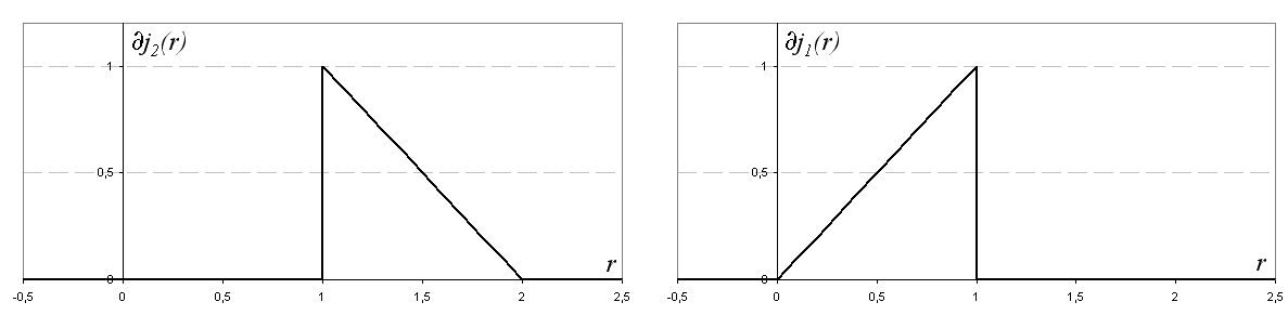
Figure 1: Examples of multifunctions used as nonmonotone and multivalued boundary conditions (46)

We consider two examples of the locally Lipschitz functionals $j$:

$$j_{1}(r)=\begin{cases}0\ \mbox{for}\ r\leq 0\\ \frac{r^{2}}{2}\ \mbox{for}\ r\in(0,1)\\ \frac{1}{2}\ \mbox{for}\ r\geq 1\end{cases}\ \ j_{2}(r)=\begin{cases}0\ \mbox{for}\ r\leq 1\\ \frac{1-(r-2)^{2}}{2}\ \mbox{for}\ r\in(1,2)\\ \frac{1}{2}\ \mbox{for}\ r\geq 2.\end{cases}$$

Their subdifferentials in the sense of Clarke are given by

$$\partial j_{1}(r)=\begin{cases}0\ \mbox{for}\ r\leq 0\ \mbox{or}\ r>1\\ r\ \mbox{for}\ r\in(0,1)\\ [0,1]\ \mbox{for}\ r=1\end{cases}\ \ \partial j_{2}(r)=\begin{cases}0\ \mbox{for}\ r<1\ \mbox{or}\ r\geq 2\\ 2-r\ \mbox{for}\ r\in(1,2)\\ [0,1]\ \mbox{for}\ r=1.\end{cases}$$ (52)

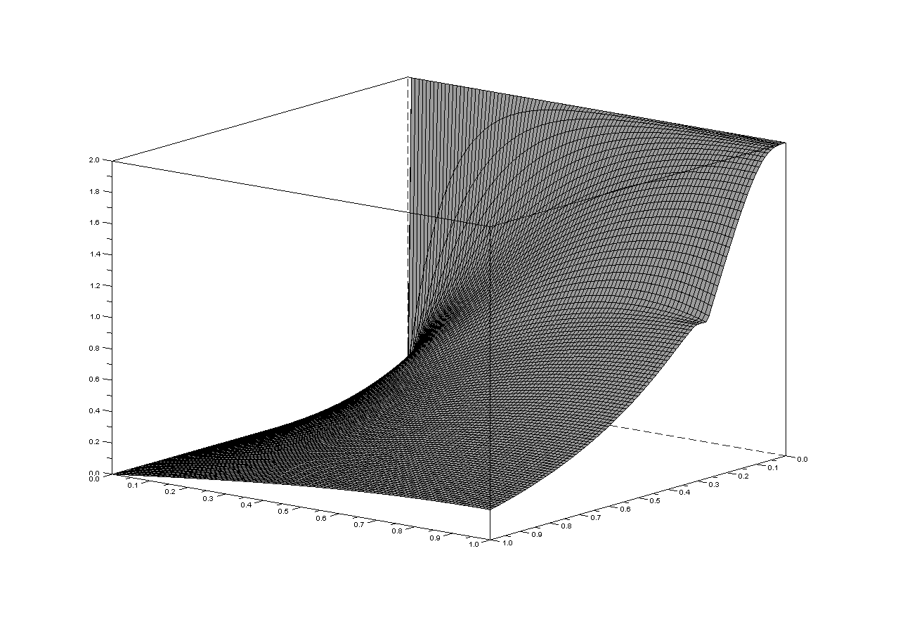
Figure 2: Simulation for the potential $j_{2}$. Plot of unique obtained solution is drawn.

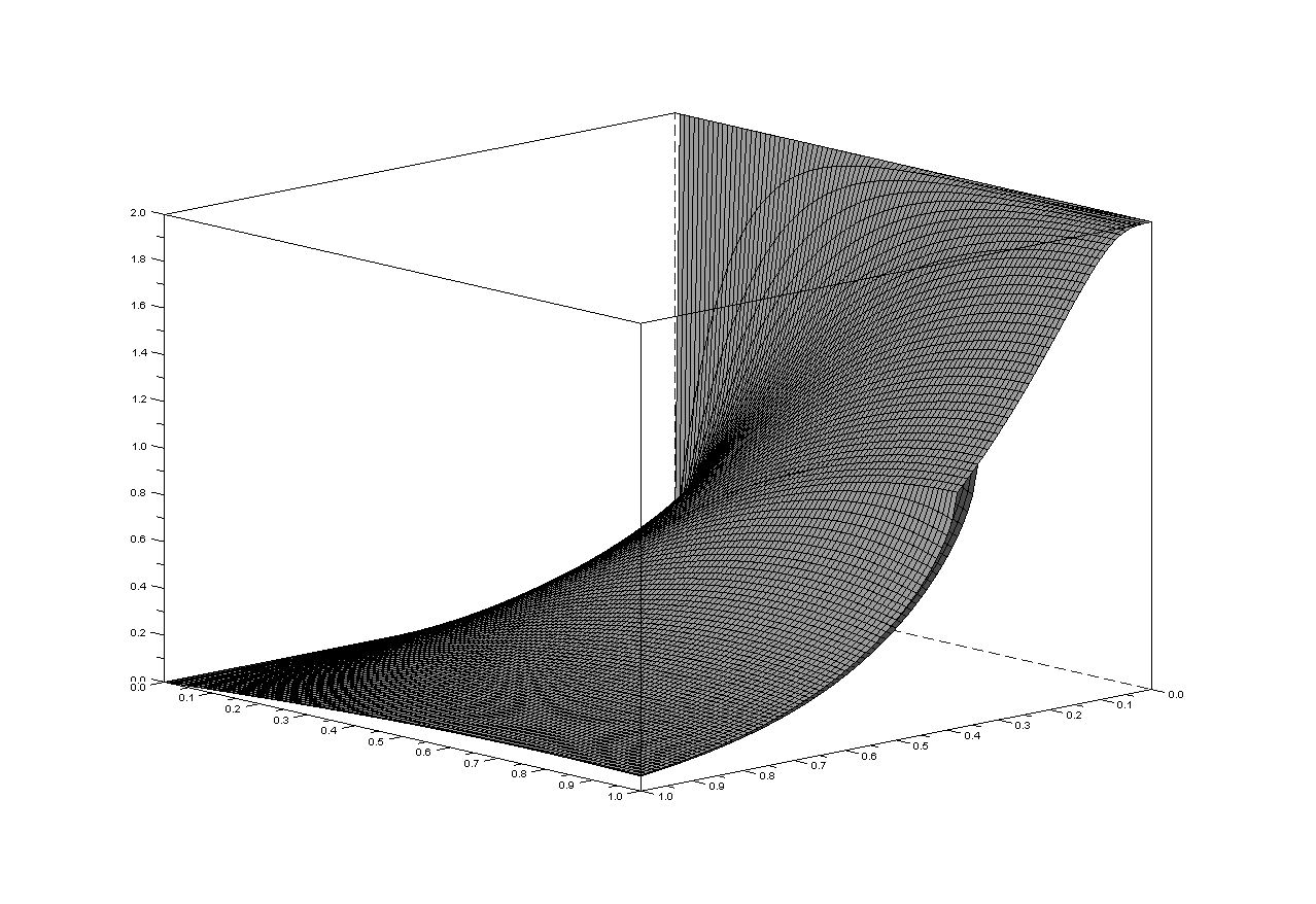
Figure 3: Simulation for the potential $j_{1}$. Plots of two (respectively maximal and minimal one) of obtained many solutions are drawn.

The graphs of $\partial j_{1}$ and $\partial j_{2}$ are presented in Figure 1. Both potentials satisfy $H(J)$. The potential $j_{1}$ does not satisfy $H(J)_{1}$ since its subdifferential has a nonmonotone jump. The potential $j_{2}$ satisfies $H(J)_{1}$ since its subdifferential has a monotone jump and nonmonotonicity is Lipschitz. In the case of $j_{1}$ the question of multiplicity of solutions remains an open problem (however the numerical simulation below show that it is more likely that there are multiple solutions) and in the case of $j_{2}$, a single solution is expected (at least as long as the inequality in $H_{const}$ holds).

In both cases we take $u_{0}(x)\equiv 2$. The following scheme is used to find solutions of (49)-(51). In every time step at most three solutions can be found:

• Assume that the element of $\partial j(\alpha_{n}^{k+1})$ for which (50) holds is equal to $0$ i.e. we fall on the horizontal line in the graph of $\partial j$. Solve the system of $n$ equations (49)-(51) and verify whether obtained $\alpha_{n}^{k+1}$ falls in the corresponding interval.

• Assume that the element of $\partial j(\alpha_{n}^{k+1})$ for which (50) holds is on the oblique line in the graph of $\partial j$. Solve the system of $n$ equations (49)-(51) and verify whether obtained $\alpha_{n}^{k+1}$ is in the corresponding interval.

• Assume that we fall on the vertical line in the graph of $\partial j$, i.e. $\alpha_{n}^{k+1}=1$. Solve the system of $n-1$ equations (49) and (51). Then verify if $\partial j(\alpha_{n}^{k+1})$ calculated from (50) falls in the interval $[0,1]$.

The simulations were run for $\Delta t=0.01$ and $\Delta x=0.01$. For the case of $j_{2}$ only one numerical solution was obtained (i.e. in every time step only one of above three cases occurred). The result is presented in Figure 2. For the case of $j_{1}$ many solutions were obtained (i.e. there were time steps in which more then one of above three cases occurred). Figure 3 shows two solutions with respectively maximum and minimum value of $\alpha_{n}^{k}$ chosen in each time step in which multiple solutions were found.

References

- [1] N.U. Ahmed, K.L. Teo, S.H. Hou, Nonlinear impulsive systems on infinite dimensions, Nonlinear Analysis, 54 (2003), 907–925.
- [2] J.P. Aubin, A. Cellina, Differential Inclusions, Springer, 1984.
- [3] J. Berkovits, V. Mustonen, Monotonicity methods for nonlinear evolution equations, Nonlinear Analysis, 27 (1996), 1397–1405.
- [4] S. Carl, Enclosure of solutions for quasilinear dynamic hemivariational inequalities, Nonlinear World, 3 (1996), 281–298.
- [5] S. Carl, R.P. Gilbert, Extremal solutions of a class of dynamic boundary hemivariational inequalities, Journal of Inequalities and Applications, 7 (2002), 479-502.
- [6] S. Carl, D. Motreanu, Extremal solutions of quasilinear parabolic inclusions with generalized Clarke s gradient, Journal of Differential Equations, 191 (2003), 206–233.
- [7] S. Carl, D. Motreanu, Extremality in solving general quasilinear parabolic inclusions, Journal of Optimization Theory and Applications, 123 (2004), 463–477.
- [8] S. Carl, Existence and comparison results for noncoercive and nonmonotone multivalued elliptic problems, Nonlinear Analysis, 65 (2006), 1532–1546.
- [9] S. Carl, V.K. Le, D. Motreanu, Evolutionary variational-hemivariational inequalities: existence and comparison results, Journal of Mathematical Analysis and Applications, 345 (2008), 545–558.
- [10] F.H. Clarke, Optimization and Nonsmooth Analysis, SIAM, Philadelphia, 1990.
- [11] Z. Denkowski, S. Migórski, N.S. Papageorgiou, An Introduction to Nonlinear Analysis, Theory, Kluwer, 2003.
- [12] Z. Denkowski, S. Migórski, N.S. Papageorgiou, An Introduction to Nonlinear Analysis, Applications, Kluwer, 2003.
- [13] J. Francu, Weakly continuous operators. Applications to differential equations, Applications of Mathematics, 39 (1994), 45–56.
- [14] D. Goeleven, D. Motreanu, Y. Dumonte, M. Rochdi, Variational and Hemivariational Inequalities: Theory, Methods and Applications, Volume II: Unilateral Problems, Kluwer, 2003.
- [15] Guanghui Wang, Xiaozong Yang, Finite difference approximation of a parabolic hemivariational inequalities arising from temperature control problem, International Journal of Numerical Analysis and Modeling, 7 (2010), 108–124.
- [16] J. Haslinger, M. Miettinen, P.D. Panagiotopoulos, Finite element method for hemivariational inequalities: theory, methods andapplications, Kluwer, 1999.
- [17] Z. Liu, S. Zhang, On the degree theory for multivalued type mappings, Applied Mathematics and Mechanics, 1 (1998), 1141–1149.
- [18] Z. Liu, A class of evolution hemivariational inequalities, Nonlinear Analysis, 36 (1999), 91–100.
- [19] Z. Liu, A class of parabolic hemivariational inequalities, Applied Mathematics and Mechanics, 21 (2000), 1045–1052.
- [20] Z. Liu, Some existence theorems for evolution hemivariational inequalities, Indian Journal of Pure and Applied Mathematics, 34 (2003), 1165–1176.
- [21] Z. Liu, Browder–Tikhonov regularization of non-coercive evolution hemivariational inequalities, Inverse Problems, 21 (2005), 13–20.
- [22] M. Miettinen, A parabolic hemivariational inequality, Nonlinear Analysis, 26 (1996), 725–734.
- [23] M. Miettinen, P.D. Panagiotopoulos, Hysteresis and hemivariational inequalities: semilinear case, Journal of Global Optimization, 13 (1998), 269- 298.
- [24] M. Miettinen, P.D. Panagiotopoulos, On parabolic hemivariational inequalities and applications, Nonlinear Analysis, 35 (1999), 885–915.
- [25] M. Miettinen, P.D. Panagiotopoulos, Hysteresis and hemivariational inequalities: quasilinear case, Applicable Analysis, 82 (2003), 535- 560.
- [26] S. Migórski, On existence of solutions for parabolic hemivariational inequalities, Journal of Computational and Applied Mathematics, 129 (2001), 77–87.
- [27] S. Migórski, A. Ochal, Boundary hemivariational inequality of parabolic type, Nonlinear Analysis, 57 (2004), 579–596.
- [28] S. Migórski, Dynamic hemivariational inequalities in contact mechanics, Nonlinear Analysis, 63 (2005), e77–e86.
- [29] Z. Naniewicz, P.D. Panagiotopoulos, Mathematical Theory of Hemivariational Inequalities and Applications, Dekker, New York, 1995.
- [30] N.S. Papageorgiou, On the existence of solutions for nonlinear parabolic problems with nonmonotone discontinuities, Journal of Mathematical Analysis and Applications, 205 (1997), 434–453.
- [31] R. Rossi, Compactness results for evolution equations, Istit. Lombardo Accad. Sci. Lett. Rend. A, 135 (2001), 19–30.
- [32] R. Rossi, G. Savare, Tightness, integral equicontinuity and compactness for evolution problems in Banach spaces, Ann. Sc. Norm. Sup., Pisa, 5 (2003), 395–431.
- [33] T. Roubiček, Nonlinear Partial Differential Equations with Applications, Birkhäuser Verlag, Basel, Boston, Berlin, 2005.
- [34] J. Simon, Compact sets in the space , Ann. Mat. Pura Appl., 146 (1987), 65–96.