HIGH CADENCE TIME-SERIES PHOTOMETRY OF V1647 ORIONIS

Abstract

We present high cadence (1–10 hr^-1) time-series photometry of the eruptive young variable star V1647 Orionis during its 2003–2004 and 2008–2009 outbursts. The 2003 light curve was obtained mid-outburst at the phase of steepest luminosity increase of the system, during which time the accretion rate of the system was presumably continuing to increase toward its maximum rate. The 2009 light curve was obtained after the system luminosity had plateaued, presumably when the rate of accretion had also plateaued. We detect a ‘flicker noise’ signature in the power spectrum of the lightcurves, which may suggest that the stellar magnetosphere continued to interact with the accretion disk during each outburst event. Only the 2003 power spectrum, however, evinces a significant signal with a period of 0.13 d. While the 0.13 d period cannot be attributed to the stellar rotation period, we show that it may plausibly be due to short-lived radial oscillations of the star, possibly caused by the surge in the accretion rate.

1 INTRODUCTION

On 9 February 2004, McNeil (2004) discovered a previously unknown object about 12 arcminutes south-west of the M78 reflection nebula. Studies of images of the area taken prior to the event confirmed that a star, V1647 Orionis, had brightened significantly over the course of a few days, illuminating the material surrounding it and creating what is now known as McNeil’s Nebula. Briceño et al. (2004), through their long-term survey of the Orion Nebula region, constrained the onset of the outburst to early November 2003. The lightcurve obtained by Acosta-Pulido et al. (2007) shows that the object reached maximum brightness by the beginning of March 2004 and had faded back to its initial state by March 2006. In examining photographic plates from the Asiago and Harvard Observatories, Aspin et al. (2006) found that this star had undergone a similar eruption in 1966, fading back to invisibility by the end of November 1967. In 2009, Aspin et al. (2009) reported that yet another outburst event began in August 2008.

The rare nature of these events in general, and the fact that we have been able to observe several of them from one star in particular, give us a unique opportunity to study such stellar outbursts within the context of star formation. Here, we present high cadence time-series photometry of V1647 Orionis from its 2003–2004 and 2008–2009 eruptions.

2 LIGHT CURVE OBSERVATIONS AND REDUCTIONS

We observed V1647 Ori during a nine-night observing run in 2003 December with the Mosaic-1 wide-field imager on the WIYN 0.9-m telescope at the Kitt Peak National Observatory. This instrument consists of eight $2048\times 4096$ pixel CCDs with a plate scale of 0$\farcs$43 pix^-1 and total field of view of 59′$\times$59′. Four of the nine nights were lost to poor weather. We used the SDSS $z$ filter at 9400Å to obtain a total of 65 images on five nights with an average cadence of $\sim$1 hr^-1. The exposure time for all images, except those taken on the first night, was 120 s. On the first night, we took shorter exposures that were 60 s as well as longer ones of 180 s. The observations were obtained at airmasses ranging from 1.8 to 2.5. This dataset samples the time during which the source’s brightness was steeply increasing (cf. Fig. 1).

We used the Y4KCam on the SMARTS 1.0-m telescope at the Cerro Tololo Inter-American Observatory to observe V1647 Ori on UT 2009 January 23. The $4064\times 4064$ CCD has a plate scale of 0$\farcs$289 pix^-1 and a field of view of 20′$\times$20′. We used the $I_{C}$ filter for our 32 images taken with an average cadence of $\sim$10 hr^-1. The exposure time for each image was 300 s and the range in airmass was 1.2 to 2.6. If we assume a rise time similar to the 2003 outburst, then these data were taken soon after the object peaked in brightness (Fig. 1).

In order to measure how the star’s brightness changed with time, we performed aperture photometry using standard IRAF routines. We used an aperture radius of 6 pixels and measured the sky background with a 5-pixel wide annulus and a 10-pixel inner radius for the 2003 data; we used an 8-pixel inner radius for the 2009 data. We selected these parameters based on the average seeing of the two datasets (3.6 pixels in 2003 and 3.0 pixels in 2009).

We performed differential photometry because the observing conditions were non-photometric in both 2003 and 2009. Because most of the stars in this field are likely variable, we did not attempt to choose a single comparison star with which to determine the differential light curve of V1647 Ori. We expect that on average any variations in the field stars are uncorrelated except for effects of the instrument and sky conditions. Thus we selected five calibration stars (Table 1) in the vicinity of the McNeil’s object that were of comparable brightness to V1647 Ori with which we defined an average “reference star.” We checked that none of these are known to be variables. We further checked that the differential light curve of each of these stars, determined relative to the other four calibration stars, was not variable within the photometric errors.

The full differential light curve from 2003 December is presented in Table 2 and from 2009 January in Table 3. The errors on individual photometric measurements are typically 0.02 mag in the 2003 data and 0.01 mag in the 2009 data, which include both the formal photometric errors of V1647 Ori and the error of the mean of the combination of the five comparison stars.

3 RESULTS

3.1 2003 light curve

3.1.1 Variability

Our data show that V1647 Ori brightened by almost 2 mag over the course of our 9-night run in 2003 December (Fig. 2, top). This steep rise in brightness is approximately linear (in magnitudes), but with low-level structure superposed on top of the linear trend. To explore the structure of these low-level brightness variations, we de-trended the light curve as follows.

First we subtracted a linear fit (Fig. 2, top, dashed line), which reveals a slow brightness variation with a peak-to-peak amplitude of $\sim$0.3 mag (Fig. 2, middle). These variations are reminiscent of those commonly observed in classical T Tauri stars, which can arise from variations in the accretion stream or from modulation due to star spots at the stellar rotation period, and which often exhibit periodic or quasi-periodic behavior (Type IIp and Type II, respectively, in the nomenclature of Herbst et al., 1994) on timescales of $\sim$1–10 d. The V1647 Ori variations appear to modulate on a timescale of 4–5 d. We cannot establish with our data whether this signal is strictly periodic because our light curve spans only two cycles of such a period, and moreover the data gaps in the light curve leave large phase gaps when the light curve is folded on such a period. Furthermore, we show below that this light curve modulation cannot be the rotation period of the star. In the following we refer to this component of the light curve variability as a “quasi-periodic” modulation. We defer speculation about its possible physical significance to Sec. 4.

Next we further de-trended the light curve by subtracting a best-fit sinusoid as a simple representation of the quasi-periodic modulation ($P$=4.14 d; Fig. 2, middle, dashed curve). The resulting residual light curve (Fig. 2, bottom) reveals very short-timescale variations that are significantly larger than the noise in our data (reduced chi-square is $\chi^{2}_{\nu}=9.7$). The amplitude of these variations is $\sigma_{\rm rms}\approx 0.05$ mag.

We conducted a few simple tests to verify that none of the periodic photometric signals discussed here and in what follows correlate with seeing variations. We performed aperture photometry on a portion of the nebula itself using, as before, a 6 pixel aperture radius; we separately performed aperture photometry on V1647 Ori using a larger (9 pixel) aperture radius. We executed a periodogram analysis (as below) on the resultant light curves and also on the seeing variations, which were obtained by measuring the average FWHM of our calibration stars in each image. We found no significant differences in the target light curve, and no evidence for significant periodicities in either the nebular light curve or in the seeing variations (and in particular not at the periods reported below). We conclude that changes in seeing are not driving the periodic photometric variations we report in this work.

3.1.2 Periodogram analysis

To examine the light-curve variations of V1647 Ori in detail, we subjected the 2003 light curve (Fig. 2) to a standard Lomb-Scargle power spectrum analysis. The Lomb-Scargle periodogram is well-suited to unevenly sampled data such as ours. It moreover possesses well characterized statistical properties that permit quantitative assessment of the statistical significance of any periodic behavior in the data (see Press et al., 1992, and references therein). We will exploit these statistical properties below.

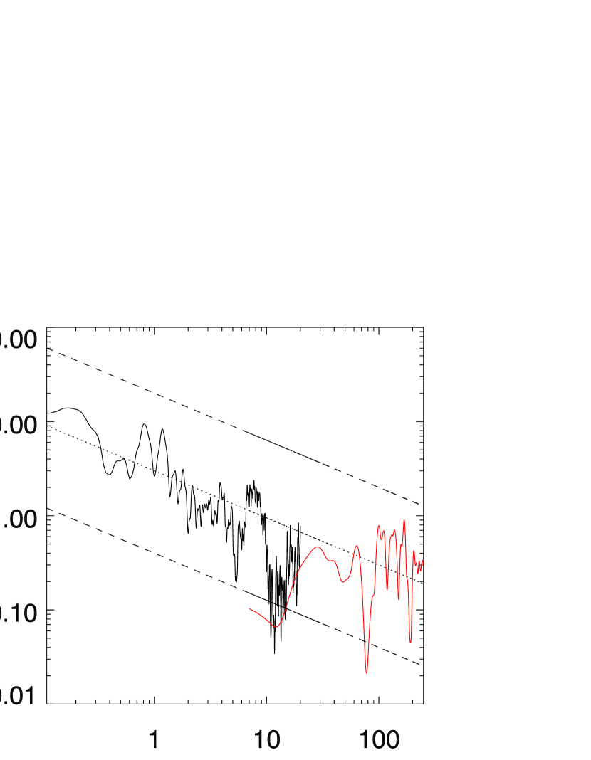
Figure 3: Power spectrum resulting from a Lomb-Scargle periodogram analysis of the non-detrended light curve of V1647 Ori, on a log-log scale. The frequency range $0.1<f<18$ d^-1 (black) is provided by the 2003 light curve data (Fig. 2, top), whereas the frequency range $7<f<135$ d^-1 (red) is provided by the high-cadence 2009 light curve data (Fig. 6). Following the usual definition of the Lomb-Scargle periodogram, the ordinate gives the spectral power normalized by the variance of the data. The power spectrum overall follows a slope of $1/\sqrt{f}$ (dashed/dotted lines), and in addition exhibits peaks near frequencies of $\sim$ 0.2, 0.8, 1.2, and 8 d^-1 (see the text for discussion of the meaning of these peaks).

Fig. 3 shows the power spectrum of the non-detrended light curve (Fig. 2, top) over the frequency range 0.1–18 d^-1. The low frequency cutoff corresponds to $1/T$ where $T$ is the total timespan of the data while the high frequency cutoff corresponds to half the sampling frequency (i.e., the Nyquist limit). Overall the power spectrum rises toward smaller frequencies, with a slope that closely approximates a $1/\sqrt{f}$ dependence (represented by dashed/dotted lines in the figure). In addition, the power spectrum exhibits several peaks on top of the $1/\sqrt{f}$ slope. The broad peak at $f\sim 0.2$ d^-1 corresponds to the slow, quasi-periodic modulation discussed in Sec. 3.1.1 (see also Fig. 2, middle). The two peaks near $f=0.8$ d^-1 and $f=1.2$ d^-1 are aliases of the $f\sim 0.2$ d^-1 modulation beating against the diurnal data gaps ($f=1$ d^-1). The peak near $f=8$ d^-1 is due to the short-timescale variability in the detrended light curve (Fig. 2 bottom).

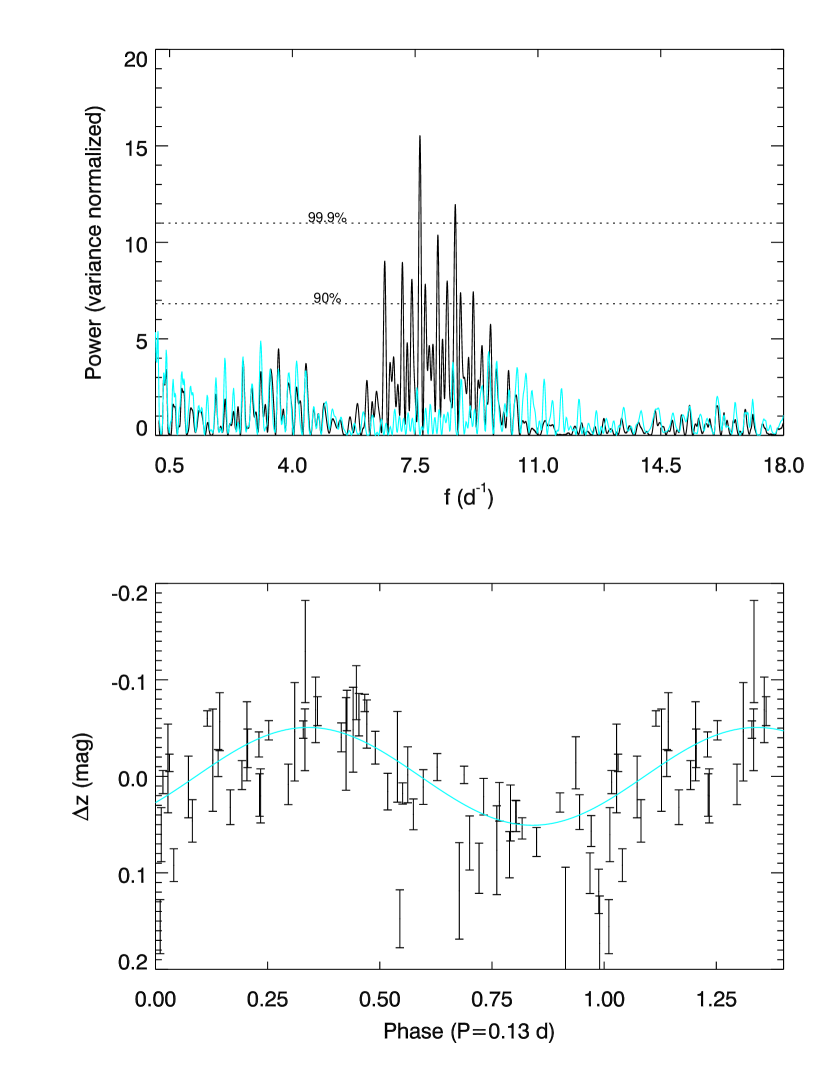
Figure 4: Top: Power spectrum of the detrended light curve from Fig. 2c (black). The highest peak is at 7.7 d^-1 (a period of 0.13 d). Dotted lines represent the peak heights corresponding to confidence levels of 90% and 99.9%; a peak above the 99.9% confidence line, for example, would have a false-alarm probability (FAP) lower than 0.1%. The signal at 0.13 d, is very highly statistically significant, with a FAP of $1.3\times 10^{-5}$. (See the text and Fig. 5 for FAP details.) The blue curve shows the result of removing the 0.13 d period; no significant periods remain. Bottom: Light curve data are phased on the 0.13 d period with best-fit sinusoid in blue. The amplitude of the sinusoid is 0.051 mag.

The power spectrum of the detrended light curve is shown in Fig. 4 (top, black curve). Not surprisingly, nearly all of the power at low frequencies has been eliminated by the de-trending of the linear rise and of the slowly varying quasi-periodic modulation. The power spectrum shows a strong peak at 7.7 d^-1, corresponding to a period of 0.13 d, and several other strong features at nearby frequencies, which have power levels corresponding to a statistical confidence of 90% or higher (see below). When we filter out the 0.13-d period peak by subtracting the best fitting sinusoid from the light curve, all of the other statistically significant peaks in the periodogram are also removed (Fig. 4, top, blue curve), showing them to be aliases and beats of the 0.13 d period. The light curve (Fig. 2, bottom) is shown folded on this period in Fig. 4 (bottom), with the best-fitting sinusoid overlaid in blue. The amplitude of this sinusoid is 0.051 mag.

To empirically determine the false-alarm probability (FAP) corresponding to different power levels in the periodogram, we used a Monte Carlo bootstrapping technique as described in Press et al. (1992) and implemented in e.g. Stassun et al. (1999, 2002). We generated 10,000 artificial light curves by shuffling the actual measurements in temporal order and sampling at the same timestamps as the actual data. In this way, the artificial light curves retain both the noise properties and the time windowing of the real data. For each of the 10,000 artificial light curves, we calculated a power spectrum as for the real data and recorded the power level of the strongest peak in each. The resulting distribution of these 10,000 maximum peak heights gives directly the probability of a given peak height occurring by chance.

The distribution of maximum peak heights is shown in Fig. 5 for 10,000 artificial light curves simulating the detrended 2003 light curve (Fig. 2, bottom). From the figure, peak heights with power levels above $\sim$7 occur in fewer than 10% of the simulated power spectra, whereas peaks with power levels above $\sim$11 occur in fewer than 0.1% of the simulated power spectra; these then define the 10% and 0.1% FAP levels, respectively (or equivalently, the 90% and 99.9% confidence levels). These confidence levels are represented by horizontal dotted lines in the observed power spectrum (Fig. 4, top).

As described by Press et al. (1992), the FAP for a given peak height in a Lomb-Scargle periodogram is expected to follow an analytic relationship (cf. their Eq. 13.8.7) shown in Fig. 5 as a dotted curve. Evidently, our data and its associated power spectrum closely follow the expected statistical behavior. Fig. 5 shows the FAP calculation for the 0.13 d period. The observed peak height (shown as vertical dashed line) has a FAP of $1.3\times 10^{-5}$, and is therefore very highly statistically significant.

We checked that the 0.13 d period and its statistical significance are not dependent on the details of the sinusoidal de-trending that we performed in Sec. 3.1.1. As a simple alternative to the sinusoidal detrending (see Fig. 2, middle), we instead simply shifted all of the data points from a given night such that the mean differential $z$ magnitude for the observations made on each night was 0.0. We then performed the same periodogram analysis as above. We recovered the same 0.13 d period as before with a FAP of $3.6\times 10^{-5}$, again highly statistically significant.

3.1.3 Stellar Rotation

Since periodic signals in young, low-mass stars are often associated with rotation, we explored the possibility that we have detected stellar rotation in our light curve. The rotation periods of low-mass pre–main-sequence stars are most typically in the range $\sim$2–10 d (e.g., Herbst et al., 2002), though some young low-mass stars have been observed to rotate with periods as short as $\sim 0.1$ d (Stassun et al., 1999).

Adopting values for the visual extinction ($19\pm 2$ mag), K-band veiling ($1.5\pm 0.2$ mag), spectral type ($M0\pm 2$ subclasses), and K-band apparent magnitude (9.9 mag in February 2007) as determined by Aspin et al. (2008), a bolometric correction of $BC_{V}=-1.3$ and a $(V-K)$ color of 3.7 as appropriate for an M0 spectral type (Kenyon & Hartmann, 1995), the equations for absolute $K$ magnitude and bolometric luminosity from Greene & Lada (1997), and a distance of $426\pm 20$ pc (Menten et al., 2007; Kraus et al., 2007; Hirota et al., 2007), we calculate a stellar radius of $4.2^{+1.0}_{-1.3}$ R_⊙.

Aspin et al. (2009) observed line broadening in the spectrum of V1647 Ori of 120 km s^-1. While the spectra of EXor and FUor eruptive variables can be dominated by the hot “atmosphere” of the inner accretion disk during outburst, the Aspin et al. (2009) observations were obtained during quiescence of the system; we therefore presume that the observed spectral broadening is stellar in origin. This then provides a lower limit on the stellar rotational velocity of $v\sin i$=120 km s^-1. We can also assume an upper limit from break-up considerations of $v_{\rm rot}$$\approx$190 km s^-1.

With these upper and lower bounds on the rotational velocity of V1647 Ori, if we simultaneously push all other measured parameters to their 1 $\sigma$ limits so as to produce the shortest and longest possible rotation periods, we find with greater than 99.9% confidence that the stellar rotation period lies between 0.6 and 2.7 days. To test the robustness of our calculations, we also calculated the stellar radius using the quiescent V-band extinction and K-band apparent magnitude obtained by Ábrahám et al. (2004) prior to the 2004 outburst ($\sim$13 and 10.3 magnitudes, respectively); from this, and assuming an inclination angle of $61^{\circ}\pm 14^{\circ}$ as found by Acosta-Pulido et al. (2007), we obtain a most likely rotation period of $\sim$1 d, consistent with the above range. If this is indeed the rotational period of the star, the diurnal gaps in our lightcurve would preclude its detection. In any case, we conclude that the 0.13 d period, and the $\sim$4 d quasi-periodic modulation, do not correspond to the rotation period of V1647 Ori.

3.2 2009 light curve

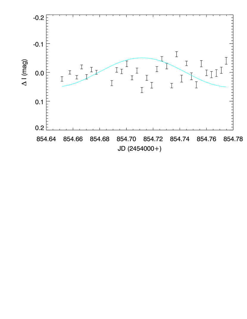
Figure 6: Lightcurve of V1647 Ori during 2008–2009 outburst, spanning 0.13 d. These data were taken after the object had reached maximum brightness. No obvious periodic brightness variations are evident. The best-fit 0.13 d sinusoid observed in the 2003 outburst data (Fig. 4b) is overplotted here for comparison.

Figure 6 displays our 2009 light curve. The dataset was obtained at very high cadence ($\sim 10$ hr^-1) over a timespan of several hours on a single night and, thus, is sensitive only to high frequency variations. A simple $\chi^{2}$ test shows the light curve to be variable, with reduced $\chi_{\nu}^{2}=10.0$. However, applying the same periodicity analysis as above, we find no significant periodicity in this light curve across the frequency range to which we are sensitive, from 7 d^-1 to 135 d^-1; the strongest peak we obtain has a FAP of 41%.

The full duration of the 2009 light curve is (coincidentally) 0.13 d (7.7 d^-1), and thus can be used to check for the presence of a 0.13 d period during the 2009 observations. As shown in Fig. 6, a 0.13 d period such as that observed in the 2003 light curve (Fig. 4b) is not present in the 2009 light curve. As an additional check, we injected a 0.13 d sinusoid of varying amplitude into these data and found that we were able to induce a significant peak in the power spectrum (FAP $<$ 1%) only if the amplitude of the sinusoid is larger than 0.027 mag. We thus conclude that there is no evidence for an 0.13 d period in the 2009 data with an amplitude greater than 0.027 mag, and we can definitively rule out an 0.13 d signal with an amplitude of 0.05 mag as seen in the 2003–2004 outburst light curve (Fig. 2). To summarize, we find that this 2009 lightcurve is variable, but no periodic phenomenon with a frequency in the range to which we are sensitive (7 d^-1 to 135 d^-1) is driving this variability.

In Fig. 3 we show the power spectrum of the 2009 light curve data together with that from the 2003 data. The two datasets sample a mostly disjoint range of temporal frequencies. However, the two power spectra together are consistent with a single $1/\sqrt{f}$ behavior for the power spectrum as a whole. We suggest one possible interpretation for this $1/\sqrt{f}$ behavior below (Sec. 4.2). The only clearly evident difference between the 2003 and 2009 power spectra is in the overlap region near $f=10$ d^-1; as discussed above the 2003 light curve exhibits a strong 0.13 d period whereas the 2009 light curve does not.

4 DISCUSSION

We have found strong evidence to suggest that V1647 Ori exhibited a highly significant 0.13 d periodicity in brightness during the rapid brightening phase of its 2003 outburst. The amplitude of this periodic variation was $\sim$0.05 mag. The presence of this feature in the 2003 data, obtained while the object was in the brightening phase, and its absence in the 2009 data, obtained after V1647 Ori had peaked in brightness, suggest that this phenomenon, whatever its cause, is associated with the unstable period of time when the brightness of V1647 Ori was most rapidly increasing. We have also found evidence for a $1/\sqrt{f}$ slope in the power spectrum of V1647 Ori over a large range of temporal frequencies, $0.1<f<135$ d^-1.

In this section, we consider whether the 0.13 d period may be ascribed to short-lived stellar pulsations, perhaps triggered by the high accretion event. Next, we discuss “flickering” in the light curve, evidenced by the $1/\sqrt{f}$ slope in the power spectrum, in the context of a magnetically channeled accretion flow. Finally, we consider whether oscillations originating in the accretion disk, similar to those observed during cataclysmic variable (CV) star outbursts, could be observed in young star outbursts, including FUor and EXor events, and we speculate that the $\sim$4 d quasi-periodic modulation observed in the 2003 light curve could correspond to such an oscillation. The consideration of these mechanisms here is speculative; our aim is to examine whether these explanations may be plausible, but we cannot yet establish that these are definitive driving mechanisms for the observed variability.

4.1 Stellar pulsations

Since it is inconsistent with the likely rotation period of V1647 Ori (Sec. 3.1.3), we explore the possibility that the 0.13 d period might be a manifestation of pulsation. Given its effective temperature and estimated mass of $0.8\pm 0.2$ M_⊙ (Aspin et al., 2008), and based on comparison with stellar evolutionary tracks (D’Antona & Mazzitelli, 1994), we find that V1647 Ori may lie just within the theoretically predicted deuterium instability strip. The expected fundamental mode pulsation period would be approximately 0.5 d (e.g., Toma, 1972), somewhat longer than the period we detect. In addition, the 0.13 d period does not appear in the 2009 data. It is extremely unlikely that V1647 Ori transitioned from being within the instability strip to being outside the instability strip between our 2003 and 2009 observations.

We next consider whether the dramatic increase in the accretion rate could have induced short term radial oscillations of the stellar surface. From the idealized homogeneous compressible model presented by Cox (1980), the period of oscillation, for purely radial pulsation, varies according to

$$\frac{4\pi^{2}R^{3}}{P^{2}GM}=-4+\Gamma_{1}(2n^{2}+5n+3)$$ (1)

where $R$ is the star’s radius, $P$ is its pulsational period, $G$ is the gravitational constant, $M$ is the stellar mass, $\Gamma_{1}$ the adiabatic exponent, and $n$ the pulsational mode. For our purposes here, this idealized model is not significantly different from more sophisticated models (Tassoul and Tassoul, 1968). Adopting the stellar parameters of V1647 Ori (see Sec. 3.1.3) and assuming as one extreme assumption that no part of the star is ionized ($\Gamma_{1}=\frac{5}{3}$), we find that the 0.13 d period could correspond to pulsational modes ranging from 2.8 to 4.7. In order to determine the effect of ionization zones on our results, we looked at the extreme case of a fully ionized gas ($\Gamma_{1}=\frac{4}{3}$); in this case we find pulsational modes between 3.3 and 5.4. Hence, any errors in not taking ionization zones into account do not significantly change our results. We therefore infer that the 0.13 d period most likely corresponds to a radial pulsation in the $4^{th}$ oscillation mode, but the $3^{rd}$ and $5^{th}$ modes are also permitted within the observational uncertainties in the stellar properties of V1647 Ori.

Pulsation solely in a higher overtone radial mode, although rare, is strongly dependent on the location of the driving mechanism (Kurtz, 2006). Examples of similar short-term oscillation-producing phenomena include recent solar observations (Karoff & Kjeldsen, 2008) that revealed that energetic magnetic reconnection and coronal mass ejection events can induce short-lived high-frequency oscillations of the solar surface. In the Sun, these are confined to the vicinity of the triggering event (e.g., Kienreich et al., 2009). The triggering of radial oscillations by the sudden onset of highly energetic accretion on V1647 Ori thus provides one possible explanation for the observed variability.

4.2 Flickering

Flickering is defined as random, small amplitude brightness variations recurring on dynamical timescales (Kenyon et al., 2000). Sometimes interpreted as an observable consequence of an inhomogeneous accretion flow, flickering has been observed in CV stars and, as it is associated with accretion, could be observable during similar outburst events in young stars. Indeed, Kenyon et al. (2000) and Rucinski et al. (2008) observed flickering in the lightcurves of FU Ori and TW Hya, respectively, the latter through observation of a $1/\sqrt{f}$ slope in the power spectrum. The combination of a high observing cadence and a relatively long time baseline means that our data are sensitive to a large range of frequencies, and, as such, any signs of this phenomenon should be readily apparent in an analysis of the power spectrum of our data.

As discussed in Sec. 3, the overall power spectrum of the observed phases of the 2003–2004 and 2008–2009 outbursts of V1647 Ori follow a $1/\sqrt{f}$ trend (Fig. 3), which suggests that flickering is one possible origin of the random variability components of the light curve.

The nature of such “flicker noise” is not entirely understood; however, it appears to be linked to situations in which a flow (in this case the accretion of material from disk to star) is funneled or is in some way forced to pass through a physically confined region (Press, 1978). Indeed, accretion in young low-mass stars is typically envisioned to occur via magnetospheric funneling of disk material along stellar field lines that thread the inner accretion disk (e.g. Shu et al., 1994). Also, the flickering observed in the CV system T CrB, for example, has been attributed to turbulence in the inner regions of the accretion disk (Dobrotka et al., 2010). Thus the observation of flickering in V1647 Ori might suggest an interaction between the stellar magnetosphere and the inner regions of the accretion disk during outburst, with material continuing to accrete onto the star along stellar magnetic field lines (e.g. Shu et al., 1994).

4.3 Dwarf Nova-Like Oscillations in the Keplerian Inner Accretion Disk?

We have observed a modulation with a timescale of $\sim$4 d in the 2003 light curve of V1647 Ori (Fig. 2). As discussed, our data do not permit us to determine whether this modulation is strictly periodic, or indeed whether it persists for more than $\sim$2 cycles. It is nonetheless a potentially interesting quasi-period that could arise in a number of different ways.

Dwarf-nova oscillations (DNOs) are quasi-periodic brightness variations typically observed in cataclysmic variable star outbursts. These phenomena are associated with accretion, and they may persist during quiescence (Pretorius et al., 2006). The oscillations are not observed in all CV outbursts, and the oscillation frequencies may change during a high-accretion event. Because of their relatively short periods, DNOs are believed to originate at the inner edges of Keplerian accretion disks. They have only rarely been observed during the rise of a CV outburst (Warner & Pretorius, 2008), but their behavior is thought to be well described by a low-inertia magnetic accretor model in which accretion induces variations in the angular velocity of an equatorial accretion belt (Warner & Woudt, 2002). In addition, so-called quasi-periodic oscillations (QPOs), which are longer term, less coherent oscillations, have also been observed during some CV outbursts. There is no generally accepted model for what causes the QPO brightness modulations, but they are thought to be accretion disk phenomena (e.g., Woudt & Warner, 2002). In any event, an empirical relationship links DNOs to QPOs such that $P_{\rm QPO}\approx 15\times P_{\rm DNO}$ (Warner & Woudt, 2002).

The low-inertia magnetic accretor model predicts that the DNO oscillation quasi-period ($P_{\rm DNO}$) increases as the accretion rate ($\dot{M}$) decreases. It also predicts that $P_{\rm DNO}$ corresponds to the Keplerian orbital period of the inner edge of the accretion disk. If we assume a $P_{\rm DNO}$–$\dot{M}$ relation such as that found empirically for the dwarf nova SS Cyg by Mauche (1997) and use the $\dot{M}$ found for V1647 Ori by Muzerolle et al. (2005), we find $P_{\rm DNO}\sim 5.7$ d. We note that the value of $\dot{M}$ might differ for our data, bringing $P_{\rm DNO}$ closer to our observed quasi-period of 4.14 d. For example, using the $P_{\rm DNO}$–$\dot{M}$ relation, we calculate that $\dot{M}\sim 10^{-4}$ M_⊙ yr^-1 would yield a period of 4.2 d. In any event, if this model applies to the V1647 Ori system, then, taking the mass of the central star to be $\sim 0.8~{}$M_⊙, we calculate that the inner edge of the accretion disk surrounding V1647 Ori was located $\sim$2.5 stellar radii from the star prior to the peak of the outburst. This model could thus suggest that the stellar magnetosphere was still capable of holding off the inner disk, at least during the early stages of the 2003–2004 outburst.

Additionally, using the relation of $P_{\rm QPO}\approx 15\times P_{\rm DNO}$, we would expect to observe a QPO with a period of $\sim$60 d, which is very close to the 56 d period found by Acosta-Pulido et al. (2007) who attributed it to dense circumstellar clumps orbiting the star. However, given the non-uniform sampling of our data and the fact that these oscillations are observed over only $\sim$2 cycles, the reality of this period, and the link between these periodicities and those observed in white dwarf stars, is unclear. Nevertheless, they are potentially intriguing. Observations probing similar timescales during FUor/EXor outbursts would allow us to further investigate the presence of such phenomena in young star outbursts.

5 SUMMARY

In this work, we present high cadence time-series photometry of V1647 Orionis during its two most recent outburst events. The overall power spectrum of our 2003 and 2009 datasets displays a $1/\sqrt{f}$ ‘flicker noise’ spectrum. The detection of ‘flicker noise’ in the power spectra of our light curves suggests that accretion continues to be mediated by the stellar magnetosphere during the observed phases of the 2003–2004 and 2008–2009 outbursts. This picture is bolstered by the observation of a quasi-periodic modulation in the 2003 light curve with a timescale of $\sim$4 d, perhaps arising from a CV-like quasi-periodic oscillation of the inner accretion disk edge at a height of 2–3 stellar radii from the stellar surface.

Our Fourier analysis of our 2003 detrended lightcurve, obtained mid-outburst, yields a periodic variation on a timescale of 0.13 d that persists in spite of the dramatic rise in brightness caused by the outburst. This period, detected at very high statistical significance, is not attributable to the expected rotation period calculated from other measured properties of the star. This 0.13 d period is absent from our 2009 light curve.

The 0.13 d period is very coherent in the 2003 dataset, and it is therefore likely to have been a truly periodic phenomenon during those observations. Given that we do not detect this period in our 2009 light curve, obtained post-outburst, we conclude that it is probably an accretion-induced process associated with the epoch when the brightness of the object is increasing (and so perhaps when the accretion rate is increasing), one likely candidate being short-lived radial pulsations of the star.

Figure 1: Our datasets in context. The 2003 data were taken in 2003 December, during the phase of steepest increase in brightness. No outburst lightcurve has yet been published for the 2008-2009 event, but if we assume a rise-time similar to the 2003-2004 outburst, our 2009 data would sample the phase when the brightness of V1647 Ori had plateaued, as shown. Adapted from Acosta-Pulido et al. (2007).

Figure 2: (Top): Differential light curve of V1647 Ori obtained mid-outburst in 2003 December. The system brightened by $\sim 2$ mag over the course of 9 nights. For reference, the dotted line represents a linear trend fit to the data. The scale of the time axis has been chosen to allow direct comparison with the long-term light curve data presented in Briceño et al. (2004, cf. their Fig. 3). (Middle): Same light curve de-trended with the linear trend from top, revealing a quasi-periodic modulation with a timescale of $\sim$4 d. For reference, the dotted curve represents a sinusoidal trend fit to the data ($P$=4.14 d). (Bottom): Same light curve further de-trended with the sinusoidal trend from middle, revealing short-timescale variations with amplitude $\sim$0.05 mag.

Figure 5: The false alarm probability (FAP) of the 0.13 d period as a function of peak height as determined from Monte Carlo simulations. The solid line represents the probability determined from our data, and the dotted curve, which nearly overlays the solid line, shows the analytical probability described by Press et al. (1992). The vertical dashed line shows the peak height we actually observe in Fig. 4a. The FAP of the 0.13 d period is $1.3\times 10^{-5}$.

Table 1: J2000 coordinates of stars used for differential photometry

RA	Dec
05:46:22	-00:03:37
05:46:29	-00:03:47
05:46:31	-00:04:21
05:46:28	-00:09:59
05:46:26	-00:10:25

Table 2: Differential photometric measurements of V1647 Ori in 2003 December

JD	$\Delta z$	$\sigma_{\rm mag}$
2978.7040	0.000	0.046
2978.7100	0.020	0.032
2978.7410	-0.034	0.051
2978.7440	-0.026	0.032
2978.7560	-0.020	0.048
2978.7590	-0.073	0.028
2978.7710	-0.005	0.047
2978.7740	0.014	0.029
2978.8000	0.095	0.046
2978.8040	0.056	0.029
2978.8300	0.194	0.049
2978.8330	0.082	0.028
2978.8580	-0.012	0.041
2978.8620	0.045	0.028
2978.8890	-0.021	0.044
2978.8930	-0.026	0.025
2978.9200	0.150	0.050
2978.9230	0.101	0.028
2978.9510	0.182	0.053
2978.9540	0.021	0.027
2978.9790	0.021	0.053
2978.9810	-0.019	0.030
2979.0060	-0.089	0.053
2979.0090	-0.028	0.034
2982.7000	-0.661	0.030
2982.7320	-0.725	0.024
2982.7610	-0.648	0.028
2982.7900	-0.782	0.022
2982.8190	-0.863	0.022
2982.8600	-0.769	0.020
2982.8890	-0.673	0.023
2982.9850	-0.687	0.026
2983.6870	-0.690	0.022
2983.7150	-0.729	0.021
2983.7440	-0.723	0.019
2983.7720	-0.719	0.019
2983.8000	-0.705	0.018
2983.8290	-0.713	0.018
2983.9340	-0.656	0.021
2983.9650	-0.790	0.020
2983.9940	-0.833	0.021
2984.6570	-0.998	0.017
2984.6710	-0.963	0.018
2984.7200	-0.939	0.016
2984.7490	-1.011	0.015
2984.7780	-1.063	0.015
2984.8060	-1.045	0.014
2984.8350	-0.981	0.015
2984.8730	-1.081	0.014
2984.9020	-1.149	0.015
2984.9300	-1.056	0.016
2984.9600	-1.068	0.016
2984.9910	-1.033	0.017
2986.6640	-1.569	0.011
2986.6920	-1.636	0.009
2986.7210	-1.668	0.010
2986.7490	-1.695	0.009
2986.7780	-1.619	0.009
2986.8060	-1.589	0.010
2986.8340	-1.674	0.008
2986.8620	-1.661	0.009
2986.8910	-1.592	0.011
2986.9240	-1.570	0.012
2986.9520	-1.599	0.012
2986.9800	-1.635	0.013

Table 3: Differential photometric measurements of V1647 Ori in 2009 January

JD	$\Delta I$	$\sigma_{\rm mag}$
4854.6518	0.023	0.008
4854.6576	0.000	0.006
4854.6628	0.017	0.006
4854.6665	-0.019	0.007
4854.6702	0.015	0.008
4854.6739	-0.010	0.008
4854.6776	-0.000	0.007
4854.6854	0.000	0.009
4854.6891	0.037	0.009
4854.6927	-0.009	0.008
4854.6964	-0.003	0.008
4854.7003	-0.030	0.010
4854.7042	0.019	0.007
4854.7079	-0.006	0.009
4854.7116	0.061	0.009
4854.7153	0.019	0.009
4854.7190	0.045	0.010
4854.7229	-0.011	0.009
4854.7266	-0.047	0.008
4854.7302	-0.022	0.010
4854.7339	0.046	0.008
4854.7376	-0.063	0.009
4854.7414	0.022	0.012
4854.7451	-0.031	0.008
4854.7487	0.013	0.012
4854.7524	0.043	0.011
4854.7561	-0.030	0.011
4854.7601	0.002	0.010
4854.7637	0.008	0.011
4854.7674	0.002	0.012
4854.7711	-0.007	0.011
4854.7748	-0.040	0.012

References

- Ábrahám et al. (2004) Ábrahám, P., Kóspál, Á., Csizmadia, Sz., Moór, A., Kun, M., Stringfellow, G. 2004, A&A, 419, 39
- Acosta-Pulido et al. (2007) Acosta-Pulido, J. A., et al. 2007, AJ, 133, 2020
- Aspin et al. (2006) Aspin, C., Barbieri, C., Boschi, F., Di Mille, F., Rampazzi, F., Reipurth, B., & Tsvetkov, M. 2006, AJ, 132, 1298
- Aspin et al. (2008) Aspin, C., Beck, T., & Reipurth, B. 2008, AJ, 135, 423
- Aspin et al. (2009) Aspin, C., Greene, T., & Reipurth, B. 2009, AJ, 137, 2968
- Briceño et al. (2004) Briceno, C., et al. 2004, ApJ, 606, L123
- Cox (1980) Cox, J. P. 1980, Theory of Stellar Pulsation, Princeton University Press, Princeton, New Jersey
- D’Antona & Mazzitelli (1994) D’Antona, F. & Mazzitelli, I. 1994, ApJS, 90, 467
- Dobrotka et al. (2010) Dobrotka, A., et al. 2010, MNRAS, 402, 2567
- Greene & Lada (1997) Greene, T. & Lada, C. 1997, AJ, 114, 2157
- Herbst et al. (2002) Herbst, W., Bailer-Jones, C. A. L., Mundt, R., Meisenheimer, K., & Wackermann, R. 2002, A&A, 396, 513
- Herbst & Wittenmyer (1996) Herbst, W., & Wittenmyer, R. 1996, BAAS, 189, no.4908
- Herbst et al. (1994) Herbst, W., Herbst, D. K., Grossman, E. J., & Weinstein, D. 1994, AJ, 108, 1906
- Hirota et al. (2007) Hirota, T., et al. 2007, PASJ, 59, 897
- Karoff & Kjeldsen (2008) Karoff, C., & Kjeldsen, H. 2008, ApJ, 678, L73
- Kenyon & Hartmann (1995) Kenyon, S. & Hartmann, L. 1995, ApJS, 101, 117
- Kenyon et al. (2000) Kenyon, S., Kolotilov, E. A., Ibragimov, M. A., & Mattei, J. A. 2000, ApJ, 531, 1028
- Kienreich et al. (2009) Kienreich, I. W., Temmer, M., & Veronig, A. M. 2009, ApJ, 703, L118
- Kraus et al. (2007) Kraus, S., et al. 2007, A&A, 466, 649
- Kurtz (2006) Kurtz, D. W., 2006, in ASP Conf. Ser., Astrophysics of Variable Stars, eds., C. Sterken & C. Aerts, 347, 101
- Mauche (1997) Mauche, C. 1997, in ASP Conf. Ser., Accretion Phenomena and Related Outflows, ed., D. T. Wickramasinghe, L. Ferrario, & G. V. Bicknell, 121, 251
- McNeil (2004) McNeil, J. 2004, IAU Circ. 8284
- Muzerolle et al. (2005) Muzerolle, J., Megeath, S. T., Flaherty, K. M., Gordon, K. D., Rieke, G. H., Young, E. T., & Lada, C. J. 2005, ApJ, 620, L107
- Menten et al. (2007) Menten, K. M., Reid, M. J., Forbrich, J., & Brunthaler, A. 2007, A&A, 474, 515
- Press (1978) Press, W. H. 1978, Comments on Astrophysics, 7, 103
- Press et al. (1992) Press, W. H., Teukolsky, S. A., Vetterling, W. T., & Flannery, B. P. 1992, Numerical Recipes in Fortran, Second Edition (Cambridge: Cambridge Univ. Press), 621
- Pretorius et al. (2006) Pretorius, M., Warner, B., & Woudt, P. 2006, MNRAS, 368, 361
- Rucinski et al. (2008) Rucinski, S., et al. 2008, MNRAS, 391, 1913
- Shu et al. (1994) Shu, F. H., Najita, J., Ruden, S. P., & Lizano, S. 1994, ApJ, 429, 781
- Stassun et al. (2002) Stassun, K. G., van den Berg, M., Mathieu, R. D., & Verbunt, F. 2002, A&A, 382, 899
- Stassun et al. (1999) Stassun, K. G., Mathieu, R. D., Mazeh, T., & Vrba, F. J. 1999, AJ, 117, 2941
- Tassoul and Tassoul (1968) Tassoul, M., & Tassoul, J. L., 1968, ApJ, 153, 127
- Toma (1972) Toma, E. 1972, A&A, 19, 76
- Warner & Pretorius (2008) Warner, B., Pretorius, M. 2008, MNRAS, 383, 1469
- Warner & Woudt (2002) Warner, B., Woudt, P. 2002, MNRAS, 335, 84
- Woudt & Warner (2002) Woudt, P. A., & Warner, B. 2002, MNRAS, 333, 411