Constraining A String Gauge Field by Galaxy Rotation Curves and Perihelion Precession of Planets

Abstract

We discuss a cosmological model in which the string gauge field coupled universally to matter gives rise to an extra centripetal force and will have observable signatures on cosmological and astronomical observations. Several tests are performed using data including galaxy rotation curves of twenty-two spiral galaxies of varied luminosities and sizes, and perihelion precessions of planets in the solar system. The rotation curves of the same group of galaxies are independently fit using a dark matter model with the generalized Navarro–Frenk–White (NFW) profile and the string model. Remarkable fit of galaxy rotation curves is achieved using the one-parameter string model as compared to the three-parameter dark matter model with the Navarro-Frenk-White profile. The average $\chi^{2}$ value of the NFW fit is 9% better than that of the string model at a price of two more free parameters. Furthermore, from the string model, we can give a dynamical explanation for the phenomenological Tully-Fisher relation. We are able to derive a relation between field strength, galaxy size and luminosity, which can be verified with data from the 22 galaxies. To further test the hypothesis of the universal existence of the string gauge field, we apply our string model to the solar system. Constraint on the magnitude of the string field in the solar system is deduced from the current ranges for any anomalous perihelion precession of planets allowed by the latest observations. The field distribution resembles a dipole field originating from the Sun. The string field strength deduced from the solar system observations is of a similar magnitudes as the field strength needed to sustain the rotational speed of the sun inside the Milky Way. This hypothesis can be tested further by future observations with higher precision.

1 Introduction

Recent cosmological and astronomical observations are becoming increasingly interesting laboratories for precision tests of new physical theories aimed at extending the standard paradigms. On the one hand, the high-energy completion of gravity theory should leave signatures sufficiently different from the low-energy effective theories similar to general relativity and its modifications. These will be detectable with the advances in detector technologies. On the other hand, string theory and other quantum gravity candidate theories when applied to cosmology or astronomy, should shed new light on old problems. Therefore it is extremely important and timely to work out the observable signatures from various quantum gravity theories, as summarized in a recent review (Hossenfelder, 2010).

In this work, we will confine our interest to two problems. The first one is the “missing mass problem” in galaxies–the discrepancy between mass measured by rotational speeds of stars inside a spiral galaxy and mass predicted from its stellar matter distribution. Another problem is the recently reported anomalous precession of planets inside the solar system, the explanation of which cannot be found within the standard framework. The model we propose to solve these two problems at the same time is a very special string model. The model, first discovered by Nappi & Witten (Nappi & Witten, 1993), falls into a general class of exactly solvable string models but it has the added merit that all effects due to the finite size of the strings are taken into account. In other words it is a bona fide string model, and it lives in four dimension spacetime which closely resembling Minkowski spacetime but with the presence of the string gauge field. Due to the existence of the string gauge field, the geodesics in this 4D space-time are concentric circles instead of the usual straight lines in Minkowski spacetime. This is analogous to the Laudau orbits of an electron in the presence of a magnetic field. Thus Cheung, Kao and Savvidy (Cheung et al., 2007) proposed the model to explain the galaxy rotation curves in spiral galaxies in lieu of Cold Dark Matter (CDM). In this paper we extend their work with a direct comparison of the goodness of fit of the string model with the CDM model in galaxy rotation curves fitting. Furthermore we apply the idea to the solar system planetary perihelion precessions in order to infer further constraints on the model’s parameters.

2 Galaxy rotation curve

While the CDM cosmology has been accepted by many as the correct theory for structure formation on a large scale and the solution to the missing mass problem on the galactic scale we still lack hard proof for the existence of Dark Matter particles. Until the coming Linear Hadron Collider and future experiments–see exciting development in this direction (Chang et al., 2008; Adriani et al., 2009)–tells us definitely what constitute Dark Matter, a more natural and universal explanation in lieu of dark matter cannot be excluded. Here we entertain the possibility that a higher-rank gauge field universally coupled to strings can give rise to a Lorentz force in four dimensions providing an extra centripetal acceleration for matter towards the center of a galaxy in addition to the gravitational attraction due to stellar matter. If not properly accounted for, it would appear as if there were extra invisible matter in a galaxy. A salient feature of this Lorentz-like force is that it fits galaxies with an extended region of linearly rising rotational velocity significantly better than the dark matter model. This feature also endows the model with testability: in the region where the gravitational attraction of the visible matter completely gives way to the linear rising Lorentz force, typically in the region $r\sim 20R_{d}$, should we still observe linear rising rotation velocity, say for the satellites of the host galaxy, it would be a strong support for the model. Otherwise if all rotation curves are found to fall off beyond $20R_{d}$ for all galaxies then the model is proven wrong. Furthermore this is the first such attempt to directly verify the validity of string theory as a description of low energy physics. Given this last reason alone we regard it as a worthwhile endeavour.

2.1 The string model

Consider a four-dimensional string model proposed by Nappi and Witten (Nappi & Witten, 1993) in which the string theory is exactly integrable. Furthermore tree-level correlation functions–describing an arbitrary number of interacting particles–have been computed, which capture all finite-sized effects of the strings to all orders in the string scale (Cheung et al., 2004b). This is valid for all energy scales as long as the string coupling constant is weak. This is the region of interest when we extrapolate to our low energy world. The three-form background gauge field, $H_{(3)}$, coupled uniquely to the worldsheet of the strings, is constant.

Because we are no longer approximating strings as point particles, this coupling between the two-form gauge potential $B_{(2)}$ and the two dimensional worldsheet of the string produces a net force on the string when it is viewed as a point particle (Cheung et al., 2004b). The center of mass of the closed string executes Landau orbits given by:

$$a=a_{0}+re^{i\Omega\,t}~{},$$ (1)

where $a$ is the complex coordinate of the plane in which the time-like part of the three-form field has non-zero components. This phenomenon is completely analogous to the behaviour of an electron in a constant magnetic field. When applied to model galaxy rotation curve, $a$ parameterizes the galactic plane while $H$ permeates the whole galaxy, and farther beyond, but always crosses the plane parameterized by $a$ at right angle.

For the purpose of the data fitting in this paper we only need to retain a component of the tensor gauge field which is perpendicular to the galactic plane of the spiral galaxies . We denote the strength of this gauge field by $H$. Together with the “charge-mass” ratio, it forms the only free parameter of this model, denoted by $\Omega\equiv\frac{Q}{m}H$. This is to be contrasted with the three free parameters one needs in the dark matter model using the celebrated Navarro–Frenk–White (NFW) profile (Navarro et al., 1997) for an iso-thermal and isotropic dark matter distribution, $r_{s}$ (the characteristic radius of the dark matter distribution), $\sigma_{0}$ (the central density), and $\alpha$ (the steepness parameter). A general profile with a free parameter $\alpha$ is used because of the need to fit rotation curves from dwarf galaxies as well as galaxies with a varied surface brightness, from high surface brightness to low surface brightness.

The simplistic property of the string model is, in fact, a favoured approach from the string theory point of view, because the coupling of the field to matter has a universal strength, i.e. all matter is charged, rather than neutral. Therefore if all matter is indeed made up of fundamental strings and hence couples universally to the tensor gauge field, $H$, each star in a galaxy will then execute the circular motion in concentric landau orbits on the galactic plane. Effectively there is an additional Lorentz force term in the equation of motion for a test star, the sum of the usual gravitational force and an additional Lorentz force term due to $H$:

$$\vec{F}_{\mathrm{total}} = \vec{F}_{string}+\vec{F}_{\mathrm{gravity}}$$ (2)

$$= q\vec{v}\times\vec{H}+\vec{F}_{\mathrm{gravity}}$$ (3)

whose radial component reads

$$m\,\frac{v^{2}}{r}=q\,H\,v+\,m\,F_{stellar}~{}$$ (4)

where the field, $\vec{H}$, is generated by the rotating stellar matter and the halo of gases alike and has a profile of a magnetic field generated by a rotating electrically-charged disk. One can easily verify that $\vec{v}\times\vec{H}$ contributes to an additional centripetal acceleration. $F_{stellar}$ denotes the contributions from visible, stellar matter of a spiral galaxy which will be explained in detail in section 2.3. The stellar contribution is in common between the cold dark matter model and the string model.

Let us pause to remark that our model is different from other series of models called “celestial ephemerides” aiming to replace the Minkowski background with FRW background with an isotropic Hubble flow where there is an additional isotropic radial velocity, see for example (Kopeikin, 2012; Iorio, 2013a). In particular, note that in their work the force is proportional to the radial component of the orbital velocity, while the one used in our work is proportional to the transversal component. We should also note here that modified Newtonian dynamics (MOND); see, for example, (Famaey & McGaugh, 2012) for a sample of original literatures and the latest developments in this direction) is another approach to explain the galaxy rotation curves in lieu of CDM.

While we are not claiming that we are replacing the CDM paradigm with the string field alone, we are alerting the readers of the possibility that the string gauge field, under which all matter–electrically neutral or not–is charged, can account for, at least partially, the inexplicable rotational speed of stars around the center of a spiral galaxy. However in the work we are presenting here we are pushing the limit of our proposal: in the “string” model we are not allowing any dark matter component at all and use one free parameter to fit the same set of spiral galaxies which are independently fit to the CDM model with three free parameters; and we compare the goodness of fit.

2.2 The Dark Matter Model

According to the CDM paradigm there is approximately 10 times more dark matter than visible matter. The fluctuations of the primordial density perturbations of the universe get amplified by gravitational instabilities. Hierarchical clustering models further predict that dark matter density traces the density of the universe at the time of collapse and thus all dark matter halos have similar densities. Baryons then fall into the gravitational potential created by the clusters of dark matter particles, forming the visible part of the galaxies. In a galaxy the dark matter exists in a spherical halo engulfing all of the visible matter and extending much further beyond the stellar disk. To describe the dark matter component we use the generalized NFW profile:

$$\sigma=\frac{\sigma_{0}}{(\frac{r}{r_{s}})^{\alpha}(1+\frac{r}{r_{s}})^{3-\alpha}}~{},$$ (5)

where $\alpha=1$ corresponds to the NFW profile, and $r_{s}$ is the characteristic radius of the dark matter halo. In the dark matter fitting routine we allow $r_{s}$ to vary from $3R_{d}$ to $30R_{d}$. We further require that the dark matter density be strictly smaller than the visible mass density, $\sigma_{0}<\rho_{0}$. (The data can in fact be fit equally well when the roles of dark matter and visible matter inverted.) Here we treat $\sigma_{0}$, $r_{s}$ and $\alpha$ as free parameters. Together with $\rho_{0}$ and $R_{d}$ from the visible component, the dark matter model utilizes five free parameters. All in all the rotation velocity of a test star is given by

$$\frac{v^{2}}{r}=F_{stellar}+F_{DM}$$ (6)

in the dark matter model.

2.3 Stellar Matter

To describe the visible matter we use the parametric distribution with exponential fall off in density from van der Kruit and Searle in both models:

$$\rho(r,z)=\rho_{0}\,\displaystyle{e^{-\,\frac{r}{R_{d}}}}\,sech^{2}(\frac{z}{Z_{d}})$$ (7)

with $\rho_{0}$ being the central matter density, $R_{d}$ the characteristic radius of the stellar disc and $Z_{d}$ the characteristic thickness. Following a common practice we choose $Z_{d}$ to be $\frac{1}{6}R_{d}$; the dependence of the final results on this choice is very weak (van den Bosch & Swaters, 2001).

Gravitational attraction due to the visible matter is henceforth given by

$$F_{stellar}({r})=G_{N}\,\rho_{0}\,R_{d}\,\tilde{F}(\tilde{r})$$ (8)

where after rescaling $\tilde{r}\equiv\frac{r}{R_{d}}$

$$\tilde{F}(\tilde{r})=\frac{\partial}{\partial\tilde{r}}\,\int_{all\,space}\displaystyle{\frac{e^{-r^{\prime}}sech^{2}(6z^{\prime})}{|\vec{\tilde{r}}-\vec{r^{\prime}}|}}~{}r^{\prime}dr^{\prime}dz^{\prime}d\phi^{\prime}$$

becomes a universal function for all galaxies.

Summary of equations in both models:

We are now ready to fit the galaxy rotation curves data. In the string model the three free parameters, $\Omega$, $R_{d}$, and $\rho_{0}$ are defined by the following equation:

$$\frac{v^{2}}{r}=G_{N}\rho_{0}\,R_{d}\,\tilde{F}+2\,\Omega\,v~{}.$$ (9)

The fundamental charge-to-mass ratio and the strength of the gauge field is encoded altogether in one free parameter $\Omega\equiv\frac{qH}{2m}$.

The five free parameters in CDM model are defined by

$$\frac{v^{2}}{r}=G_{N}\rho_{0}\,R_{d}\,\tilde{F}+F_{DM}~{}.$$ (10)

The two free parameter $\rho_{0}$  and $R_{d}$ are common to both models, describing stellar contribution to the rotational velocities of stars about the center of galaxy. $F_{DM}(r)$ is given by the following expression:

$$F_{DM}(r)=4\pi\int^{r}dr^{\prime}\frac{\sigma_{0}}{(\frac{r^{\prime}}{r_{s}})^{\alpha}(1+\frac{r^{\prime}}{r_{s}})^{3-\alpha}}~{}.$$

All in all the CDM profile carries another three free parameters, namely, the central density of dark matter halo, $\sigma_{0}$, the characteristic length scale of the halo, $R_{s}$, as well as the “steepness” parameter of the halo, $\alpha$.

2.4 Fitting Procedures:

A few remarks concerning our fitting procedures are in order. The Dark Matter model with its five free parameters and the string model with its three free parameters are independently fit to the data to obtain the best fit values for each set of the parameters for each of the twenty-two spiral galaxies. Under no circumstances are the best fit values from one model fed into the other model as prior values. Except restricting the $r_{s}$ to vary from $3R_{d}$ to $30R_{d}$ in CDM model and letting $Z_{d}$ to be $\frac{1}{6}R_{d}$ in the stellar distribution as conventionally done (see for example (van den Bosch & Swaters, 2001)) to save computing time there are no other simplifications. We then use the best fit values for these two parameters (and three others in the dark matter model) to compute the total mass, as well as the mass-to-light ratios, for these galaxies. These will serve as sanity check for the best fit values of the parameters in both models.

Independent of any galaxy rotation modelling, $\rho$ and $R_{d}$ can be fit with photometric data and hence are not really free parameters. Since we are only interested in comparing the dark matter model and our string model in fitting the galaxy rotation curves we are treating them as free parameters in each model. We instead choose to use our best fit values for these parameters, from Dark Matter model and String model in turn, to compute the total mass in each galaxy and cross check with independent astronomical observations. We also compute the percentages of baryonic matter in the galaxies for the CDM model, which is commonly done by astronomers. This serves as another check of our methodology.

We are ignoring the gas contributions from our fitting; because putting in more free parameters will no doubt improve the fit for both models. For the same reason we do not allow for any correction for star extinctions and supernova feedback as they would not affect any conclusion we draw concerning the relative quality of the fit between the CDM model and string model. Keeping this simplistic spirit we do not allow for any dark matter component at all in the string model and we also assume that the strength of the string field be constant throughout the span of each galaxy. Local back reaction of spacetime to the presence of the string field is also ignored.

2.5 Analysis

The rotation velocity of a given test star is solved from equations (9) and (10) for the string and the dark matter model, respectively. The data are then fit to the dark matter model and string model independently. The best fit values of the parameters from each model are obtained by minimizing the $\chi^{2}$ functionals. We obtained our rotation curve data of the twenty-two galaxies in the SINGS sample from the FaNTOmM website. Using the best fit values of these parameter of the dark matter model, we can compute the mass of the dark matter halo, the mass of stellar mass, and then the ratio of luminosity to the total mass. These values are tabulated in Table LABEL:fig-best_fit_DM of Appendix D. From the string model we can likewise determine the set of values for the strength of the string gauge field, the stellar mass and then finally the ratio of luminosity to the stellar mass. These values are tabulated in Table LABEL:fig-best_fit_string in Appendix D.

In Figure 1, the rotation curve of galaxy NGC2403 fitted using the NFW profile (left) and the string model (right) are plotted side by side for comparison. Squares with error bars are observational data. Theoretical predictions are indicated by the solid lines with stars in the NFW fit (left) and with triangles in the string fit (right). The string model clearly gives a better fit.

$\begin{array}[]{cc}\includegraphics[width=213.39566pt,height=170.71652pt]{DMngc2403_plot.eps}&\includegraphics[width=204.85983pt,height=156.49014pt]{ngc2403_plot.eps}\\ \end{array}$

Figure 1: Rotation curve of NGC2403 fit with the dark matter model (left) and with the string model (right). The $\chi$-squared value per degree of freedom using the dark matter model with a NFW profile is $4.515$ while that using the string model is $4.304$. The X-axis is radius in $kpc$ and Y-axis is velocity in $kms^{-1}$.

The $\chi^{2}$ value, per degree of freedom, from the string fit is $4.304$ whereas that from the NFW fit is $4.515$. Overall string model gives a $\chi^{2}$ value of $1.656$ averaged over the 22 galaxies while the dark matter model gives a value of $1.594$. The fitting results of 22 galaxies using the dark matter model and the string model are detailed in Appendix D. The best fit values of the free parameters are tabulated in Table LABEL:fig-best_fit_DM for the dark matter model and in Table LABEL:fig-best_fit_string for the string model, respectively, in Appendix D. We can see that the NFW profile fits marginally better at a price of two more free parameters.

After we obtain the best fit values for the free parameters we can compute the (total) masses for the galaxies.

String Model:

For this model there is only visible matter whose mass can be straightforwardly computed by integrating (7) with the best fit values of $R_{d}$ and $\rho_{0}$ for each galaxy.

NFW profile:

Matter in this model consists of the visible matter, same as that in the string model, and the dark matter which assumes the generalized NFW density profile (5). The NFW profile gives divergent mass if the radius is integrated to infinity. We therefore adopt the usual cutoff and compute the mass only up to the virial radius within which the average density is 200 times the critical density for closure.

2.5.1 Visible Mass-to-Light versus $B$-Magnitude

Using the measured $B$-band absolute magnitudes we compute the visible mass to light ratios for the galaxies. In the string model these ratios fall between 0.11 and 5.6 centered around $1$ as shown in Figure 3. The same ratios from the NFW model span five orders of magnitude (see Figure 2) with many of them falling far below $1$. For the NFW model we also compute the percentage of baryonic matter in the total mass. According to the CDM paradigm this number should be around $10\%$. However the actual results are quite scattered. The scatter in the mass-to-light ratios and the baryon fractions clearly indicate that the NFW profile is not capturing the underlying physics correctly.

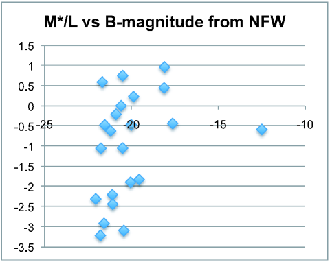
Figure 2: The total-mass-to-light ratios derived from the best fit values and the measured B-band luminosity of the 22 galaxies in dark matter model.

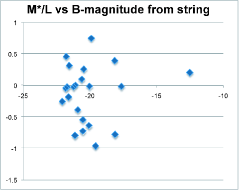
Figure 3: The visible-mass-to-light ratios derived from the best fit values and the measured B-band luminosity of the 22 galaxies in the string model.

2.5.2 The Tully-Fisher Relation

A Tully-Fisher relation can be derived from the string model which relates the rotation velocity in the “flat” region of the rotation curves to the product of the total luminous mass, $M_{stellar}$, and the parameter, $\Omega\,$,

$$v^{3}=GM_{stellar}\Omega~{}.$$ (11)

From the equation of motion (4) we solve for $v$,

$$v=\Omega\,r\,+\,\sqrt{\Omega^{2}\,r^{2}\,+F_{stellar}\,r}~{}.$$ (12)

We then look for a balance of falling Newtonian attraction and rising Lorentz force, resulting in $\frac{\partial v}{\partial r}\sim 0$. Because we know that the turning point is at $r\sim 2.2r_{d}$, setting $\frac{\partial v}{\partial r}\sim 0$ yields a relation between $r_{d}$ and $\Omega$:

$$8\,\Omega^{2}\,\sim\frac{GM_{stellar}}{r^{3}}~{}.$$ (13)

Inside the orbit $r\sim 2.2R_{d}$ lies most of the visible mass. We can therefore use the point-mass approximation when computing $F_{stellar}$ and $\frac{\partial F_{stellar}}{\partial r}$. Upon substituting (13) into (12) our Tully-Fisher relation follows. The string model therefore provides a dynamic origin of this well-tested rule of thumb.

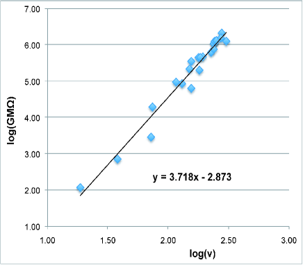
Figure 4: The luminous mass and velocity relation of the 22 galaxies fit by the Tully-Fisher relation derived from the string model.

We plot our best-fit values of $G\,M_{stellar}\,\Omega$ against $v$ in Fig. 4. The representative velocity, $v$, is selected to be the maximal observed velocity in the entire curve for each galaxy, to eliminate man-made bias. This no doubt introduces more scatter than necessary. Despite that the data obey the relation remarkably well.

Note that this is a nontrivial relation because it relates two parameters from two additive force terms to an observed quantity, the rotational speed. Furthermore if one can determine the luminous mass of the galaxy, $M_{stellar}$ and the field strength, $H$, we can determine the fundamental charge-to-mass ratio. This ratio is universal for all matter according to string theory, and is determined by measuring the rotating speed of a test star. Furthermore, our model provides a dynamical explanation to the Tully–Fisher relation.

2.5.3 A Relation Obtained from the String Model Fitting Result

By dimensional analysis, together with some common results from astronomy, we can find a simple relationship between the field strength $\Omega$, galaxy luminosity and size. This serves as a consistency check for the string model. According to the string model, considering its analogy with electromagnetism, it is reasonable to expect the average field strength to be proportional to $M^{\alpha}R^{-\beta}$, where $M$ is the total luminous matter in the galaxy and $R$ is the size scale of the galaxy.  To be more specific we will heavily use the electromagnetism analogy in the following discussion. Consider a group of electrons azimuthal symmetrically distributed and in rotation around the $z$ axis. Let us look at the magnetic field at the center of this distribution, the determining physical quantities are: the magnetic constant $\mu_{0}$, mass density scale $\rho_{0}$, distribution size scale $R_{0}$ and rotational angular velocity scale $\omega_{0}$. 

(Other determining factors include the shape and the spatial dependence of the mass distribution; and the spatial distribution of the angular velocity. These factors do not change the result of dimensional analysis but they do change the proportional constant.) By dimensional analysis, we have

$$B\propto\mu_{0}\cdot\rho_{0}\cdot\omega_{0}\cdot R_{0}^{2}$$ (14)

Using the total charge $Q\propto\rho_{0}\cdot R_{0}^{3}$, and defining $v_{0}=\omega_{0}\cdot R_{0}$, we have

$$B\propto\mu_{0}\cdot Q\cdot R_{0}^{-2}\cdot v_{0}$$ (15)

Note that $v_{0}$ is the rotational velocity scale for the galaxy. Translating to the language of the string model, it is

$$\Omega\propto Q\cdot R_{0}^{-2}\cdot v_{0}$$ (16)

The proportional constant here depends only on the mass and angular velocity distributions, or abstractly on the galaxy type.  Thus galaxies with similar mass distribution profile and rotation curve shapes should have similar constants of proportionality. Now recall $M\propto Q$, where the proportional constant is universal and thus the same for all galaxies. Furthermore we also use the assumption $L~{}\propto~{}M$.  Thus

$$\Omega\propto L\cdot R_{0}^{-2}\cdot v_{0}$$ (17)

To relate $v_{0}$ to $L$ we use the Tully-Fisher relation which says $L~{}\propto~{}\Delta~{}V^{\alpha}$ where $\alpha$ is around $2.5\pm 0.3$ and $\Delta V$ is the velocity width of the galaxy(Tully & Fisher, 1977). The proportional constant in the Tully-Fisher relation is galaxy type independent. Since $v_{0}$ is the overall scale for $\Delta V$, we also have $L~{}\propto~{}(v_{0})^{\alpha}$. Using this in (17), we get

$$\Omega\cdot R_{0}^{2}\propto L^{1+\frac{1}{\alpha}}$$ (18)

which after taking logarithm

$$\ln\left(\Omega R_{0}^{2}\right)=\left(1+\frac{1}{\alpha}\right)\ln\left(L\right)+\ln\kappa$$ (19)

where $\kappa$ is the proportional constant in the relation (18). The log-log diagram is shown in Fig.5.

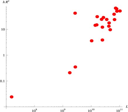
Figure 5: luminosity to $\Omega R^{2}$ log-log plot

There seems to be a trend of a linear relation in the “main” part of the diagram. The slope of the line is about $\frac{3}{2}$, quite close to the $1+\frac{1}{2.5\pm 0.3}$, which was derived theoretically. Two points seems to lie outside of the “main” part, i.e one at the lower left corner for the dwarf galaxy m81dwb, and another one for NGC4236 at the left of the upper right group. In terms of galaxy type these two galaxies are “exotic” among the 22, and thus perhaps their $\ln\kappa$ deviated more from those in the “main” part. Actually in terms of morphology type, NGC4236 is SBdm, which is the most irregular among the regular types, while m81dwb is the only dwarf galaxy among the 22 galaxies from the NED data base (NED, ; Mazzarella et al., 2001). All others are more or less regular galaxies. Presumably these two lie on another line for irregular galaxies which is parallel to the line passing the rest. It is possible that there are a series of parallel lines for different types of galaxies. However, statistical error from the small size of this data set makes the above arguments weak. Using analysis of this kind for a larger number and for more types of galaxies could make the situation clearer; but this exercise is beyond the scope of the current project.

2.6 Discussion

The original appeal of the NFW profile based on the ideas of hierarchical clustering was its universality. One simple NFW profile was expected to explain structure formation, rotation curves of galaxies–giant or dwarf–from high to low surface brightness. This promise has been undermined by the cusp and core debate in dwarf galaxies as well as in the low surface brightness galaxies (see for example (van den Bosch & Swaters, 2001)). The fact that light does not follow dark matter–well established by detailed observation and analysis in the Milky Way (see (Gilmore, 1997) for a summary), in addition to a clear deficit of satellite galaxies in MW have only served to thicken the plot. This debate has recently been taken to a broader context by observational progress: The simplicity of the galaxies (Disney et al., 2008) and the early assembly of the most massive galaxies (Collins et al., 2009) are at odd with the hierarchical clustering paradigm.

While we are not claiming that our string toy model can answer all these questions in one stroke we merely show that it pans out just as well as the Dark Matter model in fitting the galaxy rotation curves while using two fewer parameters. Moreover by tuning the ratio of the strength of the string field to stellar mass density galaxies with a wide range of surface brightness and sizes can be accommodated. We have one dwarf and several LSB galaxies in our sample. At the same time the model, based as it is on a tractable physical principle consistent with laws of mechanics and special relativity, does not suffer from the arbitrariness and puzzling inconsistencies of MOND.

In order to describe a universal galaxy rotation curve (Rubin et al., 1985; Persic et al., 1996; Salucci et al., 2011) one needs three parameters at most–to specify the initial slope, where it bends, and the final slope. Any more parameter are redundant. In this regard the string model utilizes just the right number. The fact that it fits well on par with the dark matter model which employs two extra parameters should be taken seriously. However one should guard against reading too much into the game of fitting. For example, one cannot obtain a unique decomposition of the mass components of a galaxy using the rotation curve data alone, a difficulty encountered in the context of comparing different dark matter halo profiles. Acceptable fits (defined as $\chi<\chi_{min}+1$ (Navarro, 1998)) can be obtained with dark matter alone without any stellar matter in the CDM model. The roles of dark matter and stellar matter can also be completely reverted in the fitting routine. On the other hand, the physical difference is dramatic. This degeneracy is less severe in the string model in the sense that the string field cannot be completely traded off in favour of stellar matter, or vice versa. However a range of values for $R_{d},\rho_{0}$ and $H$, where “acceptable” fits can be obtained, still exists. Therefore given the quality of the available data rotation curve fitting alone cannot distinguish between dark matter and the string field in galaxies.

However precision measurements extended to radii $r\sim 20R_{d}$ can distinguish the string model from the other models: a gently rising rotation curve in this region is a signature prediction of this string toy model. At this moment we are, nevertheless, encouraged by this inchoate results to pursue further. In a separate article we shall subject our string model to other reality checks, and we shall report on how this simple string model accounts for gravitational lensing which is often cited as strong evidence for the existence of dark matter at intergalactic scales.

At this point it is worth mentioning that a critical reanalysis of available data performed by Kuijken and Gilmore on velocity dispersion of F-dwarfs and K-giants in the solar neighborhood, with more plausible models concluded that the data provided no robust evidence for the existence of any missing mass associated with the galactic disk in the neighborhood of the Sun (Kuijken & Gilmore, 1989). Instead a local volume density of $\rho_{0}=0.10M_{sun}pc^{-3}$ is favored, which agrees with the value obtained by star counting. Dark matter would have to exist outside the galactic disk in the form of a gigantic halo. Their pioneer work was later corroborated by (Flynn & Fuchs, 1994; Creze et al., 1998; Pham, 1997; Holmberg & Flynn, 2000; Khriplovich & Pitjeva, 2006a) using other sets of A-star, F-star and G-giant data. Note that this observation can be nicely explained by our model as the field only affects the centripetal motion on the galactic plane; it has no affect on the motion perpendicular to the galactic plane.

We presented a simple string toy model with only one free parameter and we showed that it can fit the galaxy rotation curves equally as well as the dark matter model with the generalized NFW profile. The latter employs two more free parameters compared with the string model. The string model respects all known principles of physics and can be derived from the first principle using string theory, which in turn unifies gravity with other interactions. Our model has an unambiguous prediction concerning the rotation dynamics of satellites and stars far away from the center of the (host) galaxy. The ability to test the validity of string theory as a description of low energy physics makes the exercise worthwhile.

3 Perihelion precession

In this section we test the string model with planetary precession data in the solar system. In (Pitjeva, 2009; Iorio, 2009a), after taking careful account of the influence of all other planets on the orbit of the planet concerned, anomalous precessions for Saturn were reported, for which no explanation within the standard paradigm seems to exist. This anomaly disappeared in successive analyses (Fienga et a. 2011, Pitjev & Pitjeva 2013) in the sense that, nowadays, non-zero extra-precessions at a statistically significant level are absent; however intervals statistically compatible with zero for allowed values for any anomalous precessions are, indeed, obtained. It is thus an interesting laboratory to constrain our string model and ask if the string gauge field can explain the reported ranges of possible anomalous precession. Furthermore, this serves as an independent estimate of the upper bound on the strength of the string field in our galaxy. This estimate can thus be compared to the field strength estimate from the Milky Way rotation curves. It is because we can use the reported ranges of anomalous precession to determine the profile as well as a bound on the strength of the string gauge field inside the solar system. As it turns out, the extra field needed to generate the extra centripetal force to account for the anomalous precession has a profile of a dipole field generated by the Sun. It is then important to compare the magnitudes of field strength as obtained by different methods and observations. A consistent model should give similar values in the field strength for the same object.

3.1 Field Strength from Precession in the Solar System

Here we will use the anomalous precession data to determine the string field profile and field strength in the solar system. We attribute all the anomalous precession to the magnetic like force due to the string field. We are interested in the quantity (Cheung et al., 2007)

$$\Omega=\frac{QH}{m}$$ (20)

where $\frac{Q}{m}$ and $H$ are the string charge-to-mass ratio and the field strength, respectively.  $\Omega$ has the dimension, $s^{-1}$, that of frequency. In other words we are testing the validity of Newtonian gravity in the extremely low frequency regime. The corresponding quantity in electromagnetism is $\frac{eB}{m}$. In these units it is easy for us to compare it with the strengths of other magnetic-like forces, e.g $\frac{eB}{m}$, in electromagnetism. Precession from a magnetic-like force perturbation has been worked out in detail from the first principle in (Xu, 2011) (see also (Ni, 2012; Adkins & McDonnell, 2007; Chashchina & Silagadze, 2008; Ruggiero, 2010; D’Eliseo, 2012; Iorio et al., 2011).)

$$\delta\dot{\omega}=-\left(\frac{qB}{m}\right)\frac{1}{\sqrt{GM_{\odot}}}\pi\left(\frac{a^{\frac{3}{2}}}{T}\right).$$ (21)

To calculate the strength of $\Omega$ using precession data we replace $\frac{qB}{m}$ with $\Omega=\frac{QH}{m}$ in the above formula (21) and invert it to get

$$\Omega=(-\delta\dot{\omega})\sqrt{GM_{\odot}}\frac{T}{\pi a^{\frac{3}{2}}}.$$ (22)

For error analysis, we have

$$\left|\frac{Err(\Omega)}{\Omega}\right|=\left|\frac{Err(\delta\dot{\omega})}{\delta\dot{\omega}}\right|+\frac{1}{2}\left|\frac{Err(GM_{\odot})}{GM_{\odot}}\right|+\frac{3}{2}\left|\frac{Err(a)}{a}\right|.$$ (23)

However, relative errors from other sources are extremely small compared to $\frac{Err(\dot{\delta\omega)}}{\dot{\delta\omega}}$. Indeed, as can be seen from data in table 1, $\frac{Err(\dot{\delta\omega)}}{\dot{\delta\omega}}$ is around order 1, $\frac{Err(a)}{a}\ll 1$. Moreover, $GM_{\odot}=132712440042\pm 10km^{3}/s^{2}$ ((Konopliv et al., 2011) page 425), i.e $\frac{Err(GM_{\odot})}{GM_{\odot}}\sim 10^{-10}$. So we can compute the error by

$$\left|\frac{Err(\Omega)}{\Omega}\right|=\left|\frac{Err(\delta\dot{\omega})}{\delta\dot{\omega}}\right|~{}.$$ (24)

The upper bounds of $\Omega$ determined from precession data are also shown in Table 1, and the fitting results are shown in Fig. 6. $a$, $T$ and $e$ are from HORIZON (HOR, ). Uncertainties in $a$ are from (Pitjeva, 2007) (Table 3).

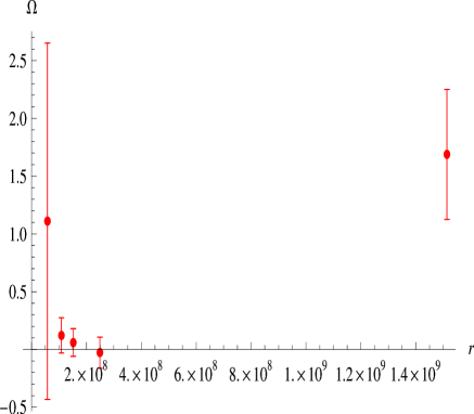
Figure 6: $\Omega(1\times 10^{-17}s^{-1})$ versus distance $r(km)$ to the Sun

The central values of the allowed ranges of $\Omega$ for the inner planets exhibit a decreasing pattern with respect to $r$, although big error bars also allow for the case of the vanishing string field.  At Saturn, $\Omega$ is nonzero within one $\sigma$. However, as mentioned in (Pitjeva, 2009; Iorio, 2009a), the error bar at Saturn may actually be bigger than quoted, in which case the value of precession, or $\Omega$, may vanish. More precise measurements on precession are needed to definitely determine the existence of $\Omega$ (in other words, the anomalous precession rate) in the solar system. Inspired by this decreasing pattern in Appendix A we will fit data of inner planets with a (nearly) power law profile. No matter how critically we take the profile and magnitude of $\Omega$ here, it is–nevertheless–certain that the upper limit of $\Omega$ as deduced from the currently observed ranges of potential anomalous precession of planets in the solar system is on the order of $10^{-17}s^{-1}$, but it can be zero as well.

Planet	$\delta\dot{\omega}$ (I09)	$\Omega$	$\delta\dot{\omega}$ (INPOP08)	$\Omega$	$\delta\dot{\omega}$ (INPOP10a)	$\Omega$
Mercury	$-36\pm 50$	$1.11$	$-100\pm 300$	$3.07$	$4\pm 6$	$-0.123$
Venus	$-4\pm 5$	$1.22\times 10^{-1}$	$-40\pm 60$	$1.22$	$2\pm 15$	$-0.0608$
Earth	$-2\pm 4$	$5.99\times 10^{-2}$	$0\pm 2$	0	$-2\pm 9$	$0.0599$
Mars	$1\pm 5$	$-2.69\times 10^{-2}$	$4\pm 6$	$-0.108$	$-0.4\pm 1.5$	$0.0108$
Saturn	$-60\pm 20$	1.69	$-100\pm 80$	2.81	$1.5\pm 6.5$	$-0.0422$
Planet	$\delta\dot{\omega}$ (P09)	$\Omega$	$\delta\dot{\omega}$ (P13)	$\Omega$
Mercury	$-40\pm 50$	1.23	$-20\pm 30$	0.61
Venus	$240\pm 330$	$-7.30$	$26\pm 16$	-0.79
Earth	$60\pm 70$	$-1.80$	$1.9\pm 1.9$	-0.057
Mars	$-70\pm 70$	1.88	$-0.2\pm 0.37$	0.0054
Saturn	$-100\pm 150$	2.81	$-3.2\pm 4.7$	0.09

Table 1: Anomalous precession rates ($10^{-4}~{}^{\prime\prime}/cy$) and corresponding upper bounds on $\Omega$ ($10^{-17}s^{-1}$). We do not show the uncertainties of $\Omega$ in the table, but they can be obtained from those of $\delta\dot{\omega}$ by the relation $\left|\frac{Err(\Omega)}{\Omega}\right|=\left|\frac{Err(\delta\dot{\omega})}{\delta\dot{\omega}}\right|$. Precession data I09 is from (Iorio, 2009a). INPOP08 and INPOP10a are from ((Fienga et al., 2011a),table 5). P09 is from ((Pitjeva, 2009), table 8). P13 is from ((Pitjev & Pitjeva, 2013), table 5).

As a comparison, let us note that for the real magnetic field near the Earth, $B\sim 10^{-9}~{}\mathrm{Tesla}$, and with $\frac{e}{m}=1.76\times 10^{11}C/kg$, we have $\Omega_{em}\sim 100s^{-1}$. (See Appendix B for details.) In that sense, the string field strength is, naively, $10^{19}$ times smaller than the strength of the magnetic field near the earth. We may wonder why this “strong” magnetic field has not affected precession of planets, and specifically, we can ask if it is related to the observed anomalous precession of planets. One reason why we do not have to worry about the real magnetic field is that planets are electrically neutral (See (Iorio, 2012a)), but charged under the string gauge field as postulated. The real magnetic field can act on neutral matter only through dipole-dipole interaction, which, as explained in Appendix B, does not contribute to planet precession for several reasons.

There is however another question we may ask about the string model now that we are assuming matter is charged under the string field and being acted on by the corresponding magnetic part for this charge: is there an electrical part of the interaction between stringly charged matter? After all, we seem to be assuming that all matter take the “same” kind of charge. This question lies outside of our current model and calls for more theoretical investigations into the nature of this string charge. As for the model used here, we are considering a magnetic interaction in the form of a Lorentz force .

A few words on Saturn are warranted. One aspect special about Saturn is that it belongs to the gas giant group while all other planets considered here are small, solid, and belong to the inner planet family of the solar system. As in the electromagnetic theory, the content and structures of planets may affect their interactions with the string field, which might explain the somewhat anomalous behavior of Saturn. This speculation could be supported if anomalous precession behaviors of other gas giants similar to Saturn can be measured in the future.  We await new data for Uranus, Neptune, and Pluto (Pitjeva, 2012, 2008; Morrison, 1998) as well as data for Jupiter with increased accuracy from the JUNO (Matousek, 2007; Bolton & Juno Science, 2004)  and JUICE (Dougherty et al., 2012) missions.

We would also like to remark that there are other approaches to addressing of the problems of anomalous precession of the planets in the solar system–which are completely independent of ours and invoke different physics. (See (Pitjeva, 2009; Fienga et al., 2011b; Adelberger et al., 2009; Reynaud & Jaekel, 2008) for an overview on how planetary dynamics can be used as a probe for fundamental physics.) The standard method is to extrapolate galactic dark matter to the solar system to estimate its influence on planetary motion: (Khriplovich & Pitjeva, 2006b; Frere et al., 2008). For example, an array of models (Leiva et al., 2012; Mirza & Dehghani, 2002) use non-commutative geometry (e.g. (Cheung & Krogh, 1998; Seiberg & Witten, 1999)). Another large class of models (Dvali et al., 2003; Lue, 2006; Iorio, 2006a, b; Gabadadze & Iglesias, 2008; Battat et al., 2008; Abdujabbarov & Ahmedov, 2010) makes use of induced gravity (Cheung et al., 2004a) in the brane-world a la DPG (see (Maartens & Koyama, 2010; Gabadadze, 2007) for nice reviews.). Yet another way to explain the precession is based on modified newtonian dynamics, MOND, (Boyarsky & Ruchayskiy, 2011; Afshordi et al., 2009; Schmidt, 2008; Iorio, 2009b; Gabadadze & Iglesias, 2008; Iorio & Ruggiero, 2008; Iorio, 2011c, 2009c). Effects from general relativity, as well as the modification of Einstein’s gravity (see, for example (Sotiriou & Faraoni, 2010; Clifton et al., 2012; Hinterbichler, 2012), reviews on modified gravity), are explored in excruciating detail to explain the anomalous precessions of planets. The volume of literature is also large. A random sample of recent literature includes (Ni, 2012; Damour & Lilley, 2008; Iorio & Saridakis, 2012; Iorio, 2012f; Borka et al., 2012; Lecian & Montani, 2009; Reynaud & Jaekel, 2008)). And various other creative approaches: see, for example, (Iorio, 2012c; Arakida, 2012; Gong & Wang, 2009; Kopeikin, 2012; Iorio, 2012b, 2011b, d, 2011d, 2011a, e).

3.2 Field strength from Milky Way rotation curve

In Section 3.1 we obtained $\Omega$ in the solar system from anomalous precession. The constant background value, found by the profile fitting in Appendix A, mainly comes from other matter in the Milky Way. On the other hand, from the same idea used in (Cheung & Xu, 2008), we can also estimate $\Omega$ at the solar system due into the Milky way’s rotation. Thus a natural check of the string model is to compare these two values of $\Omega$: one from the constant background from precession in the solar system and the other one from the rotation curve of the Milky Way.

Directly using the idea in (Cheung & Xu, 2008), we can make a rough estimate of $\Omega$ in the Milky Way as follows. In the string model, the total force on the galaxy mass is composed of only the gravitational attraction from visible mass in the Milky Way and the magnetic-like force from the string field. By increasing $r$, the gravitational force decreases quickly, and the magnetic like force always increases. At the position of the Sun the rotation curve is well into the flat region (Honma & Sofue, 1997; Sofue et al., 1999; Sofue & Rubin, 2001; Battaner & Florido, 2000). Therefore on the Sun the gravitational force should be negligible with respect to the magnetic-like force from the string field. Then (Cheung et al., 2007)

$$m\frac{v^{2}}{r}\approx QHv$$ (25)

and thus

$$\Omega\approx\frac{v}{r}$$ (26)

For the sun (Honma & Sofue, 1997; Sofue et al., 1999; Sofue & Rubin, 2001; Battaner & Florido, 2000), $v_{\odot}\approx 200km\cdot s^{-1}$ and $r_{\odot}\approx 7.6kpc$. So

$$\Omega_{\odot}\approx 26s^{-1}\cdot\frac{km}{kpc}=8.5\times 10^{-16}s^{-1}$$ (27)

This is the upper limit on $\Omega$ due to the Milky Way at the position of the Sun. Since there is still a portion of distance further out to nearly $20kpc$ where the curve is quite flat (with velocity $\sim 200km\cdot s^{-1}$) (Honma & Sofue, 1997; Sofue et al., 1999; Sofue & Rubin, 2001; Battaner & Florido, 2000), we could have used these distances instead of $7.6kpc$ and the value of $\Omega$ will be reduced by a factor of about three. In any case, it is safe to say the upper limit of $\Omega$ is on the order $10^{-16}s^{-1}$. This is the strength of the field component perpendicular to the galactic plane. To convert it to the solar system, note that the north galactic pole and the north ecliptic pole form an angle of 60.2^∘ (which means the field in the solar system would be reduced by almost half), and the Milky Way rotates clockwise when viewed from the north galactic pole (which means the field is negative in the solar system since the planets rotate counterclockwise if viewed from the same direction). Therefore, from the rotation curve of the Milky Way the upper limit of the effective field strength in the solar system due to matter in the milky way is $-10^{-17}$ to $-10^{-16}s^{-1}$. This magnitude is close to the one found by direct precession calculation without the profile assumption, but it is not the case for the field direction. The precession indicates that the field in the solar system is positive, while the rotation curve of the Milky Way says it is negative. One possible explanation is that at places near the Sun, the field is dominated by the positive field the Sun generates, and the Milky Way provides only the constant background in the solar system. The profile fitting of precession, apart from a dipole like part due to the Sun, indeed gives a negative background ($-0.02\times 10^{-17}s^{-1}$). However the magnitude there is smaller by almost two orders of magnitude.

3.3 Field Strength from the Double Pulsar

Here we discuss if we can get a better constraint on $\Omega$ from the precession data of the double pulsar. The double pulsar PSR J0737–3039 is a binary system of two pulsars(Burgay et al., 2003; Iorio, 2009d; Kramer et al., 2006). It is a highly relativistic system and thus has become a laboratory for tests of general relativity. Due to its relativistic nature, the orbits of the solar system’s members have a huge perihelion (periastron) precession rate $\dot{\omega}=16.89947(68)$deg/yr ((Kramer et al., 2006), Table 1). After subtracting the first order post-Newtonian contribution from precession, the remaining “unexplained” precession rate is ((Iorio, 2009d), Equation (14))

$$\delta\dot{\omega}=\dot{\omega}_{exp}-\dot{\omega}_{1PN}=-0.00463\pm 0.03233~{}\mathrm{deg/yr}.$$ (28)

This value of precession imposes a bound on the magnitude of $\Omega$ at the system’s location. For the system, the orbit period $T=0.10225156248(5)$ day, the projected semi-major axis $a\sin i=1.415176(5)\mathrm{light~{}s}$, for which $i\approx 90^{\circ}$ is the inclination angle, and the total mass is $2.85(2)M_{\odot}$ (Kramer et al., 2006; Iorio, 2009d). Here we only consider the order of magnitude of the constraint on $\Omega$, so we can use these values directly in the Equation (22). The result is

$$\Omega=-10431^{\prime\prime}\pm 72840^{\prime\prime}/\mathrm{cy}=-(1.6\pm 11.2)\times 10^{-11}s^{-1}.$$ (29)

This is a bound on $\Omega$ much higher than those from rotation curves and precessions of planets in the Solar system. Therefore the double pulsar does not give a better constraint on $\Omega$. Also note that the large uncertainty allows for the case $\Omega=0$.

3.4 Discussion

With the latest reported ranges of the possible anomalous precession of planets in the solar system, we obtained upper limits on the field strength of the string gauge field–attributed to universally coupling to all matter–at several places in the solar system. The maximal field strength allowed in the orbit of, say, Mercury is found to be on the order of $10^{-17}s^{-1}$. The distribution of the field in the solar system looks like a superposition of a constant background field and a $r^{-3}$ decreasing “dipole” component in (A1).We discussed a possible configuration where the Milky Way produced the constant background field and the Sun produced the “dipole” component. A profile fitting is done for this configuration, with details provided in Appendix A. The background is found to be negative, which, when combined with analysis using electromagnetism analogy, correctly matches with the fact that the solar system and the Milky Way rotate in opposite directions.

As a comparison with the field strength obtained from precession in the solar system, we estimated the upper limit on the field strength of the string gauge field in the Milky Way directly from the rotation curve of the Milky Way at the position of the Sun. This estimate has an order of magnitude similar to that from precession. However, the direction is opposite. If we consider the background-plus-dipole-field configuration used for profile fitting to be correct, then we should consider only the background value when comparing with the one estimated by the Milky Way rotation curve. In that case, the background direction agrees with the one predicted by the Milky Way rotation curve, but the magnitude is smaller by 2 orders of magnitude.

4 Summary

We discussed the possibility that the rotational speed of the stars at the center of a spiral galaxy is supported by the presence of string gauge field which couples universally to all forms of matter. We compared the goodness of fit of the string model to that of the commonly accepted CDM model with the generalized NFW profile for DM distribution . We fit rotational speed data of 22 spiral galaxies of varied size and luminosity. DM model fits marginally better ($9\%$)at the price of two more free parameters than the string model. A Tully–Fisher relation relating the visible mass and field strength of the string gauge field to velocity $GM_{star}\Omega=v^{3}$ can be derived dynamically from the string model, which is obeyed fairly well by all 22 galaxies of varied sizes and luminosities.

The existence of the string gauge field is taken a step further and is applied to explain the currently reported ranges of potential anomalous precession of planets in the solar system. The extra field needed to generate the extra centripetal force to account for the anomalous precession has a profile of a dipole field generated by the Sun.

The values–or upper bound in the case of planetary precession–of string fields, which are

• galaxy rotation curves of a set of 22 galaxies (without the Milky way),

• potential perihelion precession of some planets in the solar system and

• the Milky Way rotation curve,

are summarized in Table 2.

	Solar System $\subset$	Milky Way	22 other galaxies
Rotation Curve		$|\Omega|\lesssim 10^{-16}$	$6\times 10^{-18}\lesssim|\Omega|\lesssim 10^{-15}$
Precession	$|\Omega|\lesssim 0.61\times 10^{-17}$

Table 2: Dimension for $\Omega$ is $s^{-1}$. Note: the first column indicates the kind of observation used, and the first row indicates the object observed.

Interestingly–and also luckily for the string model–the results from these different methods lead to a similar order of magnitude for $\Omega$.

While supersymmetry is losing some of its lust because of is has not been detected in LHC (Santanastasio, 2013; Golling et al., 2013; Delgado et al., 2012; Chatrchyan et al., 2013b, c; Aad et al., 2012a; Chatrchyan et al., 2012, 2013a; Aad et al., 2012b, 2011), DM is also losing its most celebrated candidate, the lightest supersymmetric neutral particle. (See, for example, (Arkani-Hamed et al., 2012; Ibanez & Valenzuela, 2013; Murayama et al., 2012) for possible explanations of the no show.) The game of explaining the missing matter in the universe is becoming intriguing again.

Appendix A Profile fitting of precession in solar system

The decreasing pattern of $\Omega$ for inner planets with respect to $r$ indicates it might be useful to fit these values with a power law term. Presumably we could attribute this $r$ dependent term to the Sun from which $r$ is measured. On the other hand, note that $\Omega$ at the Mars is negative, although it seems also sitting on the same curve passing the first three inner planets.

One possible configuration for $\Omega$ compatible with these 2 facts is then that, in addition to a power law term, there is also a weak constant background $\Omega$ with opposite direction to the $\Omega$ from the Sun. The constant background might be provided by all other matter in the universe. The Milky Way should be the most important source of this influence. Here we try to fit field strength at different inner planets with the following profile,

$$\Omega(r)=A+Br^{-a}$$ (A1)

For the actual fitting on computer, the profile used is

$$\Omega(r)=\Omega_{0}+\Omega_{1}\left(\frac{r}{10^{7}km}\right)^{-a}$$ (A2)

The best fitting parameters for this profile is

$$\Omega_{0} =-0.0223787\times 10^{-17}s^{-1}$$ (A3)

$$\Omega_{1} =260.504\times 10^{-17}s^{-1}$$

$$a =3.09953$$

It is helpful to know the relative strength of the two components from the Sun and the constant background, which is shown in Table 3.

Planet	Mercury	Venus	Earth	Mars
ratio	50.3	7.1	2.5	0.54

Table 3: relative strength: power law term/constant term

The power law term decreases with $r$ quickly relative to the background. We can safely say that in most areas in the solar system, the string field would just be around that background, which is on the order of $10^{-19}$Hz. And that $a$ is found to be near 3, which is exactly the power for a dipole field. It means that the string field interaction between the sun and planets is similar to that between a magnetic dipole and charged particles.

Also note that the fitting result tells us that the constant background in the solar system is negative. This is good news for the string model. As in electromagnetism, we expect the string gauge field in a galaxy to be generated by the rotation of matter (charged under the string gauge field) in the galaxy, just like rotating electric charge would generate a magnetic field. Since the Sun and planets in the solar system rotate in the opposite direction of that of stars’ rotation in the Milky Way, it is therefore reasonable to expect the background field to be negative if we consider the one from the Sun as positive. This is exactly what the profile fitting has told us. Here only data of the solar system was used, but the conclusion is for the whole Milky Way, specifically for its rotation direction.

However, this conclusion should be taken with a grain of salt, as we will explain below. Firstly, the long error bars of precession weaken the conclusion from this profile fitting. Secondly, there exists possibilities for the field from the Sun to be in the same direction with that of the Milky way. As in ordinary electromagnetic theory, for a right handed current disk the magnetic field is downward outside of the major current distribution, but upward if we go into the current disk somewhere, specifically at the center of the disk. There is a place within the concentration where the magnetic field changes its sign.  Thus even if the Milky Way is rotating in opposite direction from the solar system, if the Sun is too close inside the major mass concentration of the Milky Way, the background should still be positive. To our advantage, it is known that the Sun contains 99% of the total mass in the solar system, so it is reasonable to assume all planets are well outside of most mass in the solar system. And the solar system lies somewhat outside the majority of mass concentration of the Milky Way.

Appendix B Solar system magnetic field and its effect on planet perihelion precession

References for this appendix are Parker (1958); E.N.Parker (1958); Shirley & Fairbridge (1997); Meyer et al. (1956); Babcock (1961). The Sun and most planets in the solar system have magnetic field due to dynamo effect. If we treat both the Sun and the planet as magnetic dipoles interacting in vacuum (which leads to a central force with $n=-4$), using data of magnetic fields of the Sun (around $1\sim 2$ gauss at the polar region) and the Earth (around 0.6 gauss at the polar region), we can find the corresponding precession produced is nearly $10^{-6}$arcsec/cy, which is 2 orders of magnitude smaller than the observed one. In fact the magnetic field in the solar system is much more complicated than those produced by several dipoles in vacuum. First, the solar system is not empty but filled with particles emitted from the Sun, i.e the solar wind. Charged particles lock with it the magnetic field of the Sun and spread it all around in the solar system. From the Sun to about the position of the Earth, the magnetic force line is parallel to the radial stream of solar wind particle and falls off by $r^{-2}$. From the position of the Earth to about position of the Mars is a field free region with $B<10^{-6}$ gauss. Further out to the position of the Jupiter is a region with disordered magnetic field with $B\sim 10^{-5}$ gauss. For precession, the most important feature of the solar system field is that it is oscillating. First, for the Sun the magnetic dipole axis is inclined relative to the rotational axis. This leads to an oscillating neutral current sheet. Therefore planets on the ecliptic plane is above the neutral current sheet for half of solar self rotation period, below for another half. Since field directions above and below the neutral current sheet is opposite, the magnetic force experienced by the planets also change directions within one self rotation of the Sun. Second, the magnetic field of the Sun also changes direction every 22 years due to its differential rotation, which leads to another oscillation of magnetic field on the planets. Altogether these two oscillations make the magnetic field effect on precession neglectable with respect to other accumulating effects.

Appendix C Different fitting models give different best fittings

Fitting a galaxy consists of following steps:

• assume a density profile (a parametric description of the density),

• adjust the values of free parameters to minimize an “error function.”

The corresponding resulting parameters are called best fitting parameters. For a single galaxy we can define different error functions. It can be defined by rotation curve, by surface brightness or some other observation data. The point of this appendix is that we usually get different best fitting parameters when using different error functions. In particular, best fitting parameters for rotation curve are different from those for surface brightness. Below we provide a simple and idealized example to illustrate this point.

Real

Suppose the real density distribution is a linearly decreasing function of radius and becomes zero outside of a cutoff radius,

$$\rho(r)=\Bigl{\{}\begin{array}[]{cc}\rho_{0}(1-\frac{r}{R}),&(0\leq r\leq R)\\ 0.&(r\geq R)\end{array}$$ (C3)

where $\rho_{0}$ and $R$ are two fixed constants for this particular galaxy.  The corresponding velocity, using Newtonian gravitation theory, is

$$v(r)=\Biggl{\{}\begin{array}[]{cc}\sqrt{2\pi\rho_{0}G_{N}(\frac{1}{2}-\frac{1}{3}\frac{r}{R})r},&(0\leq r\leq R),\\ \sqrt{2\pi\rho_{0}G_{N}\frac{1}{6}\frac{R^{2}}{r}},&(r\geq R)\end{array}$$ (C6)

and brightness is (assuming light is proportional to mass) where $\gamma$ is light to mass ratio. Which gravity theory we use does not affect the conclusion of this appendix, so long as we use the same theory for any profile to derive the velocity.

$$B(r)=\Bigl{\{}\begin{array}[]{cc}\gamma\rho_{0}(1-\frac{r}{R}),&(0\leq r\leq R),\\ 0,&(r\geq R)\end{array}$$ (C9)

Guessed

Without knowing the real distribution, suppose we assumed for this galaxy a constant distribution profile

$$\rho(r)=\Bigl{\{}\begin{array}[]{cc}\sigma,&(0\leq r\leq D)\\ 0.&(r\geq D)\end{array}$$ (C12)

Here $\sigma$ and $D$ are two parameters, rather than constants, being fitted to get best fitting values, while $\rho_{0}$ and $R$ have particular fixed values for this galaxy. This density profile produces following velocity profile

$$v(r)=\Biggl{\{}\begin{array}[]{cc}\sqrt{\pi\sigma G_{N}r},&(0\leq r\leq D),\\ \sqrt{\pi\sigma G_{N}D^{2}\frac{1}{r}},&(r\geq D),\end{array}$$ (C15)

and brightness profile

$$B(r)=\Bigl{\{}\begin{array}[]{cc}\gamma\sigma,&(0\leq r\leq D)\\ 0,&(r\geq D).\end{array}$$ (C18)

Fitting

As said before, we can define different error functions to do the fitting. We can use either rotation velocity or brightness for fitting. Ideally the error functions can be defined respectively for rotation velocity and surface brightness by

$$\chi_{v}^{2}(D,\sigma)=\int_{0}^{\infty}dr^{\prime}[v_{model}(r^{\prime},D,\sigma)-v_{real}(r^{\prime})]^{2}$$ (C19)

$$\chi_{B}^{2}(D,\sigma)=\int_{0}^{\infty}dr^{\prime}[B_{model}(r^{\prime},D,\sigma)-B_{real}(r^{\prime})]^{2}$$ (C20)

After minimizing these two error functions we get two sets of best fitting parameters for $D$ and $\sigma$. Let’s denote the best fitting value for velocity error function $\chi_{v}^{2}$ by $(D_{A},\sigma_{A})$, for brightness error function $\chi_{B}^{2}$ by $(D_{B},\sigma_{B})$. Below we show these two sets of values do not coincide.

If we use the error function for brightness, obviously the best fitting parameters are

$$D_{B}=R,~{}\sigma_{B}=\frac{1}{2}\rho_{0}$$ (C21)

To show $(D_{B},\sigma_{B})\neq(D_{A},\sigma_{A})$ it is sufficient to show that $(D_{B},\sigma_{B})$ does not minimize $\chi_{v}^{2}$. For simplicity we take units such that

$$\rho_{0}=1,~{}~{}~{}R=1,~{}~{}~{}\gamma=1,~{}~{}~{}\pi G_{N}=1,$$ (C22)

then

$$D_{B}=1,~{}~{}~{}\sigma_{B}=\frac{1}{2}.$$ (C23)

In this unit system the real velocity is

$$v(r)=\Biggl{\{}\begin{array}[]{cc}\sqrt{\frac{r}{2}},&(0\leq r\leq 1),\\ \sqrt{\frac{1}{2r}},&(r\geq 1).\end{array}$$ (C26)

Taking 100000 as the upper limit of the integration, we find

$$\chi_{v}^{2}(D_{B}=1,\sigma_{B}=0.5)=0.2,$$ (C27)

$$\chi_{v}^{2}(D=0.9,\sigma=0.5)=0.05$$ (C28)

Thus $(D_{B},\sigma_{B})\neq(D_{A},\sigma_{A})$. The best fitting parameters for brightness do not best fit the velocity curve.

Remarks

Above we considered a simple and idealized galaxy and showed that best fitting parameters for different error functions are in general different, although we were doing the fitting for the same galaxy. Another point worth noting here is that if we had guessed at the correct density profile (which linearly decreases and vanishes beyond some cutoff radius), the two best fitting parameters will be the same. We get different fitting results because we used a “wrong” profile for this galaxy. In real life the mass distribution for a galaxy is extremely complicated and can not be exactly described by any simple “profile function.” Hence after we assume the profile, define the error function and then do the fitting, we will always get different fitting results for “independent” error functions (e.g velocity and brightness). If the guessed profile is closer to the real distribution we get closer results for fittings by different error functions. In other words, a big difference between fitting results by different error functions means the profile we guessed at is very different from the real one.

Given different profile assumptions for the galaxy distribution, we thus have a way to judge in some sense which one is more “correct”. With each profile we can derive corresponding distributions of velocity, brightness and so on, and with each of these distributions we can compute( if we have the data) an error function $\chi^{2}$, which is dependent on a set of parameters owned by this profile,

$$\mbox{Density Profile}\longrightarrow\Biggl{\{}\begin{array}[]{cc}\mbox{Velocity}&\chi^{2}_{v}\\ \mbox{Brightness}&\chi^{2}_{B}\\ \vdots&\vdots\end{array}$$ (C31)

If the profile perfectly match the real one, there exists a single set of parameters simultaneously making all $\chi^{2}$ zero. On the other hand, if the profile differs too much from the real one, even if we can make one of the $\chi^{2}$ small, the corresponding parameters will usually make other $\chi^{2}$’s very large. Therefore it makes sense to use, e.g. the average of several $\chi^{2}$’s as the error function to be minimized. This profile, with the corresponding minimizing parameters of the average error function, best describes the distribution averagely, i.e. considering distributions whose $\chi^{2}$ is averaged.

However we cannot use this to find the real distribution. We can only compare profiles given their profile assumptions and say which is better in describing velocity, brightness and so on, or if we use some averaged error function, also say which is better considering their general performances in describing various properties simultaneously.

Appendix D Detailed Fitting Results of 22 galaxies using dark matter model and using string model

In this appendix we present all the results on the data fitting. Table 4 summarizes the relevant data for luminosity as well as for distance determination. In Table 5 and Table 6 the best fit values for the five free parameters in the dark matter fitting and three free parameter in the string model fitting are presented. Mass of the stellar mass and dark matter halos (in the case of dark matter model) as well as the mass to light ratios are computed from the best fit values for each galaxy. These values are tabulated in Table 7 (dark matter) and in Table 8 (string). The rest of the appendix presents 22 graphs of dark matter fit and string fit side by side for each of the 22 galaxies. In each of the graph small cubes with error bars represent observational data the other symbols, and the curves, represent theoretical values. The X-axis is radius in $kpc$ and Y-axis is velocity in $kms^{-1}$.

galaxy	B-magnitude	mucin	Distance(Mpc)
m81dwb	-12.5	N/A	3.5
ngc0628	-20.60	29.95	9.77
ngc0925	-20.05	29.85	9.33
ngc2403	-19.56	27.68	3.44
ngc2976	-18.12	28.10	4.17
ngc3031	-21.54	28.57	5.18
ngc3184	-19.88	30.20	10.96
ngc3198	-20.44	30.42	12.13
ngc3521	-21.08	30.29	11.43
ngc3621	-20.51	29.58	8.24
ngc3938	-20.01	30.81	14.52
ngc4236	-18.10	27.08	2.61
ngc4321	-22.06	31.90	23.99
ngc4536	-21.79	32.11	26.42
ngc4569	-21.10	30.52	12.71
ngc4579	-21.68	31.80	22.91
ngc4625	-17.63	30.35	11.75
ngc4725	-21.76	31.45	19.50
ngc5055	-21.20	30.09	10.42
ngc5194	-20.51	30.01	10.05
ngc6946	-20.89	29.12	6.67
ngc7331	-21.58	30.75	14.13

Table 4: Relevant galaxy observation data for determining luminosity and distance.

galaxy	likelihood	$R_{d}(kpc)$	$\frac{r_{s}}{R_{d}}$	$\alpha$	$\rho$	$\sigma$
m81dwb	0.158	0.24	8.2	1.54	613	19.2
ngc0628	4.398	1.88	9.9	0.75	8409	98.4
ngc0925	2.392	0.79	27.6	0.22	859	56.6
ngc2403	4.467	0.75	21.1	0.76	744	84.6
ngc2976	0.504	2.52	18.3	0.38	998	16.8
ngc3031	5.614	3.99	5.9	0.96	705	57.7
ngc3184	0.573	3.97	6.1	0.58	784	42.1
ngc3198	0.441	0.51	18.2	1.09	291	99.95
ngc3521	0.167	0.57	18.8	1.56	1738	99.5
ngc3621	0.125	6.85	1.8	1.80	903	5.6
ngc3938	0.905	2.45	5.5	1.33	747	60.6
ngc4236	1.180	4.40	6.5	0.83	603	1.4
ngc4321	0.956	0.87	19.6	1.02	1581	80.5
ngc4536	0.598	0.99	10.7	0.86	105	97.2
ngc4569	0.651	0.74	18.1	0.95	1350	145.4
ngc4579	0.719	7.90	4.3	1.80	1200	3.4
ngc4625	0.874	1.91	14.1	0.20	191	42.6
ngc4725	0.481	4.00	7.5	0.77	225	53.9
ngc5055	1.133	2.25	4.5	1.66	2044	67.0
ngc5194	0.442	1.45	4.4	1.50	1518	49.9
ngc6946	5.670	2.62	29.4	0.27	2491	42.6
ngc7331	0.839	0.50	19.6	1.32	1325	197.7

Table 5: Best fit values for the five free parameters in the Dark Matter model with generalized NFW profile.

galaxy	likelihood	$\Omega$(Hz$\cdot$km$/$kpc)	$\rho$	$R_{d}$(kpc)
m81dwb	0.125	1.119	15919	0.15
ngc0628	4.347	8.872	11738	1.80
ngc0925	2.452	5.077	500	2.47
ngc2403	4.247	13.418	16497	0.52
ngc2976	0.400	0.100	2135	1.87
ngc3031	5.698	2.000	3187	4.39
ngc3184	0.574	0.655	1552	4.69
ngc3198	0.275	1.968	1971	3.52
ngc3521	0.588	6.046	26678	1.48
ngc3621	0.366	10.338	7413	1.08
ngc3938	1.030	9.722	16199	1.24
ngc4236	0.325	10.358	110	2.02
ngc4321	2.070	5.208	3752	3.15
ngc4536	0.739	1.465	734	5.87
ngc4569	0.662	16.370	12262	1.04
ngc4579	0.688	7.385	5164	3.00
ngc4625	0.548	0.100	1140	1.45
ngc4725	0.268	1.378	1523	6.73
ngc5055	3.521	4.064	24581	1.54
ngc5194	0.807	3.186	10718	1.10
ngc6946	6.035	7.440	4980	1.80
ngc7331	0.522	8.465	18613	1.68

Table 6: Best fit values for the three free parameters in the string model.

galaxy	B-magnitude	M∗	DM+M*	M/L	log(M/L)	M*/DM
m81dwb	-12.5	4.07E+06	7.89E+08	50.72	1.71	3.12%
ngc0628	-20.60	2.74E+10	3.34E+12	123.36	2.09	1.00%
ngc0925	-20.05	2.08E+08	2.26E+12	138.71	2.14	0.16%
ngc2403	-19.56	1.55E+08	1.70E+12	164.12	2.22	0.07%
ngc2976	-18.12	7.79E+09	4.79E+12	1738.70	3.24	0.14%
ngc3031	-21.54	2.17E+10	3.83E+12	59.63	1.78	3.42%
ngc3184	-19.88	2.39E+10	2.46E+12	176.74	2.25	3.16%
ngc3198	-20.44	1.88E+07	4.71E+11	20.18	1.30	8.90%
ngc3521	-21.08	1.54E+08	8.70E+11	20.68	1.32	4.83%
ngc3621	-20.51	1.41E+11	1.94E+11	7.81	0.89	2.37%
ngc3938	-20.01	5.35E+09	8.86E+11	56.45	1.75	1.70%
ngc4236	-18.10	2.51E+10	7.30E+10	27.01	1.43	0.61%
ngc4321	-22.06	5.11E+08	2.20E+12	21.25	1.33	2.58%
ngc4536	-21.79	4.96E+07	6.24E+11	7.71	0.89	11.57%
ngc4569	-21.10	2.67E+08	2.09E+12	48.82	1.69	0.32%
ngc4579	-21.68	2.88E+11	8.96E+11	12.26	1.09	7.57%
ngc4625	-17.63	6.45E+08	2.95E+12	1683.06	3.23	0.06%
ngc4725	-21.76	7.00E+09	6.76E+12	85.89	1.93	3.34%
ngc5055	-21.20	1.13E+10	5.00E+11	10.64	1.03	8.81%
ngc5194	-20.51	2.25E+09	8.27E+10	3.32	0.52	8.44%
ngc6946	-20.89	2.19E+10	7.09E+13	2006.87	3.30	0.02%
ngc7331	-21.58	8.09E+07	1.33E+12	19.92	1.30	3.24%

Table 7: Summary of stellar mass and mass of dark matter halos computed from the best fit values, as well as mass to light ratios of the 22 galaxies in the dark matter model. The mass is in units of $M_{sun}$. Mass to light ratio is relative to the mass of light ratio of the Sun.

galaxy	B-magnitude	$\Omega$(Hz$\cdot$km/kpc)	total mass($M_{sun}$)	mass/light
m81dwb	-12.5	1.1193	2.46E+07	1.5814
ngc0628	-20.60	8.8716	3.35E+10	1.2388
ngc0925	-20.05	5.08	3.68E+09	0.2261
ngc2403	-19.56	13.4183	1.12E+09	0.1076
ngc2976	-18.12	0.10	6.76E+09	2.4549
ngc3031	-21.54	2.00	1.31E+11	2.0420
ngc3184	-19.88	0.6553	7.77E+10	5.5805
ngc3198	-20.44	1.9685	4.19E+10	1.7963
ngc3521	-21.08	6.0462	4.20E+10	0.9990
ngc3621	-20.51	10.3377	4.60E+09	0.1848
ngc3938	-20.01	9.7216	1.50E+10	0.9577
ngc4236	-18.10	10.3577	4.42E+08	0.1636
ngc4321	-22.06	5.2077	5.70E+10	0.5492
ngc4536	-21.79	1.4650	7.22E+10	0.8919
ngc4569	-21.10	16.37	6.75E+09	0.1575
ngc4579	-21.68	7.39	6.79E+10	0.9286
ngc4625	-17.63	0.10	1.68E+09	0.9565
ngc4725	-21.76	1.3785	2.26E+11	2.8680
ngc5055	-21.20	4.0642	4.40E+10	0.9373
ngc5194	-20.51	3.1862	6.98E+09	0.2803
ngc6946	-20.89	7.4403	1.43E+10	0.4037
ngc7331	-21.58	8.4646	4.30E+10	0.6446

Table 8: Summary of stellar mass as well as mass to light ratios as computed from the best fit values in string model. The mass of the galaxies is in units of $M_{sun}$. Mass to light ratio is relative to the mass of light ratio of the Sun.

Figure 7: Rotation curve of dwarf galaxy m81dwb fit with the dark matter model (left) and with the string model (right). The $\chi$-squared value per degree of freedom using the dark matter model with a NFW profile is $0.158$ while that using the string model is $0.1254$.

Figure 8: Rotation curve of NGC 0628 fit with the dark matter model (left) and with the string model (right). The $\chi$-squared value per degree of freedom using the dark matter model with a NFW profile is $4.398$ while that using the string model is $4.3468$.

Figure 9: Rotation curve of ngc 0925 fit with the dark matter model (left) and with the string model (right). The $\chi$-squared value per degree of freedom using the dark matter model with a NFW profile is $2.392$ while that using the string model is $2.4518$.

Figure 10: Rotation curve of NGC2403 fit with the dark matter model (left) and with the string model (right). The $\chi$-squared value per degree of freedom using the dark matter model with a NFW profile is $4.467$ while that using the string model is $4.2468$.

Figure 11: Rotation curve of ngc 2976 fit with the dark matter model (left) and with the string model (right). The $\chi$-squared value per degree of freedom using the dark matter model with a NFW profile is $0.504$ while that using the string model is $0.4001$.

Figure 12: Rotation curve of ngc 3031 fit with the dark matter model (left) and with the string model (right). The $\chi$-squared value per degree of freedom using the dark matter model with a NFW profile is $5.614$ while that using the string model is $5.6977$.

Figure 13: Rotation curve of NGC 3184 fit with the dark matter model (left) and with the string model (right). The $\chi$-squared value per degree of freedom using the dark matter model with a NFW profile is $0.573$ while that using the string model is $0.5740$.

Figure 14: Rotation curve of ngc 3198 fit with the dark matter model (left) and with the string model (right). The $\chi$-squared value per degree of freedom using the dark matter model with a NFW profile is $0.441$ while that using the string model is $0.2748$.

Figure 15: Rotation curve of ngc 3521 fit with the dark matter model (left) and with the string model (right). The $\chi$-squared value per degree of freedom using the dark matter model with a NFW profile is $0.167$ while that using the string model is $0.5875$.

Figure 16: Rotation curve of NGC3621 fit with the dark matter model (left) and with the string model (right). The $\chi$-squared value per degree of freedom using the dark matter model with a NFW profile is $0.125$ while that using the string model is $0.3658$.

Figure 17: Rotation curve of ngc 3938 fit with the dark matter model (left) and with the string model (right). The $\chi$-squared value per degree of freedom using the dark matter model with a NFW profile is $0.905$ while that using the string model is $1.0304$.

Figure 18: Rotation curve of ngc 4236 fit with the dark matter model (left) and with the string model (right). The $\chi$-squared value per degree of freedom using the dark matter model with a NFW profile is $1.180$ while that using the string model is $0.3255$.

Figure 19: Rotation curve of NGC4321 fit with the dark matter model (left) and with the string model (right). The $\chi$-squared value per degree of freedom using the dark matter model with a NFW profile is $0.956$ while that using the string model is $2.0703$.

Figure 20: Rotation curve of NGC4536 fit with the dark matter model (left) and with the string model (right). The $\chi$-squared value per degree of freedom using the dark matter model with a NFW profile is $0.598$ while that using the string model is $0.7394$.

Figure 21: Rotation curve of ngc 4569 fit with the dark matter model (left) and with the string model (right). The $\chi$-squared value per degree of freedom using the dark matter model with a NFW profile is$0.651$ while that using the string model is $0.6621$.

Figure 22: Rotation curve of NGC 4579 fit with the dark matter model (left) and with the string model (right). The $\chi$-squared value per degree of freedom using the dark matter model with a NFW profile is $0.719$ while that using the string model is $0.688$.

Figure 23: Rotation curve of ngc 4625 fit with the dark matter model (left) and with the string model (right). The $\chi$-squared value per degree of freedom using the dark matter model with a NFW profile is $0.874$ while that using the string model is $0.5478$.

Figure 24: Rotation curve of ngc 4725 fit with the dark matter model (left) and with the string model (right). The $\chi$-squared value per degree of freedom using the dark matter model with a NFW profile is $0.481$ while that using the string model is $0.2683$.

Figure 25: Rotation curve of NGC 5055 fit with the dark matter model (left) and with the string model (right). The $\chi$-squared value per degree of freedom using the dark matter model with a NFW profile is $1.133$ while that using the string model is $3.5208$.

Figure 26: Rotation curve of ngc 5194 fit with the dark matter model (left) and with the string model (right). The $\chi$-squared value per degree of freedom using the dark matter model with a NFW profile is $0.442$ while that using the string model is $0.8067$.

Figure 27: Rotation curve of ngc 6946 fit with the dark matter model (left) and with the string model (right). The $\chi$-squared value per degree of freedom using the dark matter model with a NFW profile is $5.670$ while that using the string model is $6.0346$.

Figure 28: Rotation curve of NGC 7331 fit with the dark matter model (left) and with the string model (right). The $\chi$-squared value per degree of freedom using the dark matter model with a NFW profile is $0.839$ while that using the string model is $0.5221$.

References

- Aad et al. (2011) Aad, G., et al. 2011, Phys.Rev.Lett., 106, 131802
- Aad et al. (2012a) —. 2012a, Eur.Phys.J., C72, 2215
- Aad et al. (2012b) —. 2012b, Phys.Rev., D85, 012006
- Abdujabbarov & Ahmedov (2010) Abdujabbarov, A., & Ahmedov, B. 2010, Physical Review D, 81, 044022
- Adelberger et al. (2009) Adelberger, E. G., Battat, J., Currie, D., et al. 2010, The Astronomy and Astrophysics Decadal Survey, Science White Papers, no. 300, arXiv:0902.3004
- Adkins & McDonnell (2007) Adkins, G. S., & McDonnell, J. 2007, Physical Review D, 75, 082001
- Adriani et al. (2009) Adriani, O., et al. 2009, Nature, 458, 607
- Afshordi et al. (2009) Afshordi, N., Geshnizjani, G., & Khoury, J. 2009, JCAP, 0908, 030
- Anderson et al. (2004) Anderson, J. D., Lau, E. L., Schubert, G., & Palguta, J. L. 2004, Gravity inversion considerations for radio Doppler data from the JUNO Jupiter polar orbiter. In Bulletin of the American Astronomical Society (Vol. 36, p. 1094).
- Arakida (2012) Arakida, H. 2012, International Journal of Theoretical Physics, at press, doi:10.1007/s10773-012-1458-2, arXiv:1212.6289
- Arkani-Hamed et al. (2012) Arkani-Hamed, N., Gupta, A., Kaplan, D. E., Weiner, N., & Zorawski, T. 2012, arXiv:1212.6971
- Avalos-Vargas & Ares de Parga (2011) Avalos-Vargas, A., & Ares de Parga, G. 2011, The European Physical Journal Plus, 126, 1
- Babcock (1961) Babcock, H. W. 1961, Astrophysical Journal, 133
- Battaner & Florido (2000) Battaner, E., & Florido, E. 2000, Fund.Cosmic Phys., 21, 1
- Battat et al. (2008) Battat, J. B., Stubbs, C. W., & Chandler, J. F. 2008, Phys.Rev., D78, 022003
- Bolton & Juno Science (2004) Bolton, S. J., & Juno Science. 2004, in Bulletin of the American Astronomical Society, Vol. 36, AAS/Division for Planetary Sciences Meeting Abstracts #36, 1092
- Borka et al. (2012) Borka, D., Jovanovic, P., Jovanovic, V. B., & Zakharov, A. 2012, Phys.Rev., D85, 124004
- Boyarsky & Ruchayskiy (2011) Boyarsky, A., & Ruchayskiy, O. 2011, Phys.Lett., B695, 365
- Burgay et al. (2003) Burgay, M., D’Amico, N., Possenti, A., et al. 2003, Nature, 426, 531
- Chang et al. (2008) Chang, J., et al. 2008, Nature, 456, 362
- Chashchina & Silagadze (2008) Chashchina, O., & Silagadze, Z. 2008, Phys.Rev.D77:107502, 2008, arXiv:0802.2431
- Chatrchyan et al. (2012) Chatrchyan, S., et al. 2012, Phys.Rev.Lett., 109, 071803
- Chatrchyan et al. (2013a) —. 2013a, JHEP, 1302, 036
- Chatrchyan et al. (2013b) —. 2013b, arXiv:1301.3792
- Chatrchyan et al. (2013c) —. 2013c, JHEP, 1301, 077
- Cheung & Krogh (1998) Cheung, Y., & Krogh, M. 1998, Nuclear Physics B, 528, 185
- Cheung et al. (2004a) Cheung, Y., Laidlaw, M., & Savvidy, K. 2004a, Journal of High Energy Physics, 2004, 028
- Cheung et al. (2004b) Cheung, Y.-K. E., Freidel, L., & Savvidy, K. 2004b, JHEP, 02, 054
- Cheung et al. (2007) Cheung, Y.-K. E., Savvidy, K., & Kao, H.-C. 2007, arXiv:astro-ph/0702290
- Cheung & Xu (2008) Cheung, Y.-K. E., & Xu, F. 2008, arXiv:0810.2382
- Clifton et al. (2012) Clifton, T., Ferreira, P. G., Padilla, A., & Skordis, C. 2012, Phys.Rept., 513, 1
- Collins et al. (2009) Collins, C. A., Stott, J. P., Hilton, M., et al. 2009, Nature, 458, 603
- Creze et al. (1998) Creze, M., Chereul, E., Bienayme, O., & Pichon, C. 1998, Astronomy and Astrophysics, 329, 920
- Damour & Lilley (2008) Damour, T., & Lilley, M. 2008, 371
- Delgado et al. (2012) Delgado, A., Giudice, G. F., Isidori, G., Pierini, M., & Strumia, A. 2012, arXiv:1212.6847
- D’Eliseo (2012) D’Eliseo, M. M. 2012, Astrophys.Space Sci., 342, 15
- Disney et al. (2008) Disney, M. J., et al. 2008, Nature, 455, 1082
- Dougherty et al. (2012) Dougherty, M. K., Grasset, O., Erd, C., et al. 2012, LPI Contributions, 1683, 1039
- Dvali et al. (2003) Dvali, G., Gruzinov, A., & Zaldarriaga, M. 2003, Phys.Rev., D68, 024012
- E.N.Parker (1958) E.N.Parker. 1958, Physical Review, 110
- Famaey & McGaugh (2012) Famaey, B., & McGaugh, S. 2012, Living Rev.Rel., 15, 10
- Fienga et al. (2011a) Fienga, A., Laskar, J., Kuchynka, P., et al. 2011a, Celestial Mechanics and Dynamical Astronomy, 111, 363
- Fienga et al. (2011b) —. 2011b, Celest.Mech.Dyn.Astron., 111, 363
- Flynn & Fuchs (1994) Flynn, C., & Fuchs, B. 1994, MNRAS, 270, 471
- Frere et al. (2008) Frere, J.-M., Ling, F.-S., & Vertongen, G. 2008, Physical Review D, 77, 083005
- Gabadadze (2007) Gabadadze, G. 2007, Nucl.Phys.Proc.Suppl., 171, 88
- Gabadadze & Iglesias (2008) Gabadadze, G., & Iglesias, A. 2008, Class.Quant.Grav., 25, 154008
- Gilmore (1997) Gilmore, G. 1997, Identification of Dark Matter, Proceedings of the First International Workshop. Edited by Neil J.C. Spooner. Singapore: World Scientific, p.73
- Golling et al. (2013) Golling, T., ATLAS, o. b. o. t., & Collaborations, C. 2013, arXiv:1302.0295
- Gong & Wang (2009) Gong, T.-X., & Wang, Y.-J. 2009, Chin.Phys.Lett., 26, 030402
- Helled et al. (2011) Helled, R., Anderson, J. D., Schubert, G., & Stevenson, D. J. 2011, Jupiter’s moment of inertia: A possible determination by Juno. Icarus, 216(2), 440-448. arXiv:1109.1627
- Hinterbichler (2012) Hinterbichler, K. 2012, Rev.Mod.Phys., 84, 671
- Holmberg & Flynn (2000) Holmberg, J., & Flynn, C. 2000, MNRAS, 313, 209
- Honma & Sofue (1997) Honma, M., & Sofue, Y. 1997, Publ. Astron. Soc. Japan, 49
- (55) HOR, HORIZON web interface, http://ssd.jpl.nasa.gov/?horizons
- Hossenfelder (2010) Hossenfelder, S. 2010, Classical and Quantum Gravity: Theory, Analysis and Applications, Chapter 5, Edited by V. R. Frignanni, Nova Publishers (2011), arXiv:1010.3420
- Ibanez & Valenzuela (2013) Ibanez, L. E., & Valenzuela, I. 2013, arXiv:1301.5167
- Iorio (2006a) Iorio, L. 2006a, JCAP, 0601, 008
- Iorio (2006b) —. 2006b, Proceedings of the MG11 Meeting on General Relativity, ed. H. Kleinert, R.T. Jantzen, R. Ruffini, World Scientific, Singapore, pp. 2839-2841, 2008, arXiv:gr-qc/0612160
- Iorio (2009a) —. 2009a, The Astronomical Journal 137 3615
- Iorio (2009b) —. 2009b, Mon.Not.Roy.Astron.Soc.401:2012-2020, 2010, arXiv:0904.0219
- Iorio (2009c) —. 2009c, PoS, ISFTG, 018
- Iorio (2009d) —. 2009d, New Astronomy, 14, 40
- Iorio (2010) —. 2010, Juno, the angular momentum of Jupiter and the Lense–Thirring effect. New Astronomy, 15(6), 554-560. arXiv:0812.1485 [grqc].
- Iorio (2011a) —. 2011a, Astron.J., 142, 68
- Iorio (2011b) —. 2011b, Class.Quant.Grav., 28, 225027
- Iorio (2011c) —. 2011c, Mon.Not.Roy.Astron.Soc., 415, 1266
- Iorio (2011d) —. 2011d, Mon.Not.Roy.Astron.Soc., 417, 2392
- Iorio (2012a) —. 2012a, General Relativity and Gravitation, Volume 44, Issue 7, pp.1753-1767, 2012
- Iorio (2012b) —. 2012b, Gen.Rel.Grav., 44, 1753
- Iorio (2012c) —. 2012c, JCAP, 1207, 001
- Iorio (2012d) —. 2012d, Mon.Not.Roy.Astron.Soc., 419, 2226
- Iorio (2012e) —. 2012e, Annalen Phys., 524, 371
- Iorio (2012f) —. 2012f, Class.Quant.Grav., 29, 175007
- Iorio (2013a) —. 2013a, Mon.Not.Roy.Astron.Soc., 429, 915
- Iorio (2013b) —. 2013b, A possible new test of general relativity with Juno. arXiv:1302.6920.
- Iorio et al. (2011) Iorio, L., Lichtenegger, H. I., Ruggiero, M. L., & Corda, C. 2011, Astrophys.Space Sci., 331, 351
- Iorio & Ruggiero (2008) Iorio, L., & Ruggiero, M. L. 2008, Schol.Res.Exch., 2008, 968393
- Iorio & Saridakis (2012) Iorio, L., & Saridakis, E. N. 2012, Mon.Not.Roy.Astron.Soc. 427 (2012) 1555, arXiv:1203.5781
- Khriplovich & Pitjeva (2006a) Khriplovich, I., & Pitjeva, E. 2006a, International Journal of Modern Physics D, 15, 615
- Khriplovich & Pitjeva (2006b) —. 2006b, Int.J.Mod.Phys.D, 15, 615
- Konopliv et al. (2011) Konopliv, A. S., Asmar, S. W., Folkner, W. M., et al. 2011, Icarus, 211, 401
- Kopeikin (2012) Kopeikin, S. 2012, IAU Joint Discussion 7: SpaceTime Reference Systems for Future Research at IAU General Assembly-Beijing, arXiv:1212.5278
- Kramer et al. (2006) Kramer, M., Stairs, I. H., Manchester, R., et al. 2006, Science, 314, 97
- Kuijken & Gilmore (1989) Kuijken, K., & Gilmore, G. 1989, MNRAS, 239, 651
- Lecian & Montani (2009) Lecian, O. M., & Montani, G. 2009, Class.Quant.Grav., 26, 045014
- Leiva et al. (2012) Leiva, C., Saavedra, J., & Villanueva, J. 2012, arXiv preprint arXiv:1211.6785
- Lue (2006) Lue, A. 2006, Phys.Rept., 423, 1
- Maartens & Koyama (2010) Maartens, R., & Koyama, K. 2010, Living Reviews in Relativity, 13
- Matousek (2007) Matousek, S. 2007, Acta Astronautica, 61, 932
- Mazzarella et al. (2001) Mazzarella, J. M., Madore, B. F., & Helou, G. 2001, Astronomical Data Analysis, JeanLuc Starck, Fionn D. Murtagh, Editors, Proceedings of SPIE Vol. 4477, p. 20 (2001), doi:10.1117/12.447177, arXiv:astro-ph/0111200
- Meyer et al. (1956) Meyer, P., Parker, E. N., & Simpson, J. A. 1956, Physical Review, 104
- Mirza & Dehghani (2002) Mirza, B., & Dehghani, M. 2002, Commun.Theor.Phys. 42 (2004) 183-184, arXiv:hep-th/0211190
- Morrison (1998) Morrison, L. V. 1998, in Journées 1997 - Systèmes de Référence Spatio-Temporels, ed. N. Capitaine, 207–209
- Murayama et al. (2012) Murayama, H., Nomura, Y., Shirai, S., & Tobioka, K. 2012, Phys.Rev., D86, 115014
- Nappi & Witten (1993) Nappi, C. R., & Witten, E. 1993, Phys. Rev. Lett., 71, 3751
- Navarro (1998) Navarro, J. F. 1998, arXiv:astro-ph/9807084
- Navarro et al. (1997) Navarro, J. F., Frenk, C. S., & White, S. D. 1997, Astrophys.J., 490, 493
- (99) NED, NASA/IPAC Extragalactic Database, http://nedwww.ipac.caltech.edu
- Ni (2012) Ni, W.-T. 2012, plenary talk presented at ICGAC10 (Xth International Conference on Gravitation, Astrophysics and Cosmology), QuyNhon, Vietnam, December 1722, 2011, arXiv:1204.1859
- Parker (1958) Parker, E. N. 1958, Astrophysical Journal, 128
- Persic et al. (1996) Persic, M., Salucci, P., & Stel, F. 1996, Mon. Not. Roy. Astron. Soc., 281, 27
- Pham (1997) Pham, H.-A. 1997, in ESA Special Publication, Vol. 402, Hipparcos - Venice ’97, 559–562
- Pitjev & Pitjeva (2013) Pitjev, N. P., & Pitjeva, E. V. 2013. Constraints on dark matter in the solar system. Astronomy Letters, 39(3), 141-149.
- Pitjeva (2007) Pitjeva, E. 2007, Proceedings of the International Astronomical Union, 3, 20
- Pitjeva (2012) Pitjeva, E. 2012, in IAU Joint Discussion, Vol. 7, IAU Joint Discussion
- Pitjeva (2008) Pitjeva, E. V. 2008, in IAU Symposium, Vol. 248, IAU Symposium, ed. W. J. Jin, I. Platais, & M. A. C. Perryman, 20–22
- Pitjeva (2009) Pitjeva, E. V. 2009, Proceedings of the International Astronomical Union, 5, 170
- Reynaud & Jaekel (2008) Reynaud, S., & Jaekel, M.-T. 2008, lecture given during the International School of Physics Enrico Fermi on Atom Optics and Space Physics (Varenna, July 2007), arXiv:0801.3407
- Roberts (1969) Roberts, M. 1969, Astronomical Journal, 74
- Rubin et al. (1985) Rubin, V., Burstein, D., Ford, W.K., J., & Thonnard, N. 1985, Astrophys.J., 289, 81
- Ruggiero (2010) Ruggiero, M. L. 2010, arXiv:1010.2114
- Salucci et al. (2011) Salucci, P., Wilkinson, M. I., Walker, M. G., et al. 2011, Monthly Notices of the Royal Astronomical Society, Volume 420, Issue 3, pp. 2034-2041, 2012, arXiv:1111.1165
- Santanastasio (2013) Santanastasio, F. 2013, Proceedings of the PIC 2012, Strbske Pleso, Slovakia, arXiv:1301.2521
- Schmidt (2008) Schmidt, H.-J. 2008, Phys.Rev., D78, 023512
- Seiberg & Witten (1999) Seiberg, N., & Witten, E. 1999, Journal of High Energy Physics, 1999, 032
- Shirley & Fairbridge (1997) Shirley, J. H., & Fairbridge, R. W. 1997, Encyclopedia of Planetary Sciences, ed. Shirley, J. H. & Fairbridge, R. W.
- Sofue & Rubin (2001) Sofue, Y., & Rubin, V. 2001, Ann.Rev.Astron.Astrophys., 39, 137
- Sofue et al. (1999) Sofue, Y., Tutui, Y., Honma, M., et al. 1999, The Astrophysical Journal, Volume 523, Issue 1, pp. 136-146, 1999, arXiv:astro-ph/9905056
- Sotiriou & Faraoni (2010) Sotiriou, T. P., & Faraoni, V. 2010, Rev.Mod.Phys., 82, 451
- Tully & Fisher (1977) Tully, R. B., & Fisher, J. R. 1977, J. R. Astronomy and Astrophysics, vol. 54, no. 3, 661
- van den Bosch & Swaters (2001) van den Bosch, F. C., & Swaters, R. A. 2001, Mon. Not. Roy. Astron. Soc., 325, 1017
- Xu (2011) Xu, F. 2011, Physical Review D, 83, 084008