The convex hull for a random acceleration process in two dimensions

Abstract

We compute exactly the mean perimeter $\langle L(T)\rangle$ and the mean area $\langle A(T)\rangle$ of the convex hull of a random acceleration process of duration $T$ in two dimensions. We use an exact mapping that relates, via Cauchy’s formulae, the computation of the perimeter and the area of the convex hull of an arbitrary two dimensional stochastic process $[x(t),y(t)]$ to the computation of the extreme value statistics of the associated one dimensional component process $x(t)$. The latter can be computed exactly for the one dimensional random acceleration process even though the process in non-Markovian. Physically, our results are relevant in describing the average shape of a semi-flexible ideal polymer chain in two dimensions.

1 Introduction

Consider a set of $N$ points with positions $\{{\vec{r}_{1}},{\vec{r}_{2}},\ldots,{\vec{r}_{N}}\}$ on a two dimensional plane. How does one characterize the shape of this set? A standard characterization of the shape of this set is done by constructing the convex hull associated with this set. This is simply done in the following way. Let us imagine these points as nails stuck on a two dimensional board. Let us take a closed elastic or a rubber band, stretch it so that in includes all the points and then release it and let it shrink (see Fig. 1). The elastic will shrink till it tightly encloses the points and can shrink no more (see Fig. 1). At this point, the shape of the elastic resembles a polygon and this is called the convex polygon or convex hull associated with the set. It is called convex because of the property that the line segment joining any two points on this polygon is fully contained within the polygon.

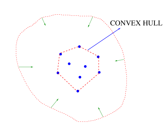
Figure 1: Convex hull of a set of $9$ points obtained by shrinking an elastic, initially stretched outside the set of points, up to the point where it can shrink no more. The resulting final polygon, shown by dotted red line, is the convex hull associated with this set of points.

Properties of convex hulls have been widely studied in mathematics, computer science and also in the physics of crystallography in connection with the so called Wulff construction. Convex hulls are widely used in computer aided image processing, in particular for pattern recognition [1]. Finding efficient algorithms to construct the convex hull of a set of points has led to numerous studies over the last few decades [2, 3, 4, 5, 6, 7]. In addition, convex hulls are used as a standard estimator for the home range for animal movements in ecology, leading to several important practical applications [8, 9, 10]. For a recent review on the history and applications of convex hulls, see Ref. [12].

Of particular interest are the statistical properties of the convex hull associated with a set of random points on the plane. Consider, for instance, the set of $N$ points whose coordinates $\{{\vec{r}_{1}},{\vec{r}_{2}},\ldots,{\vec{r}_{N}}\}$ are random variables drawn, in general, from a joint distribution $P\left({\vec{r}_{1}},{\vec{r}_{2}},\ldots,{\vec{r}_{N}}\right)$. For each realization of the points, one can construct the associated convex hull and compute observables such as the perimeter $L$, area $A$ or the number of vertices $V$ of this convex hull. Clearly these observables change from one realization of points to another and are themselves random variables. Given the underlying distribution of the points $P\left({\vec{r}_{1}},{\vec{r}_{2}},\ldots,{\vec{r}_{N}}\right)$, a challenging hard problem is to compute the statistics of the observables associated with the convex hull, e.g., the distributions such as $P(L)$, $P(A)$ or $P(V)$. Even computing the mean perimeter $\langle L\rangle$ , mean area $\langle A\rangle$ and the mean number of vertices $\langle V\rangle$ on the convex hull is, in general, a hard problem. This is not just a mathematically challenging problem, but has several important practical applications, as reviewed recently in Ref. [12]. While several results are known (see [12] for a review) in the case when the points are distributed independently and identically, i.e., when the joint distribution factorises, $P\left({\vec{r}_{1}},{\vec{r}_{2}},\ldots,{\vec{r}_{N}}\right)=\prod_{i=1}^{N}p(\vec{r}_{i})$, very few results are known when the vertices are correlated.

A classic example when the points are correlated is the case when ${\vec{r}_{i}}$ represents the position of a two-dimensional random walk at time step $i$. Each component of the position of the random walker evolves via the Markov evolution rule

$$x_{i} = x_{i-1}+\eta_{x}(i)$$ (1)

$$y_{i} = y_{i-1}+\eta_{y}(i)$$ (2)

starting from $x_{0}=y_{0}=0$ where the jump lengths $\eta_{x}(i)$ and $\eta_{y}(i)$ in the $x$ and $y$ directions are random variables, independent from each other and are also independent from one step to another and each is a zero mean Gaussian variable with a finite variance $\sigma^{2}$. The walk evolves upto $N$ steps and one can ask, for instance, what is the mean perimeter and the mean area of the convex hull associated with this random walk trajectory? These results are known in the continuous-time limit when $N\to\infty$ and $\sigma^{2}\to 0$ keeping the product $N\sigma^{2}=2DT$ fixed, where $T$ is the total duration of the walk and $D$ is the diffusion constant. In the continuous-time limit, Eqs. (1)-(2) reduce to the Brownian motion in a plane

$$\frac{dx}{dt} = \eta_{x}(t)$$ (3)

$$\frac{dy}{dt} = \eta_{y}(t)$$ (4)

starting at the origin $x(0)=y(0)=0$, and where $\eta_{x}(t)$ and $\eta_{y}(t)$ are Gaussian white noises with zero mean and the two-time correlators, $\langle\eta_{x}(t)\eta_{x}(t^{\prime})\rangle=2D\delta(t-t^{\prime})$, $\langle\eta_{y}(t)\eta_{y}(t^{\prime})\rangle=2D\delta(t-t^{\prime})$ and $\langle\eta_{x}(t)\eta_{y}(t^{\prime})\rangle=0$. In this continuous-time limit, the mean perimeter of the convex hull associated to this Brownian motion of total duration $T$ was first computed by Takács, $\langle L(T)\rangle=\sqrt{16\pi\,D\,T}$ [13]. Note that while the $\sqrt{D\,T}$ dependence of the perimeter is expected due to the diffusive nature of the path, the computation of the prefactor $\sqrt{16\pi}$ is highly nontrivial. Later, the mean perimeter of the convex hull associated with a two dimensional Brownian bridge (where the walker is constrained to come back to the origin after time $T$) was also computed exactly by Goldman, $\langle L(T)\rangle_{\rm bridge}=\sqrt{\pi^{3}DT}$ [14]. The mean area of the convex hull for a free Brownian motion of duration $T$ , $\langle A(T)\rangle=\pi\,D\,T$, was first computed by El Bachir and Letac [15, 16], while the corresponding result for the bridge, $\langle A(T)\rangle_{\rm bridge}=(2\pi/3)\,D\,T$ was computed only very recently [17]. Once again, while the linear $D\,T$ dependence is expected (as the area $A\sim L^{2}$), the prefactors were nontrivial to compute. Moreover, the mean perimeter $\langle L_{n}(T)\rangle=\alpha_{n}\sqrt{D\,T}$ and the mean area $\langle A_{n}(T)\rangle=\beta_{n}(D\,T)$ of the convex hull of $n$ independent two-dimensional Brownian motions each of duration $T$ was exactly computed recently for all $n$ [17, 12] both for free Brownian paths and Brownian bridges and the prefactors $\alpha_{n}$ and $\beta_{n}$ were found to have nontrivial $n$ dependence.

While the positions of a two-dimensional Brownian motion are correlated, the time evolution of the process is still Markovian. An important question is if one can compute the statistics of the convex hull associated to a two-dimensional non-Markovian stochastic process. This would then be a nontrvial generalisation. The purpose of this paper is to present exact analytical results for the mean perimeter and the mean area of the convex hull associated with the trajectory of a two-dimensional non-Markovian stochastic process, namely, the two dimensional random acceleration process. In this process, the position $(x,y)$ of a particle in the plane evolves in continuous-time $t$ via

$$\frac{d^{2}x}{dt^{2}} = \eta_{x}(t)$$ (5)

$$\frac{d^{2}y}{dt^{2}} = \eta_{y}(t)$$ (6)

where $\eta_{x}(t)$ and $\eta_{y}(t)$ are zero mean Gaussian white noises as in Eqs. (3)-(4), with two-point correlators, $\langle\eta_{x}(t)\eta_{x}(t^{\prime})\rangle=2D\delta(t-t^{\prime})$, $\langle\eta_{y}(t)\eta_{y}(t^{\prime})\rangle=2D\delta(t-t^{\prime})$ and $\langle\eta_{x}(t)\eta_{y}(t^{\prime})\rangle=0$. Henceforth, for simplicity, we will set $D=1$ without any loss of generality. Note that due to the presence of the second derivative in Eqs. (5)-(6), the evolution is non-Markovian. If however, one defines the velocities, $v_{x}=dx/dt$ and $v_{y}=dy/dt$, then in the position-velocity phase space, the evolution equation involves only first derivative in time and hence the joint $(\vec{r},\vec{v})$ process becomes Markovian,

$$\frac{dx}{dt} = v_{x}(t);\quad\quad\frac{dv_{x}}{dt}=\eta_{x}(t)$$ (7)

$$\frac{dy}{dt} = v_{y}(t);\quad\quad\frac{dv_{y}}{dt}=\eta_{y}(t).$$ (8)

At time instant $t$ the particle is identified by its position $\vec{r}(t)=(x(t),y(t))$ and its velocity $\vec{v}(t)=\left(v_{x}(t)=dx/dt,v_{y}(t)=dy/dt\right)$. We assume that the particle starts at the origin $(x=0,y=0)$ at time $0$ with initial zero velocities: $(v_{x}(0)=0,v_{y}(0)=0)$. We evolve the process up to time $T$ and then construct the convex hull associated with the trajectory in the $(x-y)$ plane and compute the statistics of observables such as the perimeter $L(T)$, the area $A(T)$ and the number of vertices $V(T)$. A particular realization of this process and the associated convex hull is shown in Fig. (2).

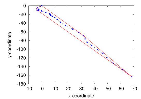
Figure 2: Convex hull of $30$ points generated using the discrete random acceleration process defined in Eqs. (3)-(3). The convex hull is constructed using the Graham span algorithm [2].

Our main results are summarized as follows. We show that the mean perimeter and the mean area of the convex hull associated to a two-dimensional random acceleration process of duration $T$, starting from the initial zero velocity conditions $v_{x}(0)=v_{y}(0)=0$, are given by the following exact expressions

$$\langle L(T)\rangle = \sqrt{\frac{3\pi}{2}}\,T^{3/2}=(2.1708\ldots)\,T^{3/2}$$ (9)

$$\langle A(T)\rangle = \frac{5\pi}{192}\,\sqrt{\frac{3}{2}}\,T^{3}=(0.100199\ldots)\,T^{3}.$$ (10)

As in case of Brownian motion, while the $T$ dependence of the mean perimeter and the mean area easily follow from dimensional grounds, computation of the prefactors turns out to be rather nontrivial and they are the main results of this paper. We could not compute the mean number of vertices analytically, for which we present only numerical results.

The random acceleration process is perhaps the simplest non-Markovian process and hence, no wonder, that it has been intensively studied both in the Physics and the Mathematics literature. Even though it is simple, the first-passage properties of this process are highly nontrivial even in one dimension, though several exact results are known  [18, 19, 20, 21, 22, 23, 24, 25, 27, 28, 29, 30, 26, 31, 32, 33]. There are several applications of this process, notably in the continuum description of semiflexible polymer chain [22], of fluctuating linear interfaces with dynamic exponent $z=4$ [28] and also in the description of the statistical properties of Burgers equation with Brownian initial velocity [34]. Thus, apart from being mathematically interesting, our results in this paper concerning the statistical properties of the convex hull of a two-dimensional random acceleration process are physically relevant in describing the average ‘shape’ of a ideal semi-flexible polymer chain in two dimensions (without the excluded volume interaction and with one end fixed at the origin while the other end is free).

In deriving our exact results, we map the problem of computing the perimeter and the area of the two dimensional random acceleration process to the problem of computing the statistics of extremes of a one dimensional random acceleration process, following the general method introduced recently in [17, 12]. We remark that a similar mapping between the convex hull of a set of independent points drawn from a unit disc and an effective one dimensional random acceleration process was also noticed recently in the context of the so called Sylvester’s question [35]. The Sylvester’s question asks: given a set of $N$ independent points (drawn from a unit disc), what is the probabablity that all $N$ points lie on the convex hull? In other words, in our notation the probability $P(V=N)$ where $V$ is the number of vertices on the convex hull. Based on the mapping to the one dimensional random acceleration process, the authors of Ref. [35] derived exact asymptotic results for $P(V=N)$ for large $N$.

The rest of the paper is organized as follows. In Section 2, we show how one can use Cauchy’s formulae to map the problem of computing the perimeter and the area of the convex hull of a generic two dimensional stochastic process to the problem of computing the moments of the maximum and the time at which the maximum occurs for the associated one dimensional component stochastic process. We then focus on the random acceleration process and show how to compute explicitly the mean perimeter and the mean area of its convex hull using this mapping. In Section 3, we present the results of numerical simulations. We conclude in Section 4 with a summary and open problems. The detailed calculation of the moments of the maximum of a one dimensional random accelertion process, required for our main results, is relegated to the Appendix A.

2 Mapping to the extreme value statistics of a one dimensional process using Cauchy’s formulae

In Refs. [17, 12] it was shown that the problem of computing the perimeter and the area of the convex hull of any two dimensional stochastic process $[x(t),y(t)]$ can be mapped to computing the statistics of the value of the maximum and the time of occurrence of the maximum of the one dimensional component process $x(t)$. This was achieved in [17, 12] by exploiting the formulae for the perimeter and the area of any arbitrary closed, convex curve in two dimensions, derived originally by Cauchy [36]. We start this section by briefly reviewing this useful mapping and then use this mapping to compute explicitly the mean perimeter and the mean area of the convex hull of the two dimensional random acceleration process defined in Eqs. (5)-(6).

Consider any closed convex curve $C$ on a plane (see Fig. 3). We choose the coordinate system such that the origin is inside the curve $C$. A key quantity, introduced by Cauchy [36], is the so called support function. Consider any direction $\theta$. For fixed $\theta$, consider a stick perpendicular to this direction and imagine bringing the stick from infinity and stop when it first touches the curve $C$ (see Fig. 3). At this point, the distance $M(\theta)$ of the stick from the origin is called the support function in the direction $\theta$. It is clearly a very intuitive quantity as it measures how close can one get to the curve $C$ in the direction $\theta$ coming from infinity. Mathematically speaking, consider all points on the curve $C$ with coordinates $[X(s),Y(s)]$ (where $s$ is the distance measured along the curve that just parametrizes the curve), consider their projections in the direction $\theta$ and then compute the maximum projection, i.e.,

$$M(\theta)=\max_{s\in C}\left[X(s)\cos(\theta)+Y(s)\sin(\theta)\right].$$ (11)

Once this support function $M(\theta)$ is known, then the perimeter $L$ of $C$ and the area $A$ enclosed by $C$ are given by Cauchy’s formulae [36]

$$L = \int_{0}^{2\pi}M(\theta)\,d\theta$$ (12)

$$A = \frac{1}{2}\int_{0}^{2\pi}\left[M^{2}(\theta)-(M^{\prime}(\theta))^{2}\right]\,d\theta$$ (13)

where $M^{\prime}(\theta)=dM/d\theta$. For example, for a circle of radius $R=r$, $M(\theta)=r$ and one recovers the standard formulae: $L=2\pi r$ and $A=\pi r^{2}$. The formulae in Eqs. (12)-(13) are generalisations of the circle formulae, valid for arbitrary closed convex curve $C$. A simple proof of the formulae can be found in the Appendix A of Ref. [12].

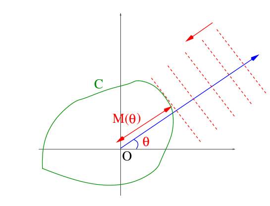
Figure 3: Support function $M(\theta)$ in the direction $\theta$ for a closed convex curve $C$ on a plane.

Now, consider any two dimensional stochastic process $[x(t),y(t)]$ up to time $T$, starting from $[x(0)=0,y(0)=0]$. For every realization, i.e., for every trajectory of the process, let us construct the corresponding convex hull $C$, which clearly varies from one trajectory to another. The idea then is to apply the Cauchy’s formulae to each of these closed convex curves $C$ and then average over all realizations to compute the mean perimeter and the mean area. To apply Cauchy’s formulae to a particular convex hull $C$, we need to first compute its associated support function $M(\theta)$ defined in Eq. (11). It looks rather complicated to first compute the locus $[X(s),Y(s)]$ of the convex hull and then maximize over $s$. However, the crucial point to realize [17, 12] is that $M(\theta)$ represents the maximum projection of the convex hull $C$ in the direction $\theta$, which is also precisely the maximum projection of the trajectory $[x(t),y(t)]$ itself in the direction $\theta$, i.e.,

$$M(\theta) = \max_{s\in C}\left[X(s)\cos(\theta)+Y(s)\sin(\theta)\right]$$ (14)

$$= \max_{0\leq t\leq T}\left[x(t)\cos(\theta)+y(t)\sin(\theta)\right].$$

So, in principle, if we have the list of cordinates visited by the trajectory up to time $T$, we can compute the support function $M(\theta)$ by maximizing over time $t$. Let us denote $z_{\theta}(t)=x(t)\cos(\theta)+y(t)\sin(\theta)$. For a fixed $\theta$, $z_{\theta}(t)$ is just a one dimensional process parametrized by $\theta$. Thus the support function $M(\theta)$ is just the maximum of this one dimensional process $z_{\theta}(t)$ over the time interval $t\in[0,T]$. Furthermore, assuming that the maximum of $z_{\theta}(t)$ (with $0\leq t\leq T$) occurs at time $t_{m}$, we have

$$M(\theta)=\max_{0\leq t\leq T}\left[z_{\theta}(t)\right]=z_{\theta}(t_{m})=x(t_{m})\cos(\theta)+y(t_{m})\sin(\theta).$$ (15)

where $t_{m}$ implicitly depends on $\theta$. The derivative $M^{\prime}(\theta)$ needed in the area formula in Eq. (13) can then be computed by deriving the right hand side (r.h.s) of Eq. (15) with respect to $\theta$. This gives

$$M^{\prime}(\theta)=-x(t_{m})\sin(\theta)+y(t_{m})\cos(\theta)+\frac{dt_{m}}{d\theta}\,\frac{dz_{\theta}(t)}{dt}\Big{|}_{t=t_{m}}.$$ (16)

However, since $z_{\theta}(t)$ is maximum at $t=t_{m}$, by definition, $dz_{\theta}(t)/dt|_{t=t_{m}}=0$ and hence the last term on the r.h.s vanishes and one simply gets

$$M^{\prime}(\theta)=-x(t_{m})\sin(\theta)+y(t_{m})\cos(\theta).$$ (17)

The equations (15) and (17) are the essential ingredients behind the mapping of the original two dimensional convex hull problem to the statistics of the maximum of an effective one dimensional process. Now, an additional simplicity can arise if the two dimensional stochastic process is rotationally invariant, as in the case of Brownian motion and also for the random acceleration process. In this case, any average over the realizations is independent of the angle $\theta$. Thus, the integral $I=\int_{0}^{2\pi}\langle F[M(\theta)]\rangle\,d\theta$ just reduces, thanks to the isotropy, to $I=2\pi\langle F[M(0)]\rangle$, for any function $F[M]$. Setting $\theta=0$ in Eqs. (15) and (17) we note that

$$M(0) = x(t_{m})=m(T)$$ (18)

$$M^{\prime}(0) = y(t_{m})$$ (19)

where $m(T)$ denotes the maximum of the one dimensional component process $x(t)$ over the interval $0\leq t\leq T$ and $t_{m}$ denotes the time at which $x(t)$ achieves its maximum. On the other hand $M^{\prime}(0)$ is the value of the other independent one dimensional process $y(t)$ at the time $t=t_{m}$ when the first process $x(t)$ attains its maximum (see Fig. (4)).

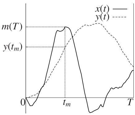
Figure 4: Schematic picture of $m(T)$, $t_{m}$ and $y(t_{m})$.

Thus, the mean perimeter and the mean area, taking average over Cauchy’s formulae, using isotropy, and Eqs. (18) and (19), are simply given by

$$\langle L(T)\rangle = 2\pi\,\langle M(0)\rangle=2\pi\langle m(T)\rangle$$ (20)

$$\langle A(T)\rangle = \pi\left[\langle M^{2}(0)\rangle-\langle(M^{\prime}(0))^{2}\rangle\right]=\pi\left[\langle m^{2}(T)\rangle-\langle y^{2}(t_{m})\rangle\right]$$ (21)

So far, the results in Eqs. (20) and (21) are quite general and hold for any arbitrary two dimensional rotationally invariant stochastic process $[x(t),y(t)]$. To compute the mean perimeter and the mean area, we then need to compute three quantities for the associated one dimensional component process $x(t)$, namely the first two moments of the maximum $m(T)$ of the one dimensional process $x(t)$ over the interval $0\leq t\leq T$: (i) $\langle m(T)\rangle$ (ii) $\langle m^{2}(T)\rangle$ and also (iii) $\langle y^{2}(t_{m})\rangle$ where $t_{m}$ is the time at which the process $x(t)$ attains its maximum value. For the Brownian motion, these three quantities can be easily calculated [17, 12]. Here we show that for the random acceleration process as well, one can compute these three quantities explicitly.

For a one dimensional random acceleration process $x(t)$, evolving via $d^{2}x/dt^{2}=\eta_{x}(t)$, over the interval $0\leq t\leq T$, the Laplace transform of the distribution of the maximum was obtained recently by Burkhardt [32]. This Laplace transform has a rather complicated form (expressed as an integral over Airy function) (see Eq. (A.4) in Appendix A). Computing explicitly the moments of $m(T)$ from this Laplace transform turns out to be rather nontrivial. However, fortunately this can be done as we show in Appendix A. In particular, for the first two moments, we get

$$\langle m(T)\rangle=\sqrt{\frac{3}{8\pi}}\,T^{3/2}$$ (22)

$$\langle m^{2}(T)\rangle=\left(\frac{2}{3}-\frac{103}{384}\sqrt{\frac{3}{2}}\right)\,T^{3}.$$ (23)

Finally, it rests to compute $\langle y^{2}(t_{m})\rangle$. This can be done in two steps. First, we note from the evolution equation, $d^{2}y/dt^{2}=\eta_{y}(t)$ [where $\langle\eta_{y}(t)\rangle=0$ and $\langle\eta_{y}(t)\eta_{y}(t^{\prime})\rangle=2\delta(t-t^{\prime})$], that at any fixed time $t$, $\langle y^{2}(t)\rangle=(2/3)\,t^{3}$ for all $t$. This is easily obtained by integrating the evolution equation and computing $\langle y^{2}(t)\rangle$ using the delta correlation of the noise. Secondly, averaging over the distribution $p(t_{m}|T)$ of the time of the maximum $t_{m}$ of $x(t)$ one gets

$$\langle y^{2}(t_{m})\rangle=\frac{2}{3}\langle t_{m}^{3}\rangle=\frac{2}{3}\,\int_{0}^{T}dt_{m}\,t_{m}^{3}\,p(t_{m}|T).$$ (24)

So, we need to know the distribution $p(t_{m}|T)$ of the time $t_{m}$ at which a random acceleration process achieves its maximum over the interval $t\in[0,T]$. Fortunately, this is exactly known from our recent calculation [33]

$$p(t_{m}|T)=C\,\delta(T-t_{m})+\frac{(1-C)}{\pi\sqrt{2}}t_{m}^{-3/4}\,(T-t_{m})^{-1/4},$$ (25)

where the constant $C$ has the exact value

$$C=1-\sqrt{\frac{3}{8}}=0.387628\ldots$$ (26)

Using this result in Eq. (24) we finally get

$$\langle y^{2}(t_{m})\rangle=\frac{2}{3}\left(C+\frac{15}{128}(1-C)\right)T^{3}=\left(\frac{2}{3}-\frac{113}{384}\sqrt{\frac{3}{2}}\right)T^{3}.$$ (27)

Substituting the results from Eqs. (22), (23) and (27) in Eqs. (20) and (21) immediately gives our main results

$$\langle L(T)\rangle = \sqrt{\frac{3\pi}{2}}\,T^{3/2}=(2.1708\ldots)\,T^{3/2}$$ (28)

$$\langle A(T)\rangle = \frac{5\pi}{192}\,\sqrt{\frac{3}{2}}\,T^{3}=(0.100199\ldots)\,T^{3}.$$ (29)

3 Numerical simulations

To verify our main theoretical predictions, we have also performed simulations of a discrete version of the random acceleration process in two dimensions. A particle at discrete time, $n=0,1,\ldots,N$, is identified by its position $(x(n),\,y(n))$ and its velocity $(v_{x}(n),\,v_{y}(n))$. At time $n+1$ the velocity is updated by the discrete-time version of the Markov evolution rules in Eqs. (7) and (8):

$$v_{x}(n) = v_{x}(n-1)+\eta_{x}(n)$$

$$v_{y}(n) = v_{y}(n-1)+\eta_{y}(n)$$ (30)

where $\eta_{x}(n),\eta_{y}(n)$ are uncorrelated Gaussian normal variables each with zero mean and variance $\sigma^{2}=2$. The position $(x(n),\,y(n))$ is then updated:

$$x(n) = x(n-1)+v_{x}(n)$$

$$y(n) = y(n-1)+v_{y}(n)$$ (31)

The process is started from $x(0)=y(0)=v_{x}(0)=v_{y}(0)=0$ and iterated for $N-1$ steps and then the convex hull is constructed using the Graham scan algorithm [2]. An example is shown in Fig. (2). The output of each realization is the ordered set of the $V$ vertices sorted clockwise from $(x_{1},y_{1})$ to $(x_{V},y_{V})$. The perimeter and the area of the convex hull can then be computed using the formulae:

$$L=\sum_{i=1}^{V}\sqrt{(x_{i+1}-x_{i})^{2}+(y_{i+1}-y_{i})^{2}}$$ (32)

$$A=-\frac{1}{2}\sum_{i=1}^{V}\left(x_{i}y_{i+1}-x_{i+1}y_{i}\right)$$ (33)

where we assume $x_{V+1}=x_{1}$ and $y_{V+1}=y_{1}$. It is important to note that the minus symbol in Eq. (33) is due to the clockwise sorting of the points: indeed, the area formula (commonly called the surveyor’s formula) gives the algebrical value of the area of a polygon; it gives the real area if the points are sorted counterclockwise, which is not the case here.

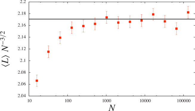
Figure 5: Behavior of $\langle L\rangle$. Symbols: numerical data for the model defined by Eqs. (3) and (3). Solid line: continuum model prediction, $\sqrt{3\pi/2}\sim 2.1708038\ldots$.

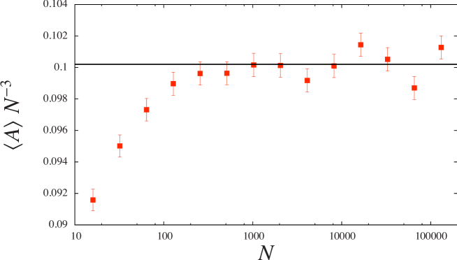
Figure 6: Behavior of $\langle A\rangle$. Symbols: numerical data for the model defined by Eqs. (3) and (3). Solid line: continuum model prediction, $5\pi\sqrt{3/2}/192\sim 0.10019921\ldots$.

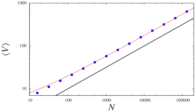
Figure 7: Behavior of $\langle V\rangle$. Symbols: numerical data for the model defined by Eqs. (3) and (3). Solid line: scaling behavior $\sim\sqrt{N}$. Dashed line: best fit.

The perimeter $L$, the area $A$ and the number of vertices $V$ are stochastic variables which fluctuate from one realization to another. We computed $\langle L\rangle$, $\langle A\rangle$, $\langle V\rangle$ for different values of $N$. For each $N$, we average over $10^{4}$ realizations. For large $N$, the leading asymptotic behaviors of the mean perimeter and the mean area should be given by the continuous-time limit results in Eqs. (28) and (29)

$$\langle L\rangle = \sqrt{\frac{3\pi}{2}}\,N^{3/2}+O(N)$$ (34)

$$\langle A\rangle = \frac{5\pi}{192}\,\sqrt{\frac{3}{2}}\,N^{3}+O(N^{5/2}).$$ (35)

In Figs. (5) and (6), we present our data respectively for the average perimeter $\langle L\rangle$ and the average area $\langle A\rangle$ of the convex hull, as a function of $N$. Both the scaling and the numerical prefactor of the leading behavior in $N$ are recovered. The agreement between the simulation and the analytical results is excellent.

Furthermore, something rather interesting can be remarked on Fig. 7. For large $N$, the leading behavior of the average number of vertices seems to be $\langle V\rangle\sim\sqrt{N}$. Numerically we find

$$\langle V\rangle\sim c_{1}\sqrt{N}+c_{2}+O(1/\sqrt{(}N)).$$ (36)

A best fit gives $c_{1}=1.735\pm 0.01$ and $c_{2}=2.6\pm 1.0$. We were not able to derive this result analytically and it remains an interesting open question.

4 Summary and Conclusion

In summary, in this paper we have computed analytically the mean perimeter $\langle L(T)\rangle$ and the mean area $\langle A(T)\rangle$ of the convex hull of a two dimensional random acceleration process of duration $T$, starting at the origin with zero initial velocity. We have used an exact mapping, via Cauchy’s formulae, that relates the computation of the perimeter and the area of the convex hull of a two dimensional stochastic process to computing the extremal statistics associated with the corresponding one dimensional component stochastic process. Physically our results describe the average shape of a semi-flexible ideal polymer chain in two dimensions.

We have also presented numerical results that suggest that the mean number of vertices $V$ of the convex hull associated to the discrete-time version of the random acceleration process up to $N$ steps scales as $\langle V(N)\rangle\approx c_{1}\sqrt{N}+c_{2}+O(1/\sqrt{N})$ for large $N$. Proving this result and the computation of the constants $c_{1}$ and $c_{2}$ remain a challenging open problem.

It is interesting to compare our exact results for the convex hull associated with a two-dimensional random acceleration process with those for the convex hull assocaited to a planar Brownian motion. In particular one notes that the ratio $r=\langle A\rangle/{\langle L\rangle}^{2}$ has very different values for the two processes. For a random acceleration process, using our exact results in Eqs. (9) and (10), we get $r=(5/192)\sqrt{2/3}=0.02126\dots$. The corresponding ratio for a free Brownian motion, using results mentioned in the introduction, is $r=1/16=0.0625$ which is larger than the random acceleration process. The geometrical implication of this result is that the convex hull associated with the Brownian motion is, roughly speaking, more space filling than the one associated with the random acceleration process. In the latter case, the convex hull tends to be more ‘elongated’ as evident from a typical representation in Fig. (2). This is somewhat expected from the statistical mechanical consideration of the semi-flexible polymer chains described by the random acceleration process: the typical configuration of such a curvature-driven chain tends to be elongated as it costs more energy to bend or curve them as compared to a typical Brownian trajectory of a Rouse chain.

There are several directions in which our work can be possibly extended. In this paper, we managed to compute only the mean perimeter and the mean area of the convex hull of the random acceleration process. It remains a challenging problem to compute the fluctuations or even the full distribution of these observables associated with the convex hull of the random acceleration process. The mapping we discussed in this paper is quite general and holds for arbitrary two dimensional stochastic process. It would be interesting to exploit this mapping to compute the mean perimeter and the mean area of the convex hull of other interesting two dimensional non-Markovian stochastic processes. For instance, for the process $d^{n}\vec{r}/dt^{n}=\vec{\eta}(t)$ (where $n=1$ and $n=2$ correspond respectively to the Brownian motion and the random acceleration process) with $n>2$, it would be interesting to see if one can compute the statistics of the associated convex hulls.

Appendix A The moments of the maximum value distribution

Consider a one dimensional random acceleration process $x(t)$ in the time interval $[0,T]$. At time $t=0$ the process starts from $x_{0}=0$ with zero velocity, $v_{0}=0$. Let $m(T)$ denote the global maximum value achieved by $x(t)$ during the interval $[0,T]$. We wish to compute the cumulative probability distribution of the maximum, i.e., ${\rm Prob}\left[m(T)<z\right]$. Clearly, this is the probability that the value of the process, starting initially at $x=0$, does not exceed the level $z$. In other words, ${\rm Prob}\left[m(T)<z\right]={\rm Prob}\left[x(t)<z,\,\,{\rm for\,\,all\,\,0\leq t\leq T}\right]$. We then introduce the change of variable $\tilde{x}(t)=z-x(t)$. The process $\tilde{x}(t)$ is also a random acceleration process, starting from $z$ (with zero velocity). The probability that $m(T)$ is smaller than $z$ can then be expressed in terms of the survival probability of the new process $\tilde{x}(t)$, i.e., the probability $q(z,0,T)$ that the process $\tilde{x}(t)$ stays positive over the initerval $t\in[0,T]$ given that it started from the initial value $\tilde{x}(0)=z$. We then write

$$\mbox{Prob}\left[m(T)<z\right]=\mbox{Prob}\left[\{x(t)\}<z\right]=\mbox{Prob}\left[\{\tilde{x}(t)\}>0\right]=q(z,0,T).$$ (37)

Note that $q(0,0,T)=0$ and $q(z\to\infty,0,T)=1$.

The moments of the maximum $m$ can be expressed in terms of the survival probability:

$$\langle m^{n}(T)\rangle=\int_{0}^{\infty}dz\,z^{n}\frac{dq}{dz}=-\int_{0}^{\infty}dz\,z^{n}\frac{d}{dz}\left[1-q\right]=n\int_{0}^{\infty}dz\,z^{n-1}\left[1-q(z,0,T)\right]$$ (38)

where we have used integration by parts and the boundary condition $q(z\to\infty,0,T)=1$. Let $\tilde{q}(z,0,s)$ denote the Laplace transform of the survival porbability:

$$\tilde{q}(z,0,s)=\int_{0}^{\infty}dT\,e^{-sT}\,q(z,0,T).$$ (39)

This quantity can be expressed as an integral [22, 32]:

$$\frac{1}{s}-\tilde{q}(z,0,s)=\int_{0}^{\infty}\frac{dF}{F^{5/3}}\,e^{-Fz}\mbox{Ai}\left(\frac{s}{F^{2/3}}\right)\left[1+\frac{\Gamma\left(-\frac{1}{2},\frac{2}{3}\frac{s^{3/2}}{F}\right)}{4\sqrt{\pi}}\right],$$ (40)

where $\Gamma\left(-\frac{1}{2},y\right)$ is the incomplete Gamma function. We can thus introduce the Laplace transform of the moments in Eq. (38) and obtain

$$\int_{0}^{\infty}dT\,e^{-sT}\,\langle m^{n}(T)\rangle=n\int_{0}^{\infty}dz\,z^{n-1}\int_{0}^{\infty}\frac{dF}{F^{5/3}}\,e^{-Fz}\mbox{Ai}\left(\frac{s}{F^{2/3}}\right)\left[1+\frac{\Gamma\left(-\frac{1}{2},\frac{2}{3}\frac{s^{3/2}}{F}\right)}{4\sqrt{\pi}}\right].$$

Performing the integral over $z$ we get

$$\int_{0}^{\infty}dT\,e^{-sT}\,\langle m^{n}(T)\rangle=\Gamma(n+1)\int_{0}^{\infty}\frac{dF}{F^{5/3+n}}\,\mbox{Ai}\left(\frac{s}{F^{2/3}}\right)\left[1+\frac{\Gamma\left(-\frac{1}{2},\frac{2}{3}\frac{s^{3/2}}{F}\right)}{4\sqrt{\pi}}\right].$$

Next we introduce a change of variable $y=2s^{3/2}/(3F)$,

$$\int_{0}^{\infty}dT\,e^{-sT}\,\langle m^{n}(T)\rangle=\frac{\Gamma(n+1)}{s^{\frac{3}{2}n+1}}\left(\frac{3}{2}\right)^{n+\frac{2}{3}}\int_{0}^{\infty}dyy^{n-\frac{1}{3}}\,\mbox{Ai}\left[\left(\frac{3y}{2}\right)^{2/3}\right]\left[1+\frac{\Gamma\left(-\frac{1}{2},y\right)}{4\sqrt{\pi}}\right].$$

As a result, the $s$ dependence of the r.h.s is very simple, just proportional to $s^{-3n/2-1}$ and hence its inverse Laplace transform (with respect to $s$) can be done trivially to give

$$\langle m^{n}(T)\rangle=\left\{\left(\frac{3}{2}\right)^{n-\frac{1}{3}}\frac{\Gamma(n)}{\Gamma(\frac{3}{2}n)}\int_{0}^{\infty}dy\,y^{n-\frac{1}{3}}\,\mbox{Ai}\left[\left(\frac{3y}{2}\right)^{2/3}\right]\left[1+\frac{\Gamma\left(-\frac{1}{2},y\right)}{4\sqrt{\pi}}\right]\right\}T^{\frac{3}{2}n}.$$ (41)

At this point, it turns out to be useful to express the Airy function in terms of the modified Bessel function $K_{\nu}(z)$ using the following identity [37]:

$$\mbox{Ai}\left[\left(\frac{3y}{2}\right)^{2/3}\right]=\frac{1}{\sqrt{3}\pi}\left(\frac{3}{2}\right)^{\frac{1}{3}}\,y^{1/3}\,\mbox{K}_{\frac{1}{3}}(y).$$ (42)

Then we have

$$\langle m^{n}(T)\rangle=\left(\frac{3}{2}\right)^{n}\frac{\Gamma(n)}{\sqrt{3}\pi\Gamma(\frac{3}{2}n)}\,I^{(n)}\,T^{\frac{3}{2}n}$$ (43)

where

$$I^{(n)}=\int_{0}^{\infty}dy\,y^{n}\,\mbox{K}_{\frac{1}{3}}(y)\left[1+\frac{\Gamma\left(-\frac{1}{2},y\right)}{4\sqrt{\pi}}\right].$$ (44)

We now show that the integral $I^{(n)}$ can be computed for any non-negative integer $n$. Starting from the definition of the incomplete $\Gamma$ function, $\Gamma\left(\alpha,y\right)=\int_{y}^{\infty}dt\,t^{\alpha+1}\,e^{-t}$, we first use the following decomposition formula valid for any non-negative integer $n$,

$$\frac{\Gamma\left(-\frac{1}{2},y\right)}{4\sqrt{\pi}}=\frac{1}{2\pi}\left[(-1)^{n}\Gamma(n+\frac{3}{2})\Gamma(-n-\frac{1}{2},y)-e^{-y}\sum_{k=1}^{n}(-1)^{k}\frac{\Gamma(k+\frac{1}{2})}{y^{k+\frac{1}{2}}}\right],$$ (45)

which can be easily obtained by repeated integration by parts. We then split the main integral $I^{(n)}$ into three parts $I^{(n)}=I_{1}+I_{2}+I_{3}$ with

$$I_{1}=\int_{0}^{\infty}\,dy\,y^{n}\mbox{K}_{\frac{1}{3}}(y)$$

$$I_{2}=(-1)^{n}\Gamma(n+\frac{3}{2})\int_{0}^{\infty}\frac{dy}{2\pi}\,y^{n}\,\mbox{K}_{\frac{1}{3}}(y)\Gamma(-n-\frac{1}{2},y)$$

$$I_{3}=-\sum_{k=1}^{n}(-1)^{k}\Gamma(k+\frac{1}{2})\int_{0}^{\infty}\frac{dy}{2\pi}\,y^{n-k-\frac{1}{2}}\,e^{-y}\,\mbox{K}_{\frac{1}{3}}(y)$$ (46)

A.0.1 Evaluation of $I_{2}$

Using the identity [37],

$$\Gamma(n+\frac{3}{2})\Gamma(-n-\frac{1}{2},y)=\frac{e^{-y}}{y^{n+1/2}}\int_{0}^{\infty}\,dt\,\frac{e^{-t}t^{n+1/2}}{t+y},$$

and the formula [37],

$$\int_{0}^{\infty}\frac{dy}{\sqrt{y}}\frac{e^{-y}\mbox{K}_{\nu}(y)}{y+t}=\frac{\pi\,e^{t}\,\mbox{K}_{\frac{1}{3}}(t)}{\sqrt{t}\cos(\nu\pi)},$$

$I_{2}$ can be recast:

$$I_{2}=(-1)^{n}\int_{0}^{\infty}\,dt\,e^{-t}t^{n+1/2}\int_{0}^{\infty}\frac{dy}{2\pi\sqrt{y}}\,\frac{e^{-y}}{t+y}\,\mbox{K}_{\frac{1}{3}}(y)$$

and the integral over $y$ can be performed

$$I_{2}=(-1)^{n}\int_{0}^{\infty}\,dt\,t^{n}\mbox{K}_{\frac{1}{3}}(t)=(-1)^{n}I_{1}$$

A.1 Evaluation of $I_{1}$

The integral $I_{1}$ can be computed [37]

$$I_{1}=\sqrt{3}\pi\left(\frac{2}{3}\right)^{n}\frac{\Gamma(\frac{3}{2}n)}{\sqrt{3^{n}}\Gamma(\frac{1}{2}n)}$$

A.1.1 Evaluation of $I_{3}$

Using the integral [37]

$$\int_{0}^{\infty}dy\,y^{\mu-1}\,e^{-y}\,\mbox{K}_{\frac{1}{3}}(y)=\frac{\sqrt{\pi}}{2^{\mu}}\frac{\Gamma(\mu+1/3)\Gamma(\mu-1/3)}{\Gamma(\mu+1/2)}$$

with $\mu=n-k+1/2$ and the change of variable $j=n-k$ we get

$$I_{3}=\frac{(-1)^{n-1}}{\sqrt{8\pi}}S_{n}$$

where

$$S_{n}=\sum_{j=0}^{n-1}\frac{\Gamma(j+5/6)\Gamma(j+1/6)\Gamma(n-j+\frac{1}{2})}{(-2)^{j}\Gamma(j+1)}.$$ (47)

This sum can be performed using Mathematica but it gives a rather cumbersome expression. Hence we prefer to keep this as a discrete sum in Eq. (47).

A.2 The final result

Putting together all these integrals in Eq. (43) we get

$$\langle m^{n}(T)\rangle=\left[\frac{(-1)^{n}+1}{3^{\frac{n}{2}}}\frac{\Gamma(n)}{\Gamma(\frac{n}{2})}-\frac{1}{\sqrt{24\pi^{3}}}\left(-\frac{3}{2}\right)^{n}\frac{\Gamma(n)}{\Gamma(\frac{3}{2}n)}S_{n}\right]T^{\frac{3n}{2}}$$ (48)

where $S_{n}$ is given in Eq. (47). For example, for the first four moments are given explicitly by

$$\langle m(T)\rangle=\sqrt{\frac{3}{8\pi}}\,T^{\frac{3}{2}}$$ (49)

$$\langle m^{2}(T)\rangle=\left(\frac{2}{3}-\frac{103}{384}\sqrt{\frac{3}{2}}\right)\,T^{3}$$ (50)

$$\langle m^{3}(T)\rangle=\frac{1091}{864}\,\sqrt{\frac{3}{8\pi}}\,T^{\frac{5}{2}}$$ (51)

$$\langle m^{4}(T)\rangle=\left(\frac{4}{3}-\frac{5769947}{10616832}\sqrt{\frac{3}{2}}\right)\,\,T^{5}.$$ (52)

References

References

- [1] S. Akl and G. Toussaint, Efficient convex hull algorithms for pattern recognition applications, International Conference on Pattern Recognition, 483 (1978).
- [2] R. Graham, Inf. Process. Lett. 1, 132-133 (1972).
- [3] R. A. Jarvis, Inf. Process. Lett. 2, 18 (1973).
- [4] W. Eddy, ACM Trans. Math. Softw. 3(4), 398 (1977).
- [5] L. Devroye, Comput. Math. Appl. 7, 299 (1981).
- [6] D. G. Kirkpatrick and R. Seidel, SIAM J. Comput. 15 (1), 287 (1986).
- [7] R. Wenger, Algorithmica 17, 322 (1997).
- [8] N. M. Sirakov, J. Math. Imaging Vis. 26(3),309 (2006).
- [9] B. J. Worton, Biometrics 51(4), 1206 (1995).
- [10] L. Giuggioli, G. Abramson, V.M. Kenkre, R.R. Permenter, T.L. Yates, J. Theor. Biol. 240, 126 (2006).
- [11] G. Baxter, Ann. Math. Stat. 32(3), 901 (1961).
- [12] S.N. Majumdar, A. Comtet and J. Randon-Furling, J. Stat. Phys. 138, 955 (2010).
- [13] L. Takács, Am. Math. Mon. 87, 142 (1980).
- [14] A. Goldman, Probab. Theory Relat. Fields 105, 57 (1996).
- [15] M. El Bachir, Ph.D. thesis, Université Paul Sabatier, Toulouse, France (1983).
- [16] G. Letac, J. Theor. Probab. 6, 385 (1993).
- [17] J. Randon-Furling, S. N. Majumdar, and A. Comtet, Phys. Rev. Lett. 103, 140602 (2009).
- [18] H. P. McKean, J. Math. Kyoto Univ. 2 227 (1963).
- [19] M. Goldman, Ann. Math. Stat. 42 2150 (1971).
- [20] T. W. Marshall, E. J. Watson, J. Phys. A: Math. Gen. 18, 3531 (1985).
- [21] Ya. G. Sinai, Theor. Math. Phys. 90, 219 (1992).
- [22] T. W. Burkhardt, J. Phys. A: Math. Gen. 26, L1157 (1993).
- [23] A. Lachal, Stoch. Proc. Appl. 49, 57 (1994).
- [24] S. N. Majumdar, A. J. Bray, Phys. Rev. Lett. 81, 2626 (1998).
- [25] T. W. Burkhardt, J. Phys. A: Math. Gen. 33, L429 (2000).
- [26] T. W. Burkhardt, Phys. Rev. E 63, 011111 (2001).
- [27] G. De Smedt, C. Godreche, J. M. Luck, Europhys. Lett. 53, 438 (2001).
- [28] S. N. Majumdar, A. J. Bray, Phys. Rev. Lett. 86, 3700 (2001).
- [29] G. Gyorgyi, N. R. Moloney, K. Ozogany, Z. Racz, Phys. Rev. E 75, 021123 (2007).
- [30] G. Schehr and S. N. Majumdar, Phys. Rev. Lett. 99, 060603 (2007).
- [31] T. W. Burkhardt, G. Gyorgyi, N. R. Moloney, Z. Racz, Phys. Rev. E 76, 041119 (2007).
- [32] T. W. Burkhardt, J. Stat. Phys. 133, 217 (2008).
- [33] S. N. Majumdar, A. Rosso, and A. Zoia, J. Phys. A: Math. Theor. 43, 115001 (2010).
- [34] P. Valageas, J. Stat. Phys. 134, 589 (2009).
- [35] H. J. Hilhorst, P. Calka, and G. Schehr, J. Stat. Mech.: Theor. and Exp. P10010 (2008).
- [36] A. Cauchy, Mem. Acad. Sci. Inst. Fr. 22, 3 (1850); see also the book by L. A. Santaló, Integral Geometry and Geometric Probability (addison-Wesley, Reading, MA, 1976).
- [37] I. S. Gradshteyn, I. M. Ryzhik, Tables of Integrals, Series, and Products (Academic, New York (1980)).