Localized states on triangular traps and low-temperature properties of the antiferromagnetic Heisenberg and repulsive Hubbard models

Abstract

We consider the antiferromagnetic Heisenberg and the repulsive Hubbard model on two $N$-site one-dimensional lattices, which support dispersionless one-particle states corresponding to localized states on triangular trapping cells. We calculate the degeneracy of the ground states in the subspaces with $n\leq n_{\max}$, $n_{\max}\propto N$ magnons or electrons as well as the contribution of these states (independent localized states) to thermodynamic quantities. Moreover, we discuss another class of low-lying eigenstates (so-called interacting localized states) and calculate their contribution to the partition function. We also discuss the effect of extra interactions, which lift the degeneracy present due to the chirality of the localized states on triangles. The localized states set an extra low-energy scale in the system and lead to a nonzero residual ground-state entropy and to one (or more) additional low-temperature peak(s) in the specific heat. Low-energy degrees of freedom in the presence of perturbations removing degeneracy owing to the chirality can be described in terms of an effective (pseudo)spin-1/2 transverse $XX$ chain.

I Introduction

The thermodynamics of strongly correlated lattice models is generally unknown. Although analytical (like conventional Green’s function technique, dynamical mean-field theory etc) and numerical (like series expansions, quantum Monte Carlo algorithms, density-matrix renormalization group algorithms etc) methods being applied appropriately in particular cases may yield desired thermodynamic characteristics with required accuracy, seeking for new approaches permanently attracts much attention of theoreticians. One interesting idea for calculating thermodynamic quantities for strongly correlated systems, which is related to the concept of localized one-particle states,mielke ; lm has been suggested recently for some spinlocalized_magnons_a ; localized_magnons_b and electronlocalized_electrons models. The localized nature of one-particle states for certain classes of lattices allows to construct exactly the relevant many-particle states and to estimate their contribution to thermodynamics using classical lattice-gas models which are much easier to investigate than the initial quantum many-body models.

In previous investigations of localized states performed for the antiferromagnetic Heisenberg and the repulsive Hubbard model on highly frustrated latticesmielke ; lm ; localized_magnons_a ; localized_magnons_b ; localized_electrons mainly bipartite trapping cells (e.g., a single bond or equilateral even polygons) were considered. These cells have a nondegenerate ground state for the one-particle problem. Here we extend the discussion of localized states to highly frustrated lattices with non-bipartite triangular trapping cells. A non-bipartite cell may have a degenerate ground state for the one-particle problem that may lead to new effects. For example, an equilateral triangle has a two-fold degenerate one-particle ground state, which can be related to the chirality degrees of freedom associated to a triangle, see, e.g., Ref. chirality-parameter, . To be specific, we consider (i) a one-dimensional (1D) lattice which consists of corner sharing “double-tetrahedra” (the double-tetrahedra chain) and (ii) a frustrated (cylindrical) three-leg ladder having a triangular arrangement of rungs (the frustrated triangular tube), cf. Fig. 1. Both lattice geometries have been considered in the literature, see, e.g., Refs. mambrini, ; rojas, ; batista, ; antonosyan, for the double-tetrahedra chain and Refs. subrahmanyam, ; andreas, ; luescher, ; tube_schnack, ; FLP:PRB06, ; nedko, ; sakai, ; penc, for the triangular tube. Note that triangular-tube geometry is realized for the copper spins in [(CuCl₂tachH)₃Cl]Cl₂.tube_schnack ; nedko

In what follows we consider two concrete models of strongly correlated systems on these lattices, namely the spin-1/2 Heisenberg model and the Hubbard model, and discuss the consequences of the localized-magnon or localized-electron states in combination with the additional chirality degrees of freedom. We mention that some similar ideas have been elaborated recently for the Hubbard model on decorated lattices,batista for the coupled tetrahedral Heisenberg chainmambrini ; rojas as well as for the frustrated Heisenberg spin tube.andreas However, in these references the concept of localized states has not been used to discuss low-temperature thermodynamics for thermodynamically large systems. Furthermore note that some preliminary results of our study were announced in a conference paper.submitted

The paper is organized as follows. In Sec. II we discuss the one-particle spectra of the spin and electron models. In Sec. III we briefly illustrate the construction of independent localized many-particle states and calculate the contribution of these states to thermodynamic quantities. Then, in Sec. IV, we illustrate how we can go beyond the independent localized states taking into account additional low-energy excitations. Finally, in Sec. V we consider symmetry-breaking interactions which lift the degeneracy related to the chirality. We end up with a summary of our findings in Sec. VI.

II Heisenberg and Hubbard models on one-dimensional lattices with triangular traps

In our study we consider the two 1D lattices shown in Fig. 1. The double-tetrahedra chain [panel (a)] may be viewed as a generalization of the diamond chain (the vertical bond in the diamond chain is replaced by the equilateral triangle). The frustrated triangular tube [panel (b)] may be viewed as a generalization of the frustrated two-leg ladder (again the vertical bond is replaced by the equilateral triangle). The essential geometrical element of the considered lattices are these equilateral triangles (which act as trapping cells, see below) together with the surrounding (connecting) bonds attached to the sites of these equilateral triangles. In order that the connecting bonds should prevent the escape of the localized magnon (electron) from the triangular trap, each bond of the trapping cell together with two of the connecting bonds attached to this trapping-cell bond must form an isosceles triangle, i.e., the two connecting bonds must be equal to each other. As a result, the considered lattices, owing to destructive quantum interference, support localized one-particle states. We note here that the lattices with triangular trapping cells may be constructed in higher dimensions too, see Refs. batista, and loh, .

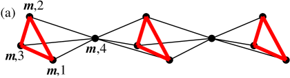
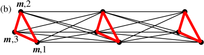
Figure 1: (Color online) Two 1D frustrated lattices with triangular trapping cells: (a) the double-tetrahedra chain and (b) the frustrated (cylindrical) three-leg ladder (or frustrated triangular tube). The exchange or hopping integrals along the equilateral triangles are $J_{2}>0$ or $t_{2}>0$ (bold bonds) whereas all other exchange or hopping integrals are $J_{1}>0$ or $t_{1}>0$ (thin bonds).

On these 1D lattices we consider the spin-1/2 Heisenberg antiferromagnet with the Hamiltonian

$$H_{\rm{s}}=\sum_{(ij)}J_{ij}{\bf{s}}_{i}\cdot{\bf{s}}_{j}-hS^{z},\;\;\;S^{z}=\sum_{i}s_{i}^{z}$$ (2.1)

and the repulsive Hubbard model

$$H_{\rm{e}}=\sum_{\sigma=\uparrow,\downarrow}H_{0,\sigma}+U\sum_{i}n_{i,\uparrow}n_{i,\downarrow},\;\;\;U>0,$$

$$H_{0,\sigma}=\sum_{(ij)}t_{ij}\left(c_{i,\sigma}^{\dagger}c_{j,\sigma}+c_{j,\sigma}^{\dagger}c_{i,\sigma}\right)+\mu\sum_{i}n_{i,\sigma}.$$ (2.2)

We use standard notations in Eqs. (2.1) and (II) and imply periodic boundary conditions. The exchange or hopping integrals acquire two values: $J_{2}>0$ or $t_{2}>0$ along the equilateral triangles (bold bonds in Fig. 1) and $J_{1}>0$ or $t_{1}>0$ along all other bonds (thin bonds in Fig. 1). It is convenient to label the lattice sites by a pair of indeces, where the first number enumerates the cells ($m=1,\ldots,{\cal{N}}$, ${\cal{N}}=N/4$ for the double-tetrahedra chain, ${\cal{N}}=N/3$ for the frustrated triangular tube, $N$ is the number of sites) and the second one enumerates the position of the site within the cell, see Fig. 1.

The one-particle (one-magnon or one-electron) energy spectra for both models (with $h=0$ or $\mu=0$) can easily be calculated yielding

$$\varepsilon_{1,2}(\kappa)=-\frac{3}{2}J_{2}-J_{1}=-\varepsilon,$$

$$\varepsilon_{3,4}(\kappa)=-2J_{1}\mp J_{1}\sqrt{1+\frac{3}{2}(1+\cos\kappa)}$$ (2.3)

(double-tetrahedra chain) and

$$\varepsilon_{1,2}(\kappa)=-\frac{3}{2}J_{2}-3J_{1}=-\varepsilon,$$

$$\varepsilon_{3}(\kappa)=-3J_{1}+3J_{1}\cos\kappa$$ (2.4)

(frustrated triangular tube) for the spin model and

$$\varepsilon_{1,2}(\kappa)=-t_{2}=-\varepsilon,$$

$$\varepsilon_{3,4}(\kappa)=t_{2}\mp\sqrt{t_{2}^{2}+6t_{1}^{2}(1+\cos\kappa)}$$ (2.5)

(double-tetrahedra chain) and

$$\varepsilon_{1,2}(\kappa)=-t_{2}=-\varepsilon,$$

$$\varepsilon_{3}(\kappa)=2t_{2}+6t_{1}\cos\kappa$$ (2.6)

(frustrated triangular tube) for the electron model. The flat (dispersionless) bands $\varepsilon_{1,2}(\kappa)=-\varepsilon$ allow to construct such wave packets of Bloch states which are localized on the triangles. These localized one-particle states read

$$|+\rangle_{m}=\frac{1}{\sqrt{3}}\left(s_{m,1}^{-}+\omega s_{m,2}^{-}+\omega^{2}s_{m,3}^{-}\right)|{\rm{FM}}\rangle,$$

$$|-\rangle_{m}=\frac{1}{\sqrt{3}}\left(s_{m,1}^{-}+\omega^{2}s_{m,2}^{-}+\omega s_{m,3}^{-}\right)|{\rm{FM}}\rangle,$$ (2.7)

where $|{\rm{FM}}\rangle$ denotes the ferromagnetic background for the spin model and

$$|+\rangle_{m}=\frac{1}{\sqrt{3}}\left(c_{m,1}^{\dagger}+\omega c_{m,2}^{\dagger}+\omega^{2}c_{m,3}^{\dagger}\right)|{\rm{0}}\rangle,$$

$$|-\rangle_{m}=\frac{1}{\sqrt{3}}\left(c_{m,1}^{\dagger}+\omega^{2}c_{m,2}^{\dagger}+\omega c_{m,3}^{\dagger}\right)|{\rm{0}}\rangle,$$ (2.8)

where $|{\rm{0}}\rangle$ denotes the vacuum state for the electron model and the spin index $\sigma$ is omitted as irrelevant for the one-electron problem. Here $\omega=e^{2\pi i/3}$.

The two-fold degeneracy of the flat bands corresponds to two possible values of the chirality of the triangle. For the spin model, after introducing the chirality operator for a trianglechirality-parameter

$$\chi_{m}=\frac{4}{\sqrt{3}}\left({\bf{s}}_{m,1}\cdot\left[{\bf{s}}_{m,2}\times{\bf{s}}_{m,3}\right]\right)$$

$$=\frac{2i}{\sqrt{3}}\left[\left(s_{m,1}^{+}s_{m,2}^{-}-s_{m,1}^{-}s_{m,2}^{+}\right)s_{m,3}^{z}\right.$$

$$\left.+\left(s_{m,2}^{+}s_{m,3}^{-}-s_{m,2}^{-}s_{m,3}^{+}\right)s_{m,1}^{z}\right.$$

$$\left.+\left(s_{m,3}^{+}s_{m,1}^{-}-s_{m,3}^{-}s_{m,1}^{+}\right)s_{m,2}^{z}\right],$$ (2.9)

we find $\chi_{m}|\pm\rangle_{m}=\pm|\pm\rangle_{m}$. We notice that the $s^{z}$ operators in Eq. (II) yield simply 1/2 after acting of $\chi_{m}$ on the states $|\pm\rangle_{m}$ (2.7). Therefore we may choose a simpler form of the chirality operator omitting the operators $s^{z}$ and the factor 2 in the last expression in Eq. (II), see, e.g., Ref. chirality-parameter, . Similarly, for the electron models

$$\chi_{m}=-\frac{i}{\sqrt{3}}\left(c_{m,1}^{\dagger}c_{m,2}+c_{m,1}c_{m,2}^{\dagger}\right.$$

$$\left.+c_{m,2}^{\dagger}c_{m,3}+c_{m,2}c_{m,3}^{\dagger}+c_{m,3}^{\dagger}c_{m,1}+c_{m,3}c_{m,1}^{\dagger}\right)$$ (2.10)

and again $\chi_{m}|\pm\rangle_{m}=\pm|\pm\rangle_{m}$. In both spin and electron cases the chirality operator $\chi_{m}$ can be written in the form

$$\chi_{m}=|+\rangle_{m}\langle+|_{m}-|-\rangle_{m}\langle-|_{m},$$ (2.11)

see Eqs. (2.7) and (2.8).

From the above equations for the spectra it is obvious that the two-fold degenerate flat band becomes the lowest one if $J_{2}>2J_{1}$ for the spin model or $t_{2}>2t_{1}$ for the electron model. In what follows we assume that these ratios are fulfilled.

III The contribution of independent localized states to thermodynamic quantities

The spin Hamiltonian (2.1) commutes with $S^{z}$, i.e., the number of magnons $n=N/2-S^{z}$ is a good quantum number. Similarly, the electron Hamiltonian (II) commutes with the operator of the number of electrons. Therefore, we may consider the subspaces with different numbers of magnons or electrons separately. Moreover, we may assume at first $h=0$ or $\mu=0$ and add trivial contributions of these terms to the partition function later.

We start with the construction of localized many-particle eigenstates in the subspaces with $n\leq n_{\max}\propto N$ magnons or electrons based on the localized one-particle states. These localized many-particle states are obtained by occupying the triangular traps with localized particles. For the occupation of the traps certain rules have to be fulfilled, cf. Ref. localized_magnons_b, for spin systems and Ref. localized_electrons, for electron systems. For the spin system on the frustrated-tube lattice localized magnons cannot occupy neighboring triangular traps whereas for the double-tetrahedra spin chain the occupation of neighboring triangular traps is allowed. Hence, according to Ref. localized_magnons_b, , the frustrated triangular spin tube belongs to the hard-dimer class and the double-tetrahedra spin chain belongs to the hard-monomer class. For both electron models localized electrons may occupy neighboring traps. Moreover, for the electron system it is possible that two electrons forming a spin-1 triplet (e.g., two spin-up electrons) but having different chiralities occupy the same triangular trap. Note that the different trap occupation rules lead finally to the different relations between the maximum number of localized magnons (electrons) $n_{\max}$ and the number of cells $\cal N$ given below.

It is helpful to bear in mind a simple picture visualizing this construction of the many-particle states.localized_magnons_a ; localized_magnons_b ; localized_electrons Namely, the construction of the many-particle states may be associated with a filling of an auxiliary lattice (a simple chain of ${\cal{N}}$ sites in all cases considered here) by hard-core objects (hard monomers or hard dimers) of two colors corresponding to two values of the chirality. Moreover, for the electron systems we have to take into account in addition the electron spin and the Pauli principle. Thus, the maximum filling with magnons is $n_{\max}={\cal{N}}$ (double-tetrahedra Heisenberg chain) and $n_{\max}={\cal{N}}/2$ (frustrated Heisenberg triangular tube), whereas for the Hubbard model the maximum filling with electrons is $n_{\max}=2{\cal{N}}$ for both lattices.

According to these rules the localized many-particle states are product states of localized one-particle states with the energy $E_{\rm{FM}}-n\varepsilon$ ($E_{\rm{FM}}$ is the energy of the ferromagnetic state) for the spin models or with the energy $-n\varepsilon$ for the electron models, where $\varepsilon$ is given in Eqs. (2.3) – (2.6). Importantly, localized electron eigenstates constructed in this way do not feel the Hubbard interaction $U$. Furthermore, the localized many-particle states are the only ground states in the corresponding subspaces with up to $n_{\max}$ magnons or electrons if $J_{2}>2J_{1}$ (spin models) or $t_{2}>2t_{1}$ (electron models). We have checked this analyzing full diagonalization data for several finite spin and electron systems. Obviously, there is a large manifold of degenerate localized many-particle ground states in an $n$-particle subspace. We will denote this ground-state degeneracy in what follows as $g_{\cal{N}}(n)$.

For the spin models the contribution of these localized eigenstates to the partition function is given by

$$Z_{{\rm{lm}}}(T,h,N)=\sum_{n=0}^{n_{\max}}g_{{\cal{N}}}(n)e^{-\frac{E_{{\rm{FM}}}-\frac{N}{2}h-n(h_{1}-h)}{T}}$$

$$=e^{-\frac{E_{{\rm{FM}}}-\frac{N}{2}h}{T}}\sum_{n=0}^{n_{\max}}g_{{\cal{N}}}(n)z^{n},\;\;\;z=e^{\frac{h_{1}-h}{T}},\;\;\;h_{1}=\varepsilon,$$ (3.1)

where the quantity $g_{{\cal{N}}}(n)$ represents the degeneracy of the ground-state manifold of $n$ magnons in a system with $\cal{N}$ traps. For the spin models it is easy to obtain (see Ref. localized_magnons_b, )

$$g_{{\cal{N}}}(n)=2^{n}{\cal{C}}_{\cal{N}}^{n}\;,\;{\cal{C}}_{\cal{N}}^{n}=\frac{{\cal{N}}!}{n!({\cal{N}}-n)!}$$ (3.2)

(double-tetrahedra chain) and

$$g_{{\cal{N}}}(n)=2^{n}{\cal{Z}}_{{\rm{hd}}}(n,{\cal{N}})$$ (3.3)

(frustrated triangular tube), where ${\cal{Z}}_{{\rm{hd}}}(n,{\cal{N}})$ is the canonical partition function of $n$ hard dimers on a periodic chain of ${\cal{N}}$ sites. The factor $2^{n}$ in the above expressions stems from the extra degeneracy due to the chirality degrees of freedom. After substitution of $g_{\cal{N}}(n)$ from Eq. (3.2) or Eq. (3.3) into Eq. (III) one obtains the free energy

$$\frac{F_{{\rm{lm}}}(T,h,N)}{{\cal{N}}}=\frac{E_{{\rm{FM}}}}{{\cal{N}}}-\frac{N}{2{\cal{N}}}h-T\ln\left(1+2z\right)$$ (3.4)

(double-tetrahedra chain) or

$$\frac{F_{{\rm{lm}}}(T,h,N)}{{\cal{N}}}=\frac{E_{{\rm{FM}}}}{{\cal{N}}}-\frac{N}{2{\cal{N}}}h-T\frac{\ln\left(\lambda_{1}^{{\cal{N}}}+\lambda_{2}^{{\cal{N}}}\right)}{{\cal{N}}},$$

$$\lambda_{1,2}=\frac{1}{2}\pm\sqrt{\frac{1}{4}+2z}\qquad\qquad\qquad$$ (3.5)

(frustrated triangular tube). At low temperatures and for magnetic fields $h$ around the saturation field $h_{1}=\varepsilon$ the contribution of localized states is dominating. Hence, $F_{{\rm{lm}}}(T,h,N)$ given in Eqs. (3.4) and (III) yields a good description of the low-temperature physics near the saturation field of the full spin model.

Analogously, the contribution of the localized eigenstates to the grand-canonical partition function of the electron models is given by

$$\Xi_{{\rm{le}}}(T,\mu,N)=\sum_{n=0}^{n_{\max}}g_{{\cal{N}}}(n)e^{-\frac{(-\varepsilon+\mu)n}{T}}$$

$$=\sum_{n=0}^{n_{\max}}g_{{\cal{N}}}(n)z^{n},\;\;\;z=e^{\frac{\varepsilon-\mu}{T}}.$$ (3.6)

To avoid the calculation of $g_{{\cal{N}}}(n)$ one may rewrite Eq. (III) as a sum over occupation numbers of each cell taking into account (i) that the cells are independent and (ii) that each cell may contain 0, 1, or 2 electrons having the degeneracy of the ground states $g_{1}(0)=1$, $g_{1}(1)=4$, or $g_{1}(2)=3$, respectively, see Ref. localized_electrons, . Thus, we have

$$\Xi_{{\rm{le}}}(T,\mu,N)=$$

$$\quad\sum_{n_{1}=0,1,2}\ldots\sum_{n_{\cal{N}}=0,1,2}g_{1}(n_{1})\ldots g_{1}(n_{{\cal{N}}})z^{n_{1}+\ldots+n_{{\cal{N}}}}$$

$$\qquad=\left[\sum_{n=0,1,2}g_{1}(n)z^{n}\right]^{\cal{N}}=\left(1+4z+3z^{2}\right)^{\cal{N}}$$ (3.7)

for both lattices, the double-tetrahedra chain and the frustrated triangular tube. Eq. (III) immediately yields the required grand-thermodynamical potential

$$\frac{\Omega_{{\rm{le}}}(T,\mu,N)}{{\cal{N}}}=-T\ln\left(1+4z+3z^{2}\right).$$ (3.8)

Again, at low temperatures and for chemical potentials $\mu$ around $\mu_{0}=\varepsilon$ the contribution of localized states is dominating, and $\Omega_{{\rm{le}}}(T,\mu,N)$ given in Eq. (3.8) yields a good description of the low-temperature physics of the full electron model.

We mention that the obtained formulas for the free energy and the grand-thermodynamical potential are similar (but not identical) to those derived in previous papers,localized_magnons_b ; localized_electrons the deviations from the previously derived equations are related to the chirality degrees of freedom.

Let us briefly discuss the low-temperature thermodynamics as it follows from Eqs. (3.4), (III), and (3.8). The main low-temperature features of the spin models for $h$ around $h_{1}$ are as follows: (i) a jump in the ground-state magnetization curve at the saturation field $h_{1}$ with a preceding wide plateau, (ii) a nonzero residual ground-state entropy at the saturation field $h_{1}$, (iii) a low-temperature peak in the specific heat, which moves to $T=0$ as $h$ approaches $h_{1}$. Correspondingly, for the electron models we have: (i) a zero-temperature jump in the averaged number of electrons as a function of the chemical potential at $\mu=\mu_{0}$, (ii) a nonzero residual ground-state entropy for $\mu=\mu_{0}$ (or as a function of the electron concentration $c=n/{\cal{N}}$ for $c\leq 2$), (iii) a low-temperature peak in the grand-canonical specific heat $C(T,\mu,N)$, but a vanishing low-temperature canonical specific heat $C(T,n,N)=0$ for $n\leq n_{\max}$ (see also the discussion in Ref. dj, ).

The temperature dependence of the specific heat of the spin models is shown in Fig. 2. By comparison of the hard-core data obtained from Eqs. (3.4), (III) with exact-diagonalization data of the full spin model we can estimate the range of validity of the hard-core description. The low-temperature parts of the curves for the specific heat obtained from exact diagonalization (symbols) and from the hard-core description (dashed lines) coincide at least up to $T=0.15$. For both Heisenberg chains the specific heat shows in addition to the typical high-temperature maximum around $T\sim J_{2}$ a low-temperature maximum which is well described by the hard-core models. This low-temperature maximum can be ascribed to an extra low-energy scale set by the localized eigenstates. Interestingly, for the frustrated triangular tube there is even a third maximum which can be related to a third energy scale set by another class of highly degenerate eigenstates, the so-called interacting localized-magnon states, which will be discussed in the next section.

There are no finite-size effects in the hard-monomer description (3.4). To illustrate the finite-size dependence inherent in the hard-dimer description (III), we compare in panels (c) and (d) of Fig. 2 results for finite $\cal N$ (dashed lines) with data for ${\cal{N}}\to\infty$ (thin dashed lines). Clearly, finite-size effects are obvious only at low temperatures for $h$ below the saturation field $h_{1}$.

The high degeneracy of the localized eigenstates leads to a residual ground-state entropy given by $S(T=0,h=h_{1},N)/{\cal{N}}=\ln 3\approx 1.099$ (double-tetrahedra spin chain) and $S(T=0,h=h_{1},N)/{\cal{N}}=\ln 2\approx 0.693$ (frustrated triangular spin tube). Due to the chirality these numbers exceed the corresponding results reported in Ref. localized_magnons_b, b for the standard diamond spin chain $S(T=0,h=h_{1},N)/{\cal{N}}=\ln 2\approx 0.693$ and the frustrated two-leg spin ladder $S(T=0,h=h_{1},N)/{\cal{N}}=\ln[(1+\sqrt{5})/2]\approx 0.481$.

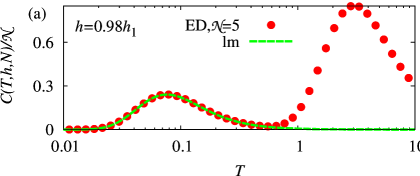
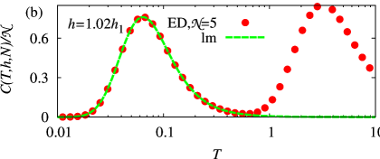
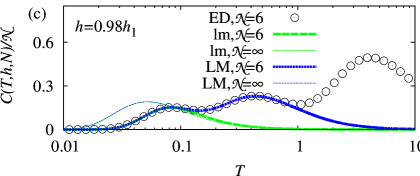
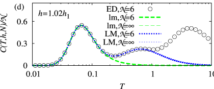
Figure 2: (Color online) Specific heat $C(T,h,N)/{\cal{N}}$ vs temperature $T$ for $h$ around $h_{1}$ for [(a) and (b)] the $N=20$ double-tetrahedra spin chain and [(c) and (d)] the $N=18$ frustrated triangular spin tube. $J_{1}=1$, $J_{2}=5$; symbols correspond to exact-diagonalization data, dashed lines correspond to independent localized-magnon predictions derived from Eqs. (3.4) and (III) (abbreviation lm), dotted lines correspond to interacting localized-magnon predictions derived form Eq. (IV) (abbreviation LM, for the frustrated triangular tube only). The thin dashed and thin dotted lines in panels (c) and (d) correspond to localized-magnon predictions in the limit ${\cal{N}}\to\infty$. Note that some curves in panels (c) and (d) practically coincide. Namely in panel (c), thin dashed and thin dotted lines are indistinguishable at low temperatures, whereas at higher temperatures dashed and thin dashed (dotted and thin dotted) lines coincide. In panel (d) dashed and thin dashed (dotted and thin dotted) lines cannot be distinguished.

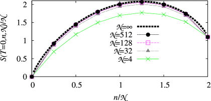
Figure 3: (Color online) Residual ground-state entropy $S(T=0,n,{\cal{N}})/{\cal{N}}$ vs electron concentration $c=n/{\cal{N}}$ for the Hubbard model with $t_{2}>2t_{1}$ on the double-tetrahedra chain and the frustrated triangular tube (the data for both systems are identical). Note that the curves becomes indistinguishable in the scale of the figure as ${\cal{N}}$ increases.

For the Hubbard model we have calculated curves for the grand-canonical specific heat similar to those for the Heisenberg model, which for the sake of brevity are not shown here. They also exhibit an additional low-temperature maximum for $\mu\lesssim\mu_{0}$ and $\mu\gtrsim\mu_{0}$ which is well described by the localized eigenstates, see also Ref. localized_electrons, . The residual ground-state entropy $\lim_{T\to 0}S(T,n,N)=\ln g_{{\cal{N}}}(n)$ as a function of the electron concentration $c=n/{\cal{N}}$ for the Hubbard model is shown in Fig. 3. According to Eq. (III) for finite systems one has $n!g_{\cal{N}}(n)={d^{n}\Xi_{{\rm{le}}}(z,N)/dz^{n}}|_{z=0}$. Using Eq. (III) one obtains $g_{{\cal{N}}}(n)$ for (small) finite ${\cal{N}}$. For ${\cal{N}}=4$ the analytical predictions which follow from Eqs. (III), (3.8) coincide with exact-diagonalization data for the full Hubbard model, e.g., $g_{4}(n)=1,16,108,400,886,1200,972,432,81$ for $n=0,1,2,3,4,5,6,7,8$. Using Eq. (3.8) by means of standard relations of statistical mechanics we find for the residual ground-state entropy in the thermodynamic limit $S(T=0,n,N)/{\cal{N}}=\ln(1+4z+3z^{2})-(4z\ln z+6z^{2}\ln z)/(1+4z+3z^{2})$ with $z=[2(1-c)-\sqrt{c^{2}-2c+4}]/[3(c-2)]$, $c=n/{\cal{N}}$, see the dotted curve in Fig. 3. This quantity reaches its maximum, $3\ln 2\approx 2.079$, at $c=n/{\cal{N}}=5/4$. Moreover, it equals $\ln 3\approx 1.099$ at $c=n/{\cal{N}}=2$. Obviously, the chirality leads to an increase of the residual ground-state entropy. While for the Hubbard model on the diamond chain and the frustrated two-leg ladder $S(T=0,\mu=\mu_{0},N)/{\cal{N}}=\ln 3\approx 1.099$ (see Ref. localized_electrons, b), for the considered lattices $S(T=0,\mu=\mu_{0},N)/{\cal{N}}=3\ln 2\approx 2.079$.

IV Beyond independent localized magnons

For the frustrated-tube spin model we can extend the hard-dimer description taking into account additional low-energy states following the lines described in Ref. labi, . If one allows the occupation of neighboring traps by localized magnons (i.e., relaxing the hard-dimer rule) one has also an eigenstate of the spin Hamiltonian, however with a higher energy. More precisely, if two localized magnons become neighbors the energy increases by $J_{1}$. Importantly, these localized-magnon states are also highly degenerate and they are the lowest excitations above the independent localized-magnon ground states for $S^{z}=N/2,\ldots,N/2-{\cal{N}}/2$ if $J_{2}>J_{2}^{c}$ (strong-coupling regime). Based on finite-size calculations for $N=18,\dots,72$ we estimate $J_{2}^{c}/J_{1}\approx 2.68>2$. These additional eigenstates can be described as interacting localized-magnon states, where the repulsive interaction $V=J_{1}$ is responsible for the energy increase with respect to the independent localized-magnon states. Taking into account this finite repulsion $V$ in the partition function of the lattice-gas model with nearest-neighbor interaction we have then [instead of Eq. (III)]

$$Z_{{\rm{LM}}}(T,h,N)=e^{-\frac{E_{{\rm{FM}}}-\frac{N}{2}h}{T}}\sum_{n_{1}=0,1}\ldots\sum_{n_{{\cal{N}}}=0,1}g_{1}(n_{1})$$

$$\times\ldots g_{1}(n_{\cal{N}})z^{n_{1}+\ldots+n_{\cal{N}}}e^{-\frac{V(n_{1}n_{2}+n_{2}n_{3}+\ldots+n_{\cal{N}}n_{1})}{T}}\quad$$ (4.1)

with $g_{1}(0)=1$, $g_{1}(1)=2$ and $z$ is defined in Eq. (III). In Eq. (IV) we have used a representation in terms of the cell occupation numbers $n_{i}$, cf. Eq. (III). Obviously, Eq. (III) is obtained from Eq. (IV) for $V\to\infty$. Evaluating the sums in Eq. (IV) by means of the transfer-matrix method we arrive at the following result for the free energy

$$\frac{F_{{\rm{LM}}}(T,h,N)}{{\cal{N}}}=\frac{E_{{\rm{FM}}}}{\cal{N}}-\frac{N}{2{\cal{N}}}h-T\frac{\ln\left(\lambda_{1}^{\cal{N}}+\lambda_{2}^{\cal{N}}\right)}{\cal{N}},$$

$$\lambda_{1,2}=\frac{1}{2}+ze^{-\frac{V}{T}}\pm\sqrt{\frac{1}{4}+2z-ze^{-\frac{V}{T}}+z^{2}e^{-\frac{2V}{T}}}.$$ (4.2)

Note that the lattice-gas model with finite repulsion (IV), (IV) takes into account $3^{{\cal{N}}}\approx 1.442^{N}$ statesfootnote1 of the $2^{N}$ eigenstates of the initial quantum spin model (2.1), whereas hard-dimer model (III), (3.3), (III) has only $2^{{\cal{N}}}\approx 1.260^{N}$ states.footnote2 On the other hand, the hard-monomer model (III), (3.2), (3.4) has $3^{{\cal{N}}}\approx 1.316^{N}$ states.footnote1

The specific heat derived from Eq. (IV) is plotted in Fig. 2, panels (c) and (d), dotted and thin dotted lines. Indeed, the inclusion of the interacting localized-magnon states leads to a significant improvement of the lattice-gas description. The lattice-gas model with finite repulsion (IV), (IV) covers the thermodynamics of the full spin model at least up to $T=0.9$ for $h\sim h_{1}$ including the two maxima below the typical high-temperature maximum around $T\sim J_{2}$. Again finite-size effects are more important at low temperatures for $h$ below the saturation field $h_{1}$, see thin dotted lines in panels (c) and (d) of Fig. 2.

The interacting localized-magnon states being excitations for $S^{z}=N/2,\ldots,N/2-{\cal{N}}/2$ can become ground states for smaller values of $S^{z}$. The ground-state magnetization curve $\langle M\rangle=2S^{z}/N$ vs $h$ for the frustrated triangular spin tube presented in Ref. andreas, exhibits two plateaus at $\langle M\rangle=2/3$ for $h_{2}<h<h_{1}$ and at $\langle M\rangle=1/3$ for $h_{3}<h<h_{2}$ and two jumps at $h=h_{1}$ and $h=h_{2}$, where $h_{1}=3J_{1}+3J_{2}/2$, $h_{2}=J_{1}+3J_{2}/2$, and $h_{3}=2J_{1}$. In the language of localized magnons the $2/3$-plateau corresponds to the maximum filling with $n=n_{\max}={\cal N}/2$ independent localized magnons (i.e., every second trap is occupied and $S^{z}=N/2-{\cal N}/2=N/3$). If $n_{\max}<n\leq 2n_{\max}$ (i.e., $N/2-{\cal{N}}\leq S^{z}<N/2-{\cal{N}}/2$), the ground states in the strong-coupling regime are obtained by filling the remaining empty cells (i.e., the hard-dimer rule is relaxed) thus having interacting localized-magnon states as ground states. Then the very broad $1/3$-plateau corresponds to the complete filling of all cells with $n=2n_{\max}={\cal N}$ localized magnons. Hence, with the improved effective theory given in Eq. (IV) we can provide an accurate description of the low-temperature physics of the frustrated triangular spin tube in the strong-coupling regime not only near the saturation field $h_{1}$ up to quite large temperatures as shown in Fig. 2, but also for much lower magnetic fields in the entire region of the $2/3$-plateau and even for fields within the $1/3$-plateau being not too far from $h_{2}$, see Fig. 4. It might be interesting to recall that the lattice-gas model with finite repulsion provides similar description of the frustrated two-leg spin ladder around both characteristic fields $h_{1}$ and $h_{2}$.labi This is not the case for the frustrated triangular spin tube because of the chirality degrees of freedom, compare the results for $h=10$ and $h=9$ in Fig. 4.

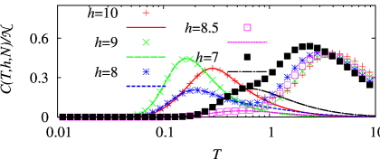
Figure 4: (Color online) Specific heat $C(T,h,N)/{\cal{N}}$ vs temperature $T$ for finite frustrated triangular spin tubes of $N=18$ sites (${\cal{N}}=6$ cells) with $J_{1}=1$, $J_{2}=5$ ($h_{1}=10.5$) for various magnetic fields down to values below $h_{2}=8.5$ (lines – lattice-gas model with finite repulsion, symbols – exact-diagonalization data for the full spin model).

V Lifting the degeneracy due to chirality degrees of freedom

As discussed above the chirality degrees of freedom lead to an extra degeneracy of the independent localized-magnon or localized-electron ground states in the subspace with $n\leq n_{\max}$ magnons or electrons. Moreover, the interacting localized-magnon states discussed for the frustrated triangular spin tube also carry this extra degree of freedom. This degeneracy of the eigenstates owing to the chirality may be lifted by a small symmetry-breaking perturbation. As a rule, perturbations of ideal model Hamiltonians may lead to a more realistic description of real systems. We consider here separately for the spin systems the case of a Zeeman-like perturbation (which corresponds to a Dzyaloshinskii-Moriya interaction between neighboring spins in a triangular trap), see Sec. V.1, and the case of an $XX$-like perturbation acting on (pseudo)spin variables representing chiralities (which corresponds to a four-site interaction between spin pairs in neighboring traps), see Sec. V.3. For the Hubbard model appropriate perturbations correspond to a magnetic field perpendicular to the triangular traps and a four-site electron-electron interaction, see Sec. V.2 and Sec. V.3.

V.1 Dzyaloshinskii-Moriya interaction

We consider the spin system in the subspaces with $n\leq n_{\max}$ magnons. The ground state has the energy $E_{\rm{FM}}-n\varepsilon$ ($h=0$) and the degeneracies $g_{\cal{N}}(n)$ are given in Eqs. (3.2) or (3.3). The factor $2^{n}$ present in these formulas for $g_{\cal{N}}(n)$ is due to the chirality of localized magnons. We introduce the (pseudo)spin-1/2 operators

$$\tau_{m}^{z}=\frac{1}{2}\left(|+\rangle_{m}\langle+|_{m}-|-\rangle_{m}\langle-|_{m}\right)=\frac{1}{2}\chi_{m},$$ (5.1)

where $\chi_{m}=(i/\sqrt{3})(s_{m,1}^{+}s_{m,2}^{-}-s_{m,1}^{-}s_{m,2}^{+}+s_{m,2}^{+}s_{m,3}^{-}-s_{m,2}^{-}s_{m,3}^{+}+s_{m,3}^{+}s_{m,1}^{-}-s_{m,3}^{-}s_{m,1}^{+})$ is the chirality operator, see Eq. (II) and the discussion below this equation. We now add to the spin Hamiltonian (2.1) a small perturbation

$$H_{\rm{s}}^{(1)} = \frac{i\epsilon^{(1)}}{2\sqrt{3}}\sum_{m}\left(s_{m,1}^{+}s_{m,2}^{-}-s_{m,1}^{-}s_{m,2}^{+}\right.$$

$$\left.+s_{m,2}^{+}s_{m,3}^{-}-s_{m,2}^{-}s_{m,3}^{+}+s_{m,3}^{+}s_{m,1}^{-}-s_{m,3}^{-}s_{m,1}^{+}\right)$$

$$= D\sum_{m}\left(s_{m,1}^{x}s_{m,2}^{y}-s_{m,1}^{y}s_{m,2}^{x}\right.$$

$$\left.+s_{m,2}^{x}s_{m,3}^{y}-s_{m,2}^{y}s_{m,3}^{x}+s_{m,3}^{x}s_{m,1}^{y}-s_{m,3}^{y}s_{m,1}^{x}\right),$$

where the last expression in Eq. (V.1) corresponds to a Dzyaloshinskii-Moriya interaction ${\vec{D}}=D{\vec{e}_{z}}$, $D=\epsilon^{(1)}/\sqrt{3}$ between neighboring spins within each triangular trap. Note that the perturbation $H_{\rm{s}}^{(1)}$ commutes with $S^{z}$. According to the discussion of the chirality operator (II) in Sec. II it is obvious that the localized states are also eigenstates of the perturbation Hamiltonian (V.1). The set of $2^{n}$ degenerate ground states in the unperturbed system belonging to one particular spatial configuration of $n$ magnons placed in a certain (allowed) set of traps now splits into $n+1$ subsets of levels. The subsets are characterized by the magnon numbers $n_{+}$ and $n_{-}$ ($n_{+}+n_{-}=n$), belonging to the chirality indeces $+$ and $-$, respectively. There are $n!/(n_{+}!n_{-}!)$ degenerate states in the subset with energy $E_{\rm{FM}}-n\varepsilon+(n_{+}-n_{-})\epsilon^{(1)}/2$. The effective Hamiltonian acting in the subspace of the $g_{\cal{N}}(n)$ former $n$-magnon ground states of the unperturbed system reads

$${\cal{H}}_{\rm{s}}+{\cal{H}}_{\rm{s}}^{(1)}=E_{\rm{FM}}-n\varepsilon+\epsilon^{(1)}\sum_{m}\tau_{m}^{z},$$ (5.3)

where the sum runs over the $n$ occupied traps only.

We consider now the partition function of the spin model with the Hamiltonian $H_{\rm{s}}+H_{\rm{s}}^{(1)}$, Eqs. (2.1) and (V.1), at low temperatures and $h$ close to $h_{1}$. The dominant contribution to the partition function of the spin system comes from the low-energy degrees of freedom, which are governed by the Hamiltonian (5.3). Therefore the partition function is given by Eq. (III) replacing $g_{\cal{N}}(n)$ by ${\tilde{g}}_{\cal{N}}(n)=\{2\cosh[\epsilon^{(1)}/(2T)]\}^{n}{\cal{C}}_{\cal{N}}^{n}$ (double-tetrahedra chain) and ${\tilde{g}}_{\cal{N}}(n)=\{2\cosh[\epsilon^{(1)}/(2T)]\}^{n}{\cal{Z}}_{\rm{hd}}(n,{\cal{N}})$ (frustrated triangular tube), cf. Eqs. (3.2) and (3.3). As a result, the free energy reads

$$\frac{F_{{\rm{lm}}}(T,h,N)}{{\cal{N}}}=\frac{E_{{\rm{FM}}}}{{\cal{N}}}-\frac{N}{2{\cal{N}}}h-T\ln\left(1+2\cosh\frac{\epsilon^{(1)}}{2T}z\right)$$ (5.4)

(double-tetrahedra chain) and

$$\frac{F_{{\rm{lm}}}(T,h,N)}{{\cal{N}}} = \frac{E_{{\rm{FM}}}}{{\cal{N}}}-\frac{N}{2{\cal{N}}}h-T\frac{\ln\left(\lambda_{1}^{{\cal{N}}}+\lambda_{2}^{{\cal{N}}}\right)}{{\cal{N}}},$$

$$\lambda_{1,2} = \frac{1}{2}\pm\sqrt{\frac{1}{4}+2\cosh\frac{\epsilon^{(1)}}{2T}z}$$ (5.5)

(frustrated triangular tube), cf. Eqs. (3.4) and (III). Similar to Sec. IV, we can take into account interacting localized-magnon states also for the perturbed frustrated triangular tube described by the Hamiltonian $H_{\rm{s}}+H_{\rm{s}}^{(1)}$. The improved free energy $F_{{\rm{LM}}}(T,h,N)$ is then given by Eq. (IV), where $2z$ has to be substituted by $2\cosh[\epsilon^{(1)}/(2T)]z$.

In Fig. 5 we compare exact-diagonalization data for perturbed spin systems with predictions based on Eq. (5.4) and improved Eq. (V.1). Small perturbations lead to splitting of the ground-state levels and therefore to arising of one more low-energy scale. As a result, low-temperature features close to $h_{1}$ are more subtle. Thus temperature profiles of the specific heat for the spin systems show more tiny features which can be seen in Fig. 5. For a special set of parameters the temperature dependence $C$ vs $T$ may exhibit even three (four) maxima for the double-tetrahedra chain (frustrated triangular tube). The low-temperature maxima are excellently described within the effective low-energy theory, see Fig. 5.

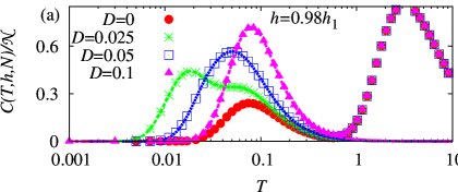
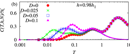
Figure 5: (Color online) Specific heat $C(T,h,N)/{\cal{N}}$ vs temperature $T$ for $h=0.98h_{1}$ for the spin model (2.1), (V.1) on (a) the double-tetrahedra chain and (b) the frustrated triangular tube. Exact-diagonalization data (symbols) versus analytical predictions (lines) according to Eq. (5.4) (double-tetrahedra chain) and improved Eq. (V.1) (frustrated triangular tube) for finite systems of ${\cal{N}}=4$ cells with $J_{1}=1$, $J_{2}=5$, and $D=0,\,0.025,\,0.05,\,0.1$.

V.2 Electrons in a magnetic field

In analogy to the above discussion for perturbed spin models, we consider the case of $n\leq n_{\max}$ Hubbard electrons (II) with a perturbation

$$H_{\rm{e}}^{(1)}=\sum_{\sigma=\uparrow,\downarrow}H_{0,\sigma}^{(1)},$$

$$H_{0,\sigma}^{(1)}=ig\sum_{m}\left(c_{m,1,\sigma}^{\dagger}c_{m,2,\sigma}+c_{m,1,\sigma}c_{m,2,\sigma}^{\dagger}\right.$$

$$\left.+c_{m,2,\sigma}^{\dagger}c_{m,3,\sigma}+c_{m,2,\sigma}c_{m,3,\sigma}^{\dagger}\right.$$

$$\left.+c_{m,3,\sigma}^{\dagger}c_{m,1,\sigma}+c_{m,3,\sigma}c_{m,1,\sigma}^{\dagger}\right),$$ (5.6)

where $ig$ is a pure imaginary component of the hopping integral between neighboring sites along the triangular traps. For the perturbed Hamiltonian the number of electrons remains a conserved quantity and the localized states are its eigenstates, cf. the chirality operator (II) in Sec. II. The perturbation considered here corresponds to a magnetic field perpendicular to the triangular trap. Then the hoping integral $t_{{\bf{i}}{\bf{j}}}$ acquires the Peierls phase factor $e^{(2i\pi/\Phi_{0})\int_{{\bf{i}}}^{{\bf{j}}}d{\bf{r}}\cdot{\bf{A}}}$, where $\Phi_{0}=hc/e$ is the flux quantum, ${\bf{A}}$ is the vector potential of the external magnetic field, see Refs. essler, ; gula, . The effective Hamiltonian acting in the subspace of the $g_{\cal{N}}(n)$ former $n$-electron ground states of the unperturbed system reads

$${\cal{H}}_{\rm{e}}+{\cal{H}}_{\rm{e}}^{(1)}=-n\varepsilon+\epsilon^{(1)}\sum_{m}\tau_{m}^{z},$$ (5.7)

where $\epsilon^{(1)}=-2\sqrt{3}g$ and the sum runs over the $n$ occupied traps only.

We consider now the grand-canonical partition function of the electron models with the Hamiltonian $H_{\rm{e}}+H_{\rm{e}}^{(1)}$, Eqs. (II) and (V.2), at low temperatures and $\mu$ close to $\mu_{0}=\varepsilon$. The dominant contribution to the grand-canonical partition function comes from the low-energy states, which are governed by the Hamiltonian (5.7). Repeating the arguments which lead to Eq. (3.8) we arrive now at

$$\frac{\Omega_{{\rm{le}}}(T,\mu,N)}{{\cal{N}}}=-T\ln\left(1+4\cosh\frac{\epsilon^{(1)}}{2T}z+3z^{2}\right),$$ (5.8)

where $z=e^{(\varepsilon-\mu)/T}$, cf. Eqs. (III) – (3.8).

We focus on the low-temperature behavior of the entropy of the perturbed electron model. We can easily find, using a simple counting of states, the residual ground-state entropy, namely, $S(T=0,n,{\cal{N}})=\ln\left(2^{n}{\cal{C}}_{\cal{N}}^{n}\right)$ for $n=0,\ldots,{\cal{N}}$ and $S(T=0,n,{\cal{N}})=\ln\left(3^{n-{\cal{N}}}2^{2{\cal{N}}-n}{\cal{C}}_{\cal{N}}^{n-{\cal{N}}}\right)$ for $n={\cal{N}},\ldots,2{\cal{N}}$. In the thermodynamic limit ${\cal{N}}\to\infty$ this gives: $S(T=0,n,{\cal{N}})/{\cal{N}}=c\ln 2-c\ln c-(1-c)\ln(1-c)$ for $0\leq c\leq 1$ and $S(T=0,n,{\cal{N}})/{\cal{N}}=(c-1)\ln 3+(2-c)\ln 2-(c-1)\ln(c-1)-(2-c)\ln(2-c)$ for $1\leq c\leq 2$, where $c=n/\cal{N}$. For the special electron concentrations $c=1$ and $c=2$ one has $S(T=0)/{\cal{N}}=\ln 2\approx 0.693$ and $S(T=0)/{\cal{N}}=\ln 3\approx 1.099$, respectively. For finite temperatures we find from Eq. (5.8) $S(T,n,{\cal{N}})/{\cal{N}}=\ln\{1+4\cosh[\epsilon^{(1)}/(2T)]z+3z^{2}\}-\{2(\epsilon^{(1)}/T)\sinh[\epsilon^{(1)}/(2T)]z+4\cosh[\epsilon^{(1)}/(2T)]z\ln z+6z^{2}\ln z\}/\{1+4\cosh[\epsilon^{(1)}/(2T)]z+3z^{2}\}$ with $z=\{2(1-c)\cosh[\epsilon^{(1)}/(2T)]-\sqrt{4(c-1)^{2}\cosh^{2}[\epsilon^{(1)}/(2T)]-3c(c-2)}\}/[3(c-2)]$.

In Fig. 6 we show the entropy $S(T,n,N)$ of the perturbed electron systems obtained by the above given formulas versus the electron concentration $c=n/\cal{N}$. To estimate the region of validity of these results we compared first exact-diagonalization data for the grand-canonical specific heat $C(T,\mu,N)$ for finite perturbed electron systems (e.g., for ${\cal{N}}=2$, $t_{1}=1$, $t_{2}=3$ and $t_{2}=5$, $g=0.1$, $\mu=0.98\mu_{0},\,\mu_{0},\,1.02\mu_{0}$) with analytical results for $C(T,\mu,N)$ based on Eq. (5.8). (For the sake of brevity we do not show these results explicitely.) We find an excellent agreement between these results at least up to $T=0.2$ for $t_{2}=3$ (and even for higher temperatures for larger values of $t_{2}$). For nonzero but low temperatures (e.g., $T=0.15$) $S(T,n,{\cal{N}})/{\cal{N}}$ behaves as in Fig. 3, see panel (c) of Fig. 6. However, at lower temperatures (e.g., $T=0.075$ and $T=0.015$) the smallest energy scale comes into play, and the entropy changes remaining nonzero in the ground state, see panels (b) and (a) of Fig. 6. In spite of the partial degeneracy lifting due to the perturbation (V.2), the ground states remain hugely degenerate and exhibit a nonzero residual ground-state entropy for electron concentrations $0<c=n/{\cal{N}}\leq 2$, see panel (a) of Fig. 6 ($T=0.015$).

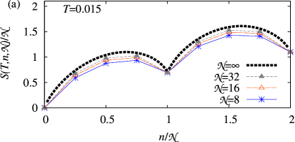
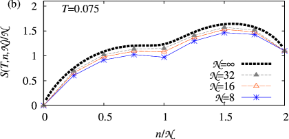
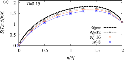
Figure 6: (Color online) Entropy $S(T,n,{\cal{N}})/{\cal{N}}$ vs electron concentration $c=n/{\cal{N}}$ at low temperatures (a) $T=0.015$, (b) $T=0.075$, and (c) $T=0.15$ for the Hubbard model (II) with $t_{2}>2t_{1}$ completed by small perturbation (V.2) with $g=0.1$ on the double-tetrahedra chain and the frustrated triangular tube. Analytical predictions are obtained according to Eq. (5.8) for systems of ${\cal{N}}=8,\;16,\;32$, and ${\cal{N}}\to\infty$ cells.

V.3 Interacting pseudospins

Now we consider the double-tetrahedra spin chain at the $\langle M\rangle=1/2$ plateau (i.e., there are $n=n_{\max}=\cal{N}$ magnons in the spin system, that is the so-called localized-magnon crystal state). We add a perturbation which can be understood as an $XX$ interaction of chirality pseudospins on neighboring trapping cells. The (pseudo)spin raising and lowering operators are defined as

$$\tau_{m}^{+}=|+\rangle_{m}\langle-|_{m},\;\;\;\tau_{m}^{-}=|-\rangle_{m}\langle+|_{m}.$$ (5.9)

They can be expressed by bilinear forms in the spin operators $s^{-}$ and $s^{+}$ attached to the $m$th cell, see Eq. (2.7). Clearly, $\tau_{m}^{+}|+\rangle_{m}=0$, $\tau_{m}^{+}|-\rangle_{m}=|+\rangle_{m}$, $\tau_{m}^{-}|+\rangle_{m}=|-\rangle_{m}$, $\tau_{m}^{-}|-\rangle_{m}=0$. The perturbation added to the Hamiltonian (2.1) reads

$$H_{\rm{s}}^{(2)}=\frac{\epsilon^{(2)}}{9}\sum_{m}\left[\left(s_{m,1}^{-}+\omega s_{m,2}^{-}+\omega^{2}s_{m,3}^{-}\right)\right.$$

$$\left.\times\left(s_{m,1}^{+}+\omega s_{m,2}^{+}+\omega^{2}s_{m,3}^{+}\right)\right.$$

$$\left.\times\left(s_{m+1,1}^{-}+\omega^{2}s_{m+1,2}^{-}+\omega s_{m+1,3}^{-}\right)\right.$$

$$\left.\times\left(s_{m+1,1}^{+}+\omega^{2}s_{m+1,2}^{+}+\omega s_{m+1,3}^{+}\right)+{\rm{H.c.}}\right],$$ (5.10)

where the sum runs over all trapping cells and $\omega=e^{2\pi i/3}$. Obviously, that corresponds to certain four-site interactions with the interaction constant $\epsilon^{(2)}/9$. The perturbation Hamiltonian $H_{\rm{s}}^{(2)}$ commutes with $S^{z}$. Moreover, after acting on the localized-magnon crystal state the perturbation Hamiltonian $H_{\rm{s}}^{(2)}$ changes the chirality indeces only. The effective Hamiltonian acting in the subspace of the localized-magnon crystal states of the unperturbed system now reads

$${\cal{H}}_{\rm{s}}+{\cal{H}}_{\rm{s}}^{(2)}=E_{\rm{FM}}-n\varepsilon+\epsilon^{(2)}\sum_{m=1}^{{\cal{N}}}\left(\tau_{m}^{+}\tau_{m+1}^{-}+{\rm{H.c.}}\right).$$ (5.11)

Due to the perturbation ${\cal{H}}_{\rm{s}}^{(2)}$ the $2^{{\cal{N}}}$-fold degenerate ground state of the double-tetrahedra spin chain with $n=n_{\max}={\cal{N}}$ magnons splits into ${\cal{N}}+1$ groups of sublevels. Moreover, the effective (pseudo)spin-1/2 $XX$ chain (5.11) is the exactly solvable modellieb and therefore we immediately obtain for the partition function $Z(T,n,N)$, $n=N/2-S^{z}$ of the double-tetrahedra spin chain with a Hamiltonian given by the sum of the terms in Eqs. (2.1) and (V.3) the following dominant contribution at low temperatures for the magnetization $S^{z}=N/2-n_{\max}=N/4$

$$Z_{{\rm{lm}}}(T,n_{\max},N)=e^{-\frac{E_{\rm{FM}}-{\cal{N}}\varepsilon}{T}}\prod_{\kappa}2\cosh\frac{\epsilon^{(2)}\cos\kappa}{T},$$ (5.12)

$\kappa=2\pi l/{\cal{N}}$, $l=-{\cal{N}}/2,-{\cal{N}}/2+1,\ldots,{\cal{N}}/2-1$ (we assume without loss of generality that ${\cal{N}}$ is even). Low-temperature thermodynamic quantities in the thermodynamic limit ${\cal{N}}\to\infty$ follow from the free energy

$$\frac{F_{{\rm{lm}}}\left(T,n_{\max},N\right)}{\cal{N}}=\frac{E_{\rm{FM}}}{{\cal{N}}}-\varepsilon$$

$$-\frac{T}{2\pi}\int_{-\pi}^{\pi}d\kappa\ln\left(2\cosh\frac{\epsilon^{(2)}\cos\kappa}{T}\right).$$ (5.13)

Note that the perturbation (V.1) can also be included. Then the formula (V.3) has to be slightly modified, namely, $2\epsilon^{(2)}\cos\kappa$ in Eq. (V.3) has to be replaced by $\epsilon^{(1)}+2\epsilon^{(2)}\cos\kappa$. Thus, including both perturbations (V.1) and (V.3) we arrive at an effective (pseudo)spin-1/2 $XX$ chain in a transverse field which governs the low-temperature physics of the double-tetrahedra chain in the subspace with $n=n_{\max}={\cal{N}}$ magnons (i.e., at the magnetization $S^{z}=N/2-n_{\max}=N/4$). It might be interesting to mention here that the spin-1/2 $XX$ chain in a transverse field also emerges as an effective low-energy model for the diamond spin chain at high magnetic fields if the conditions ensuring the presence of localized magnons become slightly violated.effective_xy For such a generalized diamond chain the spin-1/2 transverse $XX$ chain describes a weak spreading of the independent localized magnons over the whole chain. Another related model, the so-called spin-chirality model, is used for effective description of three-leg spin tubes within the perturbation theory approach from the strong rung-coupling limit, see Ref. sakai, and references therein. We stress here that in the case at hand the spin-1/2 transverse $XX$ chain describes propagating of chirality over the whole chain in the localized-magnon crystal state.

We consider next the frustrated triangular tube again in the subspace with $n=n_{\max}={\cal{N}}/2$ magnons (i.e., at the $\langle M\rangle=2/3$ plateau). The ground state, besides the degeneracy owing to chirality, is two-fold degenerate, i.e., the independent localized magnons may occupy either even-site or odd-site sublattice only. The perturbation to lift the degeneracy of the localized-magnon crystal state with respect to chirality that has to be added to the Hamiltonian (2.1) corresponds to ${\cal{H}}_{\rm{s}}^{(2)}=\epsilon^{(2)}\sum_{m=1}^{{\cal{N}}}\left(\tau_{m}^{+}\tau_{m+2}^{-}+{\rm{H.c.}}\right)$, i.e., it represents now an $XX$ interaction between next-nearest-neighbor (pseudo)spins. In the initial spin model it is a certain four-site interaction which contains the sites of next-nearest-neighbor cells.

Finally we discuss briefly corresponding perturbations for the electron systems in the sector of $n={\cal{N}}$ electrons.footnote-hubb To have exactly one electron per cell we introduce an extra repulsion between electrons in neighboring cells (i.e., we consider an extended Hubbard model). Since the chirality and spin of electron states in each cell are not fixed, we have a $4^{\cal{N}}$-fold degenerate ground state. A perturbation that lifts the degeneracy owing to chirality (independently of the spin) again corresponds to an $XX$ interaction between (pseudo)spins given by ${\cal{H}}_{\rm{e}}^{(2)}=\sum_{\sigma=\uparrow,\downarrow}{\cal{H}}_{0,\sigma}^{(2)}$, ${\cal{H}}_{0,\sigma}^{(2)}=\epsilon^{(2)}\sum_{m=1}^{{\cal{N}}}\left(\tau_{m}^{+}\tau_{m+1}^{-}+{\rm{H.c.}}\right)$, where $\tau_{m}^{\pm}$ are defined by Eqs. (5.9) and (2.8). Note that there are no spin indeces in the r.h.s. of the formula for ${\cal{H}}_{0,\sigma}^{(2)}$, i.e., each state of the perturbed Hamiltonian is $2^{\cal{N}}$-fold degenerate owing to the electron spin. Thus, if the perturbation interaction $H_{\rm{e}}^{(2)}$ (which contains, generally speaking, four-site terms in the electron-electron interaction between the neighboring cells) is switched on, the thermodynamic properties of the extended Hubbard model with $n={\cal{N}}$ electrons on both considered lattices are related to those of the (pseudo)spin-1/2 $XX$ chain, see the corresponding results for the spin model, Eqs. (5.12) and (V.3).

VI Conclusions

To summarize, we have considered the low-temperature properties of the spin-1/2 antiferromagnetic Heisenberg model and the repulsive Hubbard model on two 1D lattices containing equilateral triangles. The lattices under consideration have a dispersionless lowest-energy band for the one-particle problem, and the corresponding localized one-particle states can be trapped on the triangles. Due to the triangular geometry of the trapping cells the localized one-particle states are characterized by two possible values of the chirality. Using the localized nature of the one-particle states we can construct corresponding many-particle low-energy states. Moreover, we estimate their contribution to thermodynamics exploiting classical lattice-gas description of the low-energy degrees of freedom of the quantum models. The lattice-gas description yields explicit analytical formulas for thermodynamic quantities at low temperatures in a certain region of the magnetic field (chemical potential) for the spin (electron) model. We investigate the effects of the localized states on the low-temperature thermodynamics. In detail we discuss the specific heat $C(T,h,N)$ for the spin systems and the entropy $S(T,n,N)=\int_{0}^{T}dT^{\prime}C(T^{\prime},n,N)/T^{\prime}$ for the electron systems. Both quantities exhibit fingerprints of highly-degenerate localized states, namely, additional low-temperature peaks of $C(T,h,N)/N$ or a finite residual ground-state entropy $S(T=0,n,N)/N$. Since the considered systems show a significant zero-temperature entropy, they may exhibit an enhanced magnetocaloric effect.mce

The degeneracy related to the chirality degrees of freedom may be lifted by small symmetry-breaking interactions. For the perturbed system we provide an effective description of low-energy degrees of freedom of the considered spin and electron models in terms of a (pseudo)spin-1/2 $XX$ chain in a transverse field. It might be interesting to note that in contrast to usual cases, where the spins are related to the spin degree of freedom of electrons, the (pseudo)spins emerging in our case are related to the charge degree of freedom of electrons and they simply stand for a (pseudo)spin representation of the chirality. Moreover, the chirality inherent in the considered spin models on geometrically frustrated lattices may also give rise to a chain of quantum (pseudo)spins 1/2.

It is worthy noting that quantum spin chains are often used in quantum information theory both for illustration of basic concepts and as candidates for physical implementation.quant_inf From such a perspective, manipulation with chiralitychirality realized in (pseudo)spin chains may be an interesting subject for further studies. Finally, although the main advantage of the considered strongly correlated lattice models is the possibility to elaborate a theoretical description of thermodynamics which works perfectly well at low temperatures for high magnetic fields or low concentrations of electrons, we may mention here some experimental solid-state realizations of similar systems, see Refs. yamamoto, ; nedko-cmp, ; nedko, .

References

- (1) A. Mielke, J. Phys. A 24, L73 (1991); 24, 3311 (1991); 25, 4335 (1992); H. Tasaki, Phys. Rev. Lett. 69, 1608 (1992); A. Mielke and H. Tasaki, Commun. Math. Phys. 158, 341 (1993).
- (2) J. Schnack, H.-J. Schmidt, J. Richter, and J. Schulenburg, Eur. Phys. J. B 24, 475 (2001); J. Schulenburg, A. Honecker, J. Schnack, J. Richter, and H.-J. Schmidt, Phys. Rev. Lett. 88, 167207 (2002); J. Richter, O. Derzhko, and J. Schulenburg, Phys. Rev. Lett. 93, 107206 (2004).
- (3) M. E. Zhitomirsky and H. Tsunetsugu, Phys. Rev. B 70, 100403(R) (2004); Prog. Theor. Phys. Suppl. 160, 361 (2005); Phys. Rev. B 75, 224416 (2007).
- (4) O. Derzhko and J. Richter, Phys. Rev. B 70, 104415 (2004); Eur. Phys. J. B 52, 23 (2006).
- (5) O. Derzhko, A. Honecker, and J. Richter, Phys. Rev. B 76, 220402(R) (2007); 79, 054403 (2009); O. Derzhko, J. Richter, A. Honecker, M. Maksymenko, and R. Moessner, Phys. Rev. B 81, 014421 (2010).
- (6) W. J. Caspers and G. I. Tielen, Physica A 135, 519 (1986); X. G. Wen, F. Wilczek, and A. Zee, Phys. Rev. B 39, 11413 (1989); J. Richter, Phys. Rev. B 47, 5794 (1993).
- (7) M. Mambrini, J. Trébosc, and F. Mila, Phys. Rev. B 59, 13806 (1999).
- (8) O. Rojas and F. C. Alcaraz, Phys. Rev. B 67, 174401 (2003).
- (9) C. D. Batista and B. S. Shastry, Phys. Rev. Lett. 91, 116401 (2003).
- (10) D. Antonosyan, S. Bellucci, and V. Ohanyan, Phys. Rev. B 79, 014432 (2009).
- (11) V. Subrahmanyam, Phys. Rev. B 50, 16109 (1994).
- (12) A. Honecker, F. Mila, and M. Troyer, Eur. Phys. J. B 15, 227 (2000).
- (13) A. Lüscher, R. M. Noack, G. Misguich, V. N. Kotov, and F. Mila, Phys. Rev. B 70, 060405(R) (2004).
- (14) G. Seeber, P. Kögerler, B. M. Kariuki, and L. Cronin, Chem. Commun., 1580 (2004); J. Schnack, H. Nojiri, P. Kögerler, G. J. T. Cooper, and L. Cronin, Phys. Rev. B 70, 174420 (2004).
- (15) J.-B. Fouet, A. Läuchli, S. Pilgram, R. M. Noack, and F. Mila, Phys. Rev. B 73, 014409 (2006).
- (16) N. B. Ivanov, J. Schnack, R. Schnalle, J. Richter, P. Kögerler, G. N. Newton, L. Cronin, Y. Oshima, and H. Nojiri, Phys. Rev. Lett. 105, 037206 (2010).
- (17) T. Sakai, M. Sato, K. Okamoto, K. Okunishi, and C. Itoi, J. Phys.: Condens. Matter 22, 403201 (2010).
- (18) M. Lajko, P. Sindzingre, and K. Penc, arXiv:1107.5501.
- (19) M. Maksymenko, O. Derzhko, and J. Richter, Acta Physica Polonica A 119, 860 (2011).
- (20) Y. L. Loh, D. X. Yao, and E. W. Carlson, Phys. Rev. B 77, 134402 (2008); J. Strečka, L. Čanová, M. Jaščur, and M. Hagiwara, Phys. Rev. B 78, 024427 (2008); D.-X. Yao, Y. L. Loh, and E. W. Carlson, Phys. Rev. B 78, 024428 (2008).
- (21) V. Derzhko and J. Jȩdrzejewski, arXiv:1004.2786.
- (22) O. Derzhko, T. Krokhmalskii, and J. Richter, Phys. Rev. B 82, 214412 (2010); arXiv:1103.5124.
- (23) Each site of the auxiliary lattice may be either empty or occupied by the localized magnon with two possible values of the chirality.
- (24) To find for we note that the required number is given by at .
- (25) F. H. L. Essler, H. Frahm, F. Göhmann, A. Klümper, and V. E. Korepin, The One-Dimensional Hubbard Model (Cambridge University Press, 2005), pp. 11-14.
- (26) Z. Gulácsi, A. Kampf, and D. Vollhardt, Phys. Rev. Lett. 99, 026404 (2007); Prog. Theor. Phys. Suppl. 176, 1 (2008).
- (27) E. Lieb, T. Schultz, and D. Mattis, Ann. Phys. (N.Y.) 16, 407 (1961); S. Katsura, Phys. Rev. 127, 1508 (1962); 129, 2835 (1963).
- (28) A. Honecker, S. Hu, R. Peters, and J. Richter, J. Phys.: Condens. Matter 23, 164211 (2011).
- (29) Note that the subspace of electrons is not of interest in the context of the considered issue, since in the ground state all cells are occupied by two electrons with different chiralities. The degeneracy of this ground state is and is connected with three components of the triplet state at each cell.
- (30) M. E. Zhitomirsky and A. Honecker, J. Stat. Mech. P07012 (2004); J. Schnack, R. Schmidt, and J. Richter, Phys. Rev. B 76, 054413 (2007); A. Honecker and S. Wessel, Condensed Matter Physics (L’viv) 12, 399 (2009); B. Wolf, Y. Tsui, D. Jaiswal-Nagar, U. Tutsch, A. Honecker, K. Remović-Langer, G. Hofmann, A. Prokofiev, W. Assmus, G. Donath, and M. Lang, PNAS 108, 6862 (2011).
- (31) C. H. Bennett and D. P. DiVincenzo, Nature 404, 247 (2000); S. Bose, Contemporary Physics 48, 13 (2007); L. Amico, R. Fazio, A. Osterloh, and V. Vedral, Rev. Mod. Phys. 80, 517 (2008)
- (32) M. Trif, F. Troiani, D. Stepanenko, and D. Loss, Phys. Rev. Lett. 101, 217201 (2008); L. N. Bulaevskii, C. D. Batista, M. V. Mostovoy, and D. I. Khomskii, Phys. Rev. B 78, 024402 (2008); B. Georgeot and F. Mila, Phys. Rev. Lett. 104, 200502 (2010).
- (33) S. Yamamoto, J. Ohara, and M.-a. Ozaki, J. Phys. Soc. Jpn. 79, 044709 (2010).
- (34) N. B. Ivanov, Condensed Matter Physics (L’viv) 12, 435 (2009).
- (35) F. Albuquerque et al. (ALPS collaboration), J. Magn. Magn. Mater. 310, 1187 (2007).
- (36) http://www-e.uni-magdeburg.de/jschulen/spin/