The full Fisher matrix for galaxy surveys

Abstract

Starting from the Fisher matrix for counts in cells, I derive the full Fisher matrix for surveys of multiple tracers of large-scale structure. The key step is the “classical approximation”, which allows to write the inverse of the covariance of the galaxy counts in terms of the naive matrix inverse of the covariance in a mixed position-space and Fourier-space basis. I then compute the Fisher matrix for the power spectrum in bins of the three-dimensional wavenumber $\vec{k}$; the Fisher matrix for functions of position $\vec{x}$ (or redshift $z$) such as the linear bias of the tracers and/or the growth function; and the cross-terms of the Fisher matrix that expresses the correlations between estimations of the power spectrum and estimations of the bias. When the bias and growth function are fully specified, and the Fourier-space bins are large enough that the covariance between them can be neglected, the Fisher matrix for the power spectrum reduces to the widely used result that was first derived by Feldman, Kaiser and Peacock (1994). Assuming isotropy, a fully analytical calculation of the Fisher matrix in the classical approximation can be performed in the case of a constant-density, volume-limited survey.

1 Introduction

With the growing relevance, cost and complexity of galaxy surveys [York et al. (2000); Cole et al. (2005); Abbott et al. (2005); Scoville et al. (2007); Adelman-McCarthy et al. (2008a, b); PAN-STARRS ; Benítez et al. (2009); BOSS ; Abell et al. (2009); SUMIRE ; Blake et al. (2011)], the scientific potential of these probes must be accurately projected. Since that potential is usually expressed in terms of constraints on the currently favored theoretical models and their parameters, forecasting those constraints is a critical part of the design and justification of any new survey [Albrecht et al. (2009)].

One of the most interesting functions that one wishes to constrain with these galaxy surveys is the power spectrum $P(k)$, as well as its sub-products such as the baryon acoustic oscillations [Eisenstein et al. (1999); Blake & Glazebrook (2003); Seo & Eisenstein (2003)]. If our theories about the origin of structure in the Universe are correct [Mukhanov (2005); Peter & Uzan (2009)], the power spectrum should be given by the expectation value $\langle\delta(\vec{k})\delta^{*}(\vec{k}^{\prime})\rangle=(2\pi)^{3}P(k)\delta_{D}(\vec{k}-\vec{k}^{\prime})$, where $\delta(\vec{k})$ is (in linear perturbation theory) a nearly scale-invariant Gaussian random field corresponding to the Fourier transform of the density fluctuation contrast, $\delta(\vec{x})=\delta\rho(\vec{x})/\rho(\vec{x})$, and $\delta_{D}$ is the Dirac delta function (in this paper position space is always expressed in terms of comoving coordinates $\vec{x}$).

However, in the absence of information about gravitational lensing, which can probe directly the total masses of halos, all that we are able to measure with galaxy surveys are the positions of individual galaxies and other (biased) tracers of the underlying large-scale structure, over a finite volume and with a limited spatial accuracy. Hence, all estimates for the power spectrum are based on the two-point correlation functions of these tracers, which are themselves proportional to the Fourier transform of the power spectrum – the constants of proportionality being the bias of each type of tracer.

There are many theoretical and practical problems involved in the estimation of a Fourier space function, $P(k)$, from (imperfect) measurements of its counterpart in position space, the two-point correlation function $\xi(x)$ [see Bernstein (1994) for the issues that arise when trying to estimate $\xi$ directly from the data)]. First, the mechanism whereby one or more galaxies appear at the peak of a local density field leads to shot noise – i.e., statistical fluctuations typical of point processes, usually assumed to be of a Poisson nature. Second, the finite volume mapped in a real survey leads to sample (or cosmic) variance, which limits the accuracy with which we can estimate the power spectrum for any given mode $k$ – or, equivalently, $\xi$ at a scale $x$. These concerns imply that, when building an estimator for the power spectrum, one must weigh each galaxy pair in such a way to minimize the variance of that estimator, while ensuring that it remains unbiased. Although the present work aims to establish a more firm basis for the basic tools used for estimation and forecast of parameters from galaxy surveys, it is important to recognize that in practice the “real world” problems can be even harder to tackle – for reviews, see Hamilton (2005a, b).

In a seminal paper Feldman, Kaiser and Peacock [Feldman et al. (1994)] (hereafter, FKP) showed that there is an “optimal” estimator of the power spectrum, in the sense that the combined contributions from shot noise and sample variance to the covariance of that estimator are minimized. That estimator takes the form of a weighting function for pairs of galaxies which depends on the Fourier mode of the spectrum that is being estimated, $U(\vec{x},\vec{k})=\bar{n}(\vec{x})b^{2}(\vec{x})D^{2}(x)P(\vec{k})/[1+\bar{n}(\vec{x})b^{2}(\vec{x})D^{2}(x)P(\vec{k})]$, where $\bar{n}$ is the average volumetric density of galaxies (sometimes also referred to in the literature, somewhat confusingly, as the selection function); $b$ is the bias of those galaxies (which we will assume to be linear and deterministic); and $D(x)$ is the linear matter growth function at the redshift $z(x)$. By factoring out the linear growth function (which is normalized to $D=1$ at $z=0$) , I am implicitly taking $P(\vec{k})$ to mean the linear matter power spectrum, normalized at $z=0$. Both the growth function and the power spectrum depend on a number of fundamental cosmological parameters ($h$, $\Omega_{m}$, $\Omega_{\Lambda}$, $\sigma_{8}$, $w$, $\gamma$, etc.), which is what we ultimately would like to constrain.

In a nutshell, the FKP result implies that the contribution from galaxies inside the volume $dV_{x}$ to the variance of the power spectrum estimated over some Fourier-space volume $dV_{k}=4\pi k^{2}dk/(2\pi)^{3}$ (i.e., the bandpower at $dV_{k}$), is given approximately by $\sigma_{P}^{2}=(\Delta P/P)^{2}=2/(U^{2}\,dV_{k}\,dV_{x})$. A related quantity of interest is the effective volume [Tegmark (1997)] for the mode $k$, defined as $V_{\rm eff}(k)=\int dV_{x}\,U^{2}$. These results were later generalized to include the case where different tracers of large-scale structure (i.e., tracers with different biases) are used jointly to constrain the power spectrum [Percival et al. (2003); White et al. (2008); McDonald & Seljak (2008)].

The FKP formula has an intuitive interpretation in terms of functions of phase space. The density of information contained in a phase space cell centered on $(\vec{k},\vec{x})$ is determined by two densities: the effective biased density of galaxies, $N\equiv\bar{n}\,b^{2}D^{2}$, which (under the assumption of linear and deterministic bias) is a function of position $\vec{x}$, and the linear spectrum $P(\vec{k})$, which is the density of modes in Fourier space. The adimensional function $\frac{1}{2}U^{2}=\frac{1}{2}[NP/(1+NP)]^{2}$ can then be interpreted as some kind of density of information in phase space.

In a series of elegant papers, A. Hamilton, M. Tegmark and collaborators [Hamilton (1997a, b); Tegmark (1997); Hamilton (1997c); Tegmark et al. (1998)] showed that the FKP formulas can be derived from the Fisher matrix of galaxy counts in cells (i.e., when the spatial cells are the pixels), under the assumption of gaussianity. In that case the Fisher matrix for the power spectrum can be written in terms of the pixel-space covariance $C(\delta_{x},\delta_{x^{\prime}})=\langle\delta_{x}\delta_{x}^{t}\rangle$ and its derivatives with respect to the bandpowers $P_{i}=P(k_{i})$ of the (fiducial) power spectrum in the usual [Vogeley & Szalay (1996)] way: $F_{ij}=1/2\,{\rm Tr}\,[\,C^{-1}\,C_{,i}\,C^{-1}\,C_{,j}\,]$. It was then shown [Hamilton (1997a); Tegmark et al. (1998)] that, under some assumptions and after some approximations, the Fisher matrix reduces to the FKP formula for the (inverse) variance of the power spectrum. This important result provides the connection between forecasts in a best-case scenario (which, because of the Cramér-Rao bound, are given by the Fisher matrix), and the estimation of the power spectrum from real data – e.g., the Fisher matrix-based quadratic methods [Tegmark et al. (1998)] and/or dimensional reduction methods employing pseudo-Karhune-Loeve (pKL) eigenmodes (which become, in effect, the pixels). These methods have been extensively employed in the analysis of the power spectrum in the SDSS, and are reviewed by Tegmark et al. (2004a, 2006).

It is well known, however, that the FKP effective volume suffers from some limitations.

First, the FKP Fisher matrix associated with $V_{eff}(k)$ is purely diagonal, $F_{FKP}(\vec{k},\vec{k}^{\prime})\sim V_{eff}(\vec{k})\,\delta_{\vec{k},\vec{k}^{\prime}}$, which means that it neglects the covariance between the estimates of the bandpowers $P(\vec{k})$ and $P(\vec{k}^{\prime})$. This not only overstates the constraining power of the Fisher matrix, but it also does not allow us to estimate the optimal size of the bins or, equivalently, to compute the principal components of the full matrix. Knowledge of the full Fisher matrix would be useful to improve the forecasts of constraints on cosmological parameters, to obtain the minimal size of the $k$ bins, and even to inform the choice of pKL modes.

Second, the effective volume does not take proper account of long-range correlations. In order to better appreciate this deficiency, consider the pathological case of a galaxy catalog that is formed by two disjointed volumes, $V_{1}$ and $V_{2}$. For simplicity, assume that the average effective number density of galaxies is the same ($N_{0}$) in both volumes. The FKP formula then tells us that the variance of the power spectrum at the scale $k$ that can be estimated with that catalog is:

$$\sigma_{P}^{-2}(k) = \frac{1}{2}\,dV_{k}\,\int U^{2}dV_{x}$$

$$= \frac{1}{2}\,dV_{k}\,\left[\frac{N_{0}P(k)}{1+N_{0}P(k)}\right]^{2}\times(V_{1}+V_{2})\;.$$

We recognize this as the sum of the diagonal terms of the Fisher matrices for the galaxies in $V_{1}$ and that for the galaxies in $V_{2}$. But there is no cross-correlation term, meaning that the information residing in the correlation between any galaxy in $V_{1}$ and any other in $V_{2}$ has been somehow neglected in that approximation .

These problems arise out of what Hamilton has called the “classical approximation” [Hamilton (1997a, c)], whereby only galaxies in the same shell in position space, and only power spectrum estimates in the same shell in Fourier space, are allowed to have non-vanishing correlations. The term “classical limit” is inherited from the language of quantum mechanics, and that toolbox turns out to be useful in the context of the statistics of galaxy surveys . The language and concepts of quantum mechanics are convenient in this context because some objects of interest can be diagonalized in one basis, but not the other: e.g., the linear power spectrum is diagonal (at least in standard linear theory) only in the Fourier basis, while the shot noise term in the covariance of galaxy counts is diagonal only in the position-space basis – hence, in that sense, these two operators do not commute. The covariance of galaxy counts, however, is not diagonal in either one of these basis, which is the main complicating factor.

The FKP result follows from making two distinct approximations in the Fisher matrix of galaxy surveys: i) the first step (the “classical approximation”) is to take all operators (such as the correlation function or shot noise) to be classical, and therefore commuting with each other; ii) the second step consists in taking the limit whereby the phase space window functions $\exp{\left[i(\vec{k}-\vec{k}^{\prime})\cdot(\vec{x}-\vec{x}^{\prime})\right]}\rightarrow(2\pi)^{3}\delta_{D}(\vec{k}-\vec{k}^{\prime})\delta_{D}(\vec{x}-\vec{x}^{\prime})$. This limit is basically a stationary phase (SP) approximation.

This paper shows how to obtain an exact, but formal, expression for the full Fisher matrix of galaxy surveys. It also shows hot compute the full Fisher matrix in the classical approximation – but without having to make use of the SP approximation. The calculation of the Fisher matrix in the classical limit relies on the use of a phase-space basis (in both position space and Fourier space), which allows the inversion of the pixel-space covariance in that approximation. I compute not only the Fisher matrix for the estimation of the power spectrum on bins of the Fourier modes $k$, but also the Fisher matrix for the estimation of functions of redshift (such as the bias of each tracer and/or the growth function), as well as the cross terms of the Fisher matrix which express the correlation between estimations of the power spectrum as a function of $k$ and estimations of bias (and/or growth function) as a function of $z$. Readers uninterested in the details of the calculation can skip to the end of Section 3, where the main results of this paper are summarized by Eqs. (40)-(45), as well as their classical limits, Eqs. (3.3)-(3.3).

This paper is organized as follows. In Section 2 the Fisher matrix for an arbitrary survey of multiple types of tracers of large-scale structure is derived from the covariance of galaxy counts using standard notation. In Section 3 I examine the Fisher matrix from the perspective of objects borrowed from quantum mechanics – operators, basis vectors, states, etc. Starting from the covariance matrix in phase space and its naïve inverse, I derive the full Fisher matrix for galaxy surveys, and show that it has all the right properties – including the fact that, of course, it reduces to the FKP formula after taking both the classical and the SP approximations. Still in Section 3, I compute the Fisher matrix for the bias and/or growth function, as well as the terms of the full Fisher matrix which mix the estimation of the power spectrum with the estimation of position-space functions from the same galaxy survey. Finally, in Section 4 I consider, as an application, an isotropic survey with effective number density $N(x)$ and an isotropic power spectrum $P(k)$. When $N(x)$ is given by a top-hat profile, there exists an analytical solution for the Fisher matrix in the classical limit (but without having to assume the SP approximation). That analytical solution shows that cross-correlations between different bandpowers can arise if the Fourier-space bins are too small – a problem that may affect some recent analyses of large-scale structure [Percival et al. (2010)]. In that Section I also derive an analytical expression for the Fisher matrix which measures the information contained in the cross-correlation between two species of tracers with top-hat density profiles. In particular, I show that in this example the Fisher matrix can be expressed in terms of phase space window functions which are basically identical to the Fisher matrix that follows from expressions found in Hamilton (1997a, b). I present, in an Appendix, a semi-analytical formula for the Fisher matrix in the case of a galaxy survey with an arbitrary distribution of any number of different tracers of large-scale structure.

For this purposes of this paper I will only work in position (real) space, but the generalization to redshift space is straightforward: the power spectrum, in particular, inherits the redshift distortions and the associated dependence on the direction of the modes, $P(k)\to P^{s}(k_{\perp},k_{||})$. I also do not fully explore the Fisher matrix for position-dependent degrees of freedom such as the bias and growth function – that will be the subject of a forthcoming paper.

2 The covariance matrix of galaxy counts and the classical approximation

The basic object in the construction of the Fisher matrix is the covariance matrix for galaxy counts. I will consider many different species of tracers (e.g., red galaxies [Tegmark et al. (2004b, 1997)], blue galaxies [Norberg et al. (2002); Tegmark et al. (2004c)], emission-line galaxies [Blake et al. (2011)], neutral H regions probed by quasar absorption lines [Seljak et al. (2005a)], quasars [Sawangwit et al. (2011); Abramo et al. (2011)], etc.), with mean number densities and linear biases given by $\bar{n}_{\mu}(\vec{x})$ and $b_{\mu}(\vec{x})$, respectively, where greek indices $\mu=1\ldots N_{t}$ denote the different types of tracers. The two-point correlation function between the counts of any two types of tracers is given by:

$$\xi_{\mu\nu} = b_{\mu}(\vec{x})D(\vec{x})\,b_{\nu}(\vec{y})D(\vec{y})\,\xi(\vec{x}-\vec{y})$$

$$\equiv B_{\mu}(\vec{x})\,B_{\nu}(\vec{y})\int\frac{d^{3}k}{(2\pi)^{3}}e^{-i\vec{k}\cdot(\vec{x}-\vec{y})}P(\vec{k})\;,$$

where we have included the matter growth function $D(\vec{x})=D(z[x])$ into the definition of an effective bias $B_{\mu}\equiv b_{\mu}D$ (which is assumed linear and deterministic), and $P(\vec{k})$ is the linear matter power spectrum. Because the power spectrum is the Fourier transform of the real function $\xi$, it obeys $P^{*}(\vec{k})=P(-\vec{k})$. If isotropy holds, the spectrum is a (real) function of $k=|\vec{k}|$, but I will not assume this until we come to Section IV. Notice that $\xi_{\mu\nu}(\vec{x},\vec{y})=\xi_{\nu\mu}(\vec{y},\vec{x})$, but $\xi_{\mu\nu}(\vec{x},\vec{y})\neq\xi_{\mu\nu}(\vec{y},\vec{x})$.

Finding and mapping individual objects is basically a point process, subject therefore to stochasticity (shot noise, in this context). Cosmologists usually make the simplest possible assumption and take a Poisson distribution for the shot noise of counts in cells – although this may be an overestimate, particularly if one counts halos instead of galaxies [Cai et al. (2011)]. In that case, the covariance of galaxy counts can be expressed as:

$$C_{\mu\nu}(\vec{x},\vec{x}^{\prime}) = \xi_{\mu\nu}(\vec{x},\vec{x}^{\prime})+\frac{1}{\bar{n}_{\mu}(\vec{x})}\,\delta_{\mu\nu}\,\delta_{D}(\vec{x}-\vec{x}^{\prime})$$

$$= \int\frac{d^{3}k}{(2\pi)^{3}}\,e^{-i\vec{k}\cdot(\vec{x}-\vec{x}^{\prime})}$$

$$\times \,\left[B_{\mu}(\vec{x})\,B_{\nu}(\vec{x}^{\prime})\,P(\vec{k})+\frac{\delta_{\mu\nu}}{\sqrt{\bar{n}_{\mu}(\vec{x})\bar{n}_{\nu}(\vec{x}^{\prime})}}\right]\;.$$

where the Kronecker delta expresses the absence of shot noise when cross-correlating different types of objects in the same cell.

If a set of observables $Q_{i}$ obey a Gaussian distribution with zero mean, then we can immediately write their Fisher information matrix with respect to a galaxy survey [Vogeley & Szalay (1996); Tegmark et al. (1997)]:

$$F_{ij} = \frac{1}{2}{\rm Tr}\,\left(\frac{\partial\log C}{\partial Q_{i}}\,\frac{\partial\log C}{\partial Q_{j}}\right)$$

$$= \frac{1}{2}{\rm tr}\sum_{\mu\nu\alpha\beta}\left(C^{-1}_{\mu\nu}\,\frac{\partial C_{\nu\alpha}}{\partial Q_{j}}\,C^{-1}_{\alpha\beta}\,\frac{\partial C_{\beta\mu}}{\partial Q_{j}}\right)\;,$$

where I denote the trace over position- and Fourier-space variables (i.e., the integrals over those variables) with the lower case. For the sake of clarity, in this Section I will leave the integrals over real space and Fourier space explicit.

Suppose that we wish to estimate the bandpowers of the power spectrum, i.e., the amplitudes $P(\vec{k}_{i})$ on bins $\vec{k}_{i}$ [for reasons of dimensionality, it is more convenient to estimate $\log P(\vec{k}_{i})$]. The derivatives of the covariance matrix with respect to the bandpowers are the functional derivatives:

$$\frac{\delta C_{\mu\nu}(\vec{x},\vec{y})}{\delta\log P(\vec{k}_{i})} = B_{\mu}(\vec{x})\,B_{\nu}(\vec{y})\,\int\frac{d^{3}k}{(2\pi)^{3}}\,e^{-i\vec{k}\cdot(\vec{x}-\vec{y})}$$

$$\times P(\vec{k}_{i})\,\frac{\delta P(\vec{k})}{\delta P(\vec{k}_{i})}$$

$$= B_{\mu}(\vec{x})\,B_{\nu}(\vec{y})\,e^{-i\vec{k_{i}}\cdot(\vec{x}-\vec{y})}\,P(\vec{k}_{i})\;,$$

where I have used the fact that, with the conventions used in this paper, $\delta f(\vec{k})/\delta f(\vec{k}^{\prime})=(2\pi)^{3}\delta_{D}(\vec{k}-\vec{k}^{\prime})$. The Fisher matrix for the power spectrum can then be written as:

$$F_{P}(\vec{k}_{i},\vec{k}_{j}) = \frac{1}{2}\int d^{3}x\,d^{3}x^{\prime}\,d^{3}y\,d^{3}y^{\prime}\,e^{-i\vec{k}_{i}\cdot(\vec{x}^{\prime}-\vec{y})-i\vec{k}_{j}\cdot(\vec{y}\,^{\prime}-\vec{x})}$$ (6)

$$\times\,\sum_{\mu\nu\alpha\beta}C^{-1}_{\mu\nu}(\vec{x},\vec{x}^{\prime})\,B_{\nu}(\vec{x}^{\prime})\,P(\vec{k}_{i})\,B_{\alpha}(\vec{y})\,$$

$$\times\,C^{-1}_{\alpha\beta}(\vec{y},\vec{y}\,^{\prime})B_{\beta}(\vec{y}\,^{\prime})\,P(\vec{k}_{j})\,B_{\mu}(\vec{x})\;.$$

The main problem with Eqs. (2) or (6) is that, using position-space pixels, it is not feasible to invert the covariance matrix $C_{\mu\nu}$ due to its enormous size. The formal expression for the covariance does not take us far either, since we would then need to solve a system of integral equations:

$$\int d^{3}x^{\prime}\,\sum_{\nu}\,C^{-1}_{\mu\nu}(\vec{x},\vec{x}^{\prime})\,C_{\nu\alpha}(\vec{x}^{\prime},\vec{x}^{\prime\prime})=\delta_{\mu\alpha}\,\delta_{D}(\vec{x}-\vec{x}^{\prime\prime})\;.$$ (7)

Depending on the concrete case, different approximation schemes can be used to invert the covariance matrix. One such technique consists in consolidating the the spatial pixels into a much smaller set of pKL eigenfunctions, which drastically reduces the dimensionality of the covariance matrix [Tegmark et al. (1998, 2004a, 2006)]. In this case, the particular choice of pKL decomposition is justified a posteriori, in the sense that the particular choice of compression is shown to be nearly lossless.

A different scheme that has been used to invert the covariance matrix is to try an approximate solution to the formal expression, Eq. (2) – see, e.g., Hamilton (1997a). The approximation follows from the fact that the average volumetric density $\bar{n}_{\mu}$ and the bias $B_{\mu}=b_{\mu}D$ vary slowly as a function of position, compared with the exponentials $e^{i\vec{k}\cdot\vec{x}}$ in Eq. (2). This means that we can take the integrand of Eq. (2) and use it to generate an approximate inverse covariance:

$$C_{\mu\nu}^{-1}(\vec{x},\vec{x}^{\prime}) = \int\frac{d^{3}k}{(2\pi)^{3}}\,e^{-i\vec{k}\cdot(\vec{x}-\vec{x}^{\prime})}$$

$$\times \left[B_{\mu}(\vec{x})\,B_{\nu}(\vec{x}^{\prime})\,P(\vec{k})+\frac{\delta_{\mu\nu}}{\sqrt{\bar{n}_{\mu}(\vec{x})\bar{n}_{\nu}(\vec{x}^{\prime})}}\right]^{-1}\,.$$

If we now take the inverse of the expression inside the brackets above to mean the naive matrix inverse of the $N_{t}\times N_{t}$ square matrix, we obtain:

$$C_{\mu\nu}^{-1} \approx \int\frac{d^{3}k}{(2\pi)^{3}}\,e^{-i\vec{k}\cdot(\vec{x}-\vec{x}^{\prime})}\,\sqrt{\bar{n}_{\mu}(\vec{x})\bar{n}_{\nu}(\vec{x}^{\prime})}$$

$$\times \left[\delta_{\mu\nu}-\frac{\phi_{\mu}(\vec{x})\phi_{\nu}(\vec{x}^{\prime})\,P(\vec{k})}{1+N(\vec{x},\vec{x}^{\prime})\,P(\vec{k})}\right]\,,$$

where $\phi_{\mu}=\sqrt{\bar{n}_{\mu}}\,B_{\mu}$, and $N(\vec{x},\vec{x}^{\prime})=\sum_{\alpha}\phi_{\alpha}(\vec{x})\phi_{\alpha}(\vec{x}^{\prime})$. Here $\phi_{\mu}$ plays the role of a shot noise-corrected effective bias for the species $\mu$, in the sense that the clustering of two species $\mu$ and $\nu$ as a function of position (and, therefore, as a function of redshift), normalized by the underlying matter power spectrum, has a signal-to-noise ratio proportional to $\phi_{\mu}\phi_{\nu}$ – and this definition should not be confused with the effective bias as defined in, e.g., Tegmark et al. (2004b). Substituting the ansatz of Eq. (2) into Eq. (7) it can be verified that the corrections are small when $\phi_{\mu}$ are smooth functions of the spatial coordinates – in fact, the approximate solution of Eq. (2) should be regarded as the first term of a perturbative series, where the higher-order terms can be obtained by iteration starting with the lowest-order solution [Hamilton (1997a)]. We will show in the next section that this expression in fact follows from the use of the classical approximation.

Substituting our ansatz, Eq. (2), back into Eq. (6), we obtain:

$$F_{P,ij} \approx \frac{1}{2}\,P(\vec{k}_{i})P(\vec{k}_{j})\,\int d^{3}x\,d^{3}x^{\prime}\,d^{3}y\,d^{3}y^{\prime}\,\frac{d^{3}k}{(2\pi)^{3}}\frac{d^{3}k^{\prime}}{(2\pi)^{3}}$$

$$\times e^{-i\vec{k}_{i}\cdot(\vec{x}^{\prime}-\vec{y})-i\vec{k}_{j}\cdot(\vec{y}\,^{\prime}-\vec{x})-i\vec{k}\cdot(\vec{x}-\vec{x}^{\prime})-i\vec{k}^{\prime}\cdot(\vec{y}-\vec{y}\,^{\prime})}$$

$$\times \frac{N(\vec{x},\vec{x}^{\prime})+P(\vec{k})\left[N^{2}(\vec{x},\vec{x}^{\prime})-N(\vec{x},\vec{x})N(\vec{x}^{\prime},\vec{x}^{\prime})\right]}{1+N(\vec{x},\vec{x}^{\prime})P(\vec{k})}$$

$$\times \frac{N(\vec{y},\vec{y}\,^{\prime})+P(\vec{k}^{\prime})\left[N^{2}(\vec{y},\vec{y}\,^{\prime})-N(\vec{y},\vec{y})N(\vec{y}\,^{\prime},\vec{y}\,^{\prime})\right]}{1+N(\vec{y},\vec{y}\,^{\prime})P(\vec{k}^{\prime})}\;.$$

Integration over $\vec{k}$ and $\vec{k}^{\prime}$ will select only the positions such that $\vec{x}^{\prime}\approx\vec{x}$ and $\vec{y}\,^{\prime}\approx\vec{y}$, respectively (this is the first instance where we need the SP approximation). Hence, if in Eq. (2) we make the substitutions $N(\vec{x},\vec{x}^{\prime})\rightarrow N(\vec{x},\vec{x})$, $N(\vec{x}^{\prime},\vec{x}^{\prime})\rightarrow N(\vec{x},\vec{x})$, etc., the terms inside square brackets cancel, so after integrating over $\vec{x}^{\prime}$ and $\vec{y}\,^{\prime}$ we obtain:

$$F_{P,\,ij} \approx \frac{1}{2}\,\int d^{3}x\,d^{3}y\,e^{i(\vec{k}_{i}-\vec{k}_{j})\cdot(\vec{x}-\vec{y})}$$

$$\times \frac{N(\vec{x})\,P(\vec{k}_{i})}{1+N(\vec{x})\,P(\vec{k}_{i})}\,\frac{N(\vec{y})\,P(\vec{k}_{j})}{1+N(\vec{y})\,P(\vec{k}_{j})}\;.$$

Here $N(\vec{x})=N(\vec{x},\vec{x})=\sum_{\mu}\,\bar{n}_{\mu}\,B_{\mu}^{2}$ plays the role of a total biased effective number density of tracers. The integrand of Eq. (2) is basically the FKP pair window, if we take the bandpowers $P(\vec{k}_{i})$ and $P(\vec{k}_{j})$ to be evaluated at the same wavenumber, $\vec{k}_{i}=\vec{k}_{j}$ – see, e.g., Hamilton (1997a). This equation also shows that (within our approximations) the best possible estimator for the power spectrum has a covariance which is given by the inverse of the Fisher matrix above. In fact, the FKP method corresponds to weighting pairs by the inverse of the variance of the power spectrum – i.e., the weights are the diagonal elements of the Fisher matrix. An even better estimator is provided by the quadratic method [Tegmark et al. (1998, 2004b)], which employs the full Fisher matrix – and therefore takes into account the correlation between estimates of the power spectrum at different scales.

The advantage of Eq. (2) is that it splits the problem of computing the Fisher matrix into two separate Fourier integrals – in contrast to the usual approach [Hamilton (1997a, b)]. Nevertheless, I will show below that, at least for the simple case of a survey with a top-hat effective number density, $N(\vec{x})=N_{0}\theta(x_{0}-x)$, Eq. (2) reduces to an expression very similar to that which can be obtained directly from the classical limit of the Fisher matrix [Hamilton (1997a, b)]. In Section 3 I will derive Eq. (2) using the language and tools of quantum mechanics, and in Section 4 I will show how to compute the Fisher matrix in terms of semi-analytical expressions, in the case of an isotropic distribution of galaxies and an isotropic power spectrum.

Either by direct computation or by induction from Eq. (2), one can easily write the contributions to the Fisher matrix for the bandpowers of the power spectrum that come from each one of the individual tracers, as well as from their cross-correlations:

$$F_{P,\,ij}^{\mu\nu} \approx \frac{1}{2}\,\int d^{3}x\,d^{3}y\,e^{i(\vec{k}_{i}-\vec{k}_{j})\cdot(\vec{x}-\vec{y})}$$

$$\times\,\frac{N_{\mu}(\vec{x})\,P(\vec{k}_{i})}{1+N(\vec{x})\,P(\vec{k}_{i})}\,\frac{N_{\nu}(\vec{y})\,P(\vec{k}_{i})}{1+N(\vec{y})\,P(\vec{k}_{j})}\;,$$

where $N_{\mu}=\phi_{\mu}^{2}$ is the effective biased number density of the tracer species $\mu$. This expression generalizes the results of Percival et al. (2003); White et al. (2008); McDonald & Seljak (2008), which were found only in the classical limit and in the SP approximation. It may be useful to regard the product $N_{\mu}P\to P_{\mu}$ as the power spectrum of each individual species of tracer, and $N\,P=\sum_{\mu}P_{\mu}$ as the total spectrum – indeed, that was the notation used in White et al. (2008). The Fisher matrices above are additive, as they should be, with the total Fisher matrix, Eq. (2), being given by the sum over all species, $F_{P,ij}=\sum_{\mu\nu}F_{P,ij}^{\mu\nu}$.

Eqs. (2)-(2) have an intuitive interpretation in terms of the interference between the information in the phase space cell $(\vec{x},\vec{k}_{i})$ and the information in the cell $(\vec{y},\vec{k}_{j})$. The phase difference $e^{-i(\vec{k}_{i}-\vec{k}_{j})\cdot(\vec{x}-\vec{y})}$ can be regarded as a phase space window function, since it creates a constructive or destructive interference between the cells which oscillates very rapidly if either $\vec{k}_{i}\neq\vec{k}_{j}$ or if $\vec{x}\neq\vec{y}$. If a pair of galaxies occupies the same or a nearby spatial cell, $\vec{x}\approx\vec{y}$, then there is no phase difference and the contribution to the Fisher matrix is basically flat, with the only sensitivity to the power spectrum $P(k)$ coming from its scale dependence – and in fact, that is the information which is encoded in the effective volume $V_{eff}(k)$. The phase space window function also takes into account the fact that galaxies separated by a wavelength $\lambda$ contribute most to those wavenumbers which are separated by the harmonics of that wavelength, $\Delta\vec{k}_{n}\cdot\Delta\vec{x}=2\pi\,n$ ($n=0,1,2,\ldots$) – but that contribution falls off with $n$, on account of the faster oscillations of the window function.

The FKP result can now be obtained by taking the functions in phase space to be simultaneously localized in position and in Fourier space. A straightforward way of implementing this approximation is to notice that $e^{i\Delta\vec{k}\cdot\Delta\vec{x}}$ is in fact a window function in phase space which is already normalized to unity over the volume of phase space, so a stationary phase (SP) approximation naturally leads to the substitution:

$$e^{i\Delta\vec{k}\cdot\Delta\vec{x}}\rightarrow(2\pi)^{3}\,\delta_{D}(\Delta\vec{k})\,\delta_{D}(\Delta\vec{x})\;.$$ (13)

In the SP limit the Fisher matrix for the power spectrum reduces to:

$$F_{P,\,ij}\rightarrow\frac{1}{2}\,(2\pi)^{3}\delta_{D}(\vec{k}_{i}-\vec{k}_{j})\,\int d^{3}x\,\left[\frac{N(\vec{x})\,P(\vec{k}_{i})}{1+N(\vec{x})\,P(\vec{k}_{i})}\right]^{2}\,,$$ (14)

which is the familiar result. For the individual species of tracers, the expression is:

$$F_{P,\,ij}^{\mu\nu}\rightarrow\frac{1}{2}\,(2\pi)^{3}\delta_{D}(\vec{k}_{i}-\vec{k}_{j})\,\int d^{3}x\,\frac{N_{\mu}(\vec{x})\,N_{\nu}(\vec{x})\,P^{2}(\vec{k}_{i})}{\left[1+N(\vec{x})\,P(\vec{k}_{i})\right]^{2}}\;.$$ (15)

The integrand in Eq. (15) is essentially the result of Percival et al. (2003); White et al. (2008). It is possible to derive this result also by minimizing the variance of the multi-tracer estimator of the power spectrum, as in Percival et al. (2003), or by directly computing the covariance of the power spectra between the tracers, as in White et al. (2008). Here I obtained this result from the Fisher matrix in pixel space, which is a direct check that the generalization of the FKP pair weighting to many types of tracers in fact corresponds to the least-variance estimator.

There are, however, important differences between the more general result, Eq. (2), and its SP limit, Eq. (15): first, the off-diagonal elements of the Fisher matrix are present in the general expression, but not in the SP limit; and second, the manner in which large-scale correlations are manifested in the Fisher matrix. To appreciate this difference, consider again the pathological case already discussed in the Introduction, which I will restate here in more generality. Suppose that the tracer species $1$ has nonzero density at some position $\vec{x}_{1}$ but it vanishes at the position $\vec{x}_{2}$; likewise, the tracer species $2$ has nonzero density at $\vec{x}_{2}$ but vanishes at $\vec{x}_{1}$. In such a scenario, the integrand of Eq. (2) for the cross-correlation term $F^{12}_{P,\,ij}$ is nonzero when evaluated at those two points; however, in the SP approximation, Eq. (15), the integrand vanishes both at $\vec{x}=\vec{x}_{1}$ and at $\vec{x}=\vec{x}_{2}$. Hence, in order to fully retain the correlations at different spatial points, we need to keep the distinction between the different shells in phase space, which is exactly what the expressions of Eqs. (2)-(2) do.

3 Fisher matrix in the language of quantum mechanics

I will now employ some tools borrowed from quantum mechanics in order to derive a few useful results, in particular the Fisher matrix for the power spectrum $P(\vec{k})$, the Fisher matrix for the effective shot noise-corrected bias, $\phi_{\mu}(\vec{x})=\sqrt{\bar{n}_{\mu}}\,B_{\mu}$, and the terms of the full Fisher matrix which correlate the estimations of $P(\vec{k})$ and $\phi_{\mu}(\vec{x})$ when we try to estimate both from the same dataset. This is by no means the only way to obtain the full Fisher matrix, but is perhaps the briefest.

As first pointed out by Hamilton [Hamilton (1997a, c)], the stochastic variables involved in calculations of the Fisher matrix can be expressed as operators, while position space and Fourier space are simply two different bases in Hilbert space. The normalization of the basis vectors (the Dirac bra’s and ket’s), as well as the relationship between the position-space basis and the Fourier basis, are the usual ones:

$$\langle\vec{x}|\vec{x}^{\prime}\rangle = \delta_{D}(\vec{x}-\vec{x}^{\prime})\,,$$ (16)

$$\langle\vec{k}|\vec{k}^{\prime}\rangle = (2\pi)^{3}\delta_{D}(\vec{k}-\vec{k}^{\prime})\,,$$ (17)

$$\langle\vec{x}|\vec{k}\rangle = e^{-i\vec{k}\cdot\vec{x}}\;.$$ (18)

In that way, the two-point correlation function and the power spectrum correspond to the same operator expressed in two different basis, $\langle\vec{x}|\hat{\xi}|\vec{x}^{\prime}\rangle=\xi(\vec{x}-\vec{x}^{\prime})$ and $\langle\vec{k}|\hat{\xi}|\vec{k}^{\prime}\rangle=(2\pi)^{3}P(\vec{k})\delta_{D}(\vec{k}-\vec{k^{\prime}})$. By selecting a discrete basis (bins in Fourier space or bins in position space), operators take the form of matrices.

For simplicity, in this paper I will assume that the average densities $\bar{n}_{\mu}$ are directly measured (not estimated), which means that they commute with the derivatives with respect to any parameters of interest, $\partial\bar{n}_{\mu}/\partial Q_{i}=0$. In that case, the trace over all indices that defines the Fisher matrix, $F_{ij}=(1/2)\,{\rm Tr}\,[C^{-1}C_{,i}C^{-1}C_{,j}]$, cancels all the factors of the average densities that appear outside of the effective biases $\phi_{\mu}=\sqrt{\bar{n}_{\mu}}\,B_{\mu}$. This means that we can pull the number densities out of the covariance matrix, and write the Fisher matrix in terms of a renormalized covariance $F_{ij}=(1/2)\,{\rm Tr}\,[\hat{C}^{-1}\hat{C}_{,i}\hat{C}^{-1}\hat{C}_{,j}]$, where:

$$\hat{C}_{\mu\nu}(\vec{x},\vec{y})=\delta_{\mu\nu}+\phi_{\mu}(\vec{x})\,\xi(\vec{x}-\vec{y})\,\phi_{\nu}(\vec{y})\;.$$ (19)

Let us then define a renormalized covariance operator as:

$$\hat{C}_{\mu\nu}\equiv\delta_{\mu\nu}+\hat{\phi}^{\dagger}_{\mu}\,\hat{p}^{\dagger}\,\hat{p}\,\hat{\phi}_{\nu}\;,$$ (20)

where the effective bias operators $\hat{\phi}_{\mu}=\hat{\phi}^{\dagger}_{\mu}$ are diagonalized in the position-space basis, $\hat{\phi}_{\mu}|\vec{x}\rangle=\phi_{\mu}(\vec{x})|\vec{x}\rangle$, and the spectrum operator $\hat{p}=\hat{p}^{\dagger}$ is diagonalized in the Fourier-space basis, $\hat{p}|\vec{k}\rangle=p(\vec{k})|\vec{k}\rangle$, with $\hat{p}^{2}=\hat{\xi}$ so that $\hat{p}^{2}|\vec{k}\rangle=P(\vec{k})|\vec{k}\rangle$. The covariance is clearly hermitian, $\hat{C}_{\mu\nu}^{\dagger}=\hat{C}_{\nu\mu}$. Furthermore, taking the expectation value of the covariance operator in the position-space basis, $\langle\vec{x}|\hat{C}_{\mu\nu}|\vec{x}^{\prime}\rangle$, leads to Eq. (2) – up to the factors of the average densities, which are traced out of the Fisher matrix. The ordering of the operators in Eq. (20) is in fact unique: if we had defined the renormalized covariance in any other way, e.g. $\hat{C}_{\mu\nu}^{*}=\delta_{\mu\nu}+\hat{p}^{\dagger}\hat{\phi}^{\dagger}_{\mu}\hat{\phi}_{\nu}\hat{p}$, then its expectation value on a position basis $\langle\vec{x}|\hat{C}_{\mu\nu}^{*}|\vec{x}^{\prime}\rangle$ would not reduce to the correct expression, Eq. (2). This is a direct consequence of the fact that some operators are diagonal in one basis, but not on the other, which means in particular that the operators $\hat{\phi}_{\mu}$ and $\hat{p}$ do not commute – otherwise all possible orderings of the operators in the covariance would be equivalent!

In order to invert the (renormalized) covariance matrix operator, it is useful to define the total effective covariance as follows:

$$\hat{\cal{C}}\equiv 1+\sum_{\mu}\hat{p}\,\hat{\phi}_{\mu}\,\hat{\phi}_{\mu}^{\dagger}\,\hat{p}^{\dagger}=1+\hat{p}\,\hat{N}\,\hat{p}^{\dagger}\,,$$ (21)

where $\hat{N}=\sum_{\mu}\hat{\phi}_{\mu}\hat{\phi}_{\mu}^{\dagger}$. In terms of the operator $\hat{\cal{C}}$, the exact inverse of the covariance operator is given by the formal expression:

$$\hat{C}_{\mu\nu}^{-1}=\delta_{\mu\nu}-\hat{\phi}_{\mu}^{\dagger}\,\hat{p}^{\dagger}\,\hat{\cal{C}}^{-1}\,\hat{p}\,\hat{\phi}_{\nu}\;.$$ (22)

Of course, this still leaves open the problem of inverting $\hat{\cal{C}}$, but Eq. (22) shows that the total effective density $N$ which appears in the definition of $\hat{\cal{C}}$ appears quite generically as a result of inverting the covariance of galaxy counts. The inverse of $\hat{\cal{C}}$ can be obtained either directly from the dataset, or formally in terms of a perturbative series around the operator $\hat{p}\hat{N}\hat{p}\dagger$ – in much the same way as was proposed by Hamilton (1997a). This result also shows that, in order to obtain the exact inverse for the covariance $C_{\mu\nu}$, all that we need is the exact inverse of the total effective covariance, $\hat{\cal{C}}$, and not the solution to a higher-dimensional linear system involving all pairs of every possible type of galaxy. In fact, the higher-dimensional linear problem has more equations than unknowns, and it would be singular were it not for the fact that it can be reduced to a single matrix inversion (that of $\hat{\cal{C}}$).

It is instructive to compute the total effective covariance in a mixed basis:

$$\langle\vec{k}|\hat{\cal{C}}|\vec{x}\rangle = \langle\vec{k}|(1+\hat{p}\hat{N}\hat{p}^{\dagger})|\vec{x}\rangle$$

$$= p(\vec{k})\int\frac{d^{3}k^{\prime}}{(2\pi)^{3}}\,\int d^{3}y\,\langle\vec{k}|\vec{y}\rangle\langle\vec{y}|\hat{N}\hat{p}^{\dagger}|\vec{k}^{\prime}\rangle\langle\vec{k}^{\prime}|\vec{x}\rangle$$

$$+\,e^{i\vec{k}\cdot\vec{x}}$$

$$= \int\frac{d^{3}k^{\prime}}{(2\pi)^{3}}e^{i\vec{k}^{\prime}\cdot\vec{x}}p(\vec{k})\tilde{N}(\vec{k}-\vec{k}^{\prime})p^{*}(\vec{k}^{\prime})$$

$$+\,e^{i\vec{k}\cdot\vec{x}}\;,$$

where $\tilde{N}$ is the Fourier transform of the total effective density. By invoking the classical limit, or equivalently, assuming that $N(\vec{x})$ is a smooth function of position, this expression can be approximated by:

$$\langle\vec{k}|\hat{\cal{C}}|\vec{x}\rangle\approx e^{i\vec{k}\cdot\vec{x}}\left[1+\,N(\vec{x})P(\vec{k})\right]\;.$$ (24)

3.1 Exact Fisher matrix

In order to derive the Fisher matrix we need to compute the derivatives $\partial{\cal{C}}_{\mu\nu}/\partial Q_{i}$, where $Q_{i}$ are the parameters that we wish to estimate. In the case where these parameters are the bandpowers $P_{i}=P(\vec{k}_{i})$, these derivatives can be expressed as the operator:

$$\frac{\partial\hat{C}_{\mu\nu}}{\partial P_{i}}=\int\frac{d^{3}k}{(2\pi)^{3}}\,\frac{\partial}{\partial P_{i}}\hat{\phi}^{\dagger}_{\mu}\,\hat{p}^{\dagger}\,|\vec{k}\rangle\langle\vec{k}|\,\hat{p}\,\hat{\phi_{\nu}}=\hat{\phi}^{\dagger}_{\mu}\,|\vec{k}_{i}\rangle\langle\vec{k}_{i}|\,\hat{\phi_{\nu}}\;.$$ (25)

Using the definition of the total covariance we have that $\hat{p}\hat{\phi}_{\nu}\hat{\phi}_{\nu}^{\dagger}\hat{p}^{\dagger}=\hat{p}\hat{N}\hat{p}^{\dagger}=\hat{\cal{C}}-1$, and therefore:

$$\frac{\partial\log\hat{C}_{\mu\alpha}}{\partial\log P_{i}} = \hat{C}_{\mu\nu}^{-1}\,\frac{\partial\hat{C}_{\nu\alpha}}{\partial\log P_{i}}$$

$$= \hat{\phi}^{\dagger}_{\mu}\,\hat{p}^{\dagger}\,\hat{\cal{C}}^{-1}|\vec{k}_{i}\rangle\langle\vec{k}_{i}|\hat{p}\,\hat{\phi}_{\alpha}\;,$$

from which we immediately obtain the Fisher matrix for the (log of the) bandpowers:

$$F_{P}(\vec{k}_{i},\vec{k}_{j}) = \frac{1}{2}{\rm tr}\left(\hat{C}^{-1}_{\mu\nu}\,\frac{\partial\hat{C}_{\nu\alpha}}{\partial\log P_{i}}\,\hat{C}^{-1}_{\alpha\beta}\,\frac{\partial\hat{C}_{\beta\mu}}{\partial\log P_{j}}\right)$$

$$= \frac{1}{2}\langle\vec{k}_{i}|(1-\hat{\cal{C}}^{-1})|\vec{k}_{j}\rangle\langle\vec{k}_{j}|(1-\hat{\cal{C}}^{-1})|\vec{k}_{i}\rangle\;.$$

Similarly, if we want to estimate the effective biases $\phi_{\alpha}(\vec{x})$ from the data, the relevant partial derivatives for that Fisher matrix are:

$$\frac{\partial\hat{C}_{\mu\nu}}{\partial\phi_{\alpha}(\vec{x})} = \frac{\partial}{\partial\phi_{\alpha}(\vec{x})}\int d^{3}x^{\prime}d^{3}x^{\prime\prime}\,\phi_{\mu}(\vec{x}^{\prime})|\vec{x}^{\prime}\rangle\langle\vec{x}^{\prime}|\hat{p}^{\dagger}\,$$ (28)

$$\times\hat{p}\,|\vec{x}^{\prime\prime}\rangle\langle\vec{x}^{\prime\prime}|\,\hat{\phi}_{\nu}(\vec{x}^{\prime\prime})$$

$$= \delta_{\mu\alpha}\,|\vec{x}\rangle\langle\vec{x}|\,\hat{p}^{\dagger}\,\hat{p}\,\hat{\phi}_{\nu}^{\dagger}\,+\,\delta_{\nu\alpha}\,\hat{\phi}_{\mu}^{\dagger}\,\hat{p}^{\dagger}\,\hat{p}\,|\vec{x}\rangle\langle\vec{x}|\;.$$

A calculation similar to the one performed above for the case of the bandpowers leads to the Fisher matrix for the effective bias:

$$F_{\sigma\gamma}(\vec{x},\vec{y}) = \frac{1}{2}{\rm tr}\left[\hat{C}^{-1}_{\mu\nu}\,\frac{\partial\hat{C}_{\nu\alpha}}{\partial\log N_{\sigma}(\vec{x})}\,\hat{C}^{-1}_{\alpha\beta}\,\frac{\partial\hat{C}_{\beta\mu}}{\partial\log N_{\gamma}(\vec{y})}\right]$$ (29)

$$= \frac{1}{4}\,\delta_{\sigma\gamma}\,N_{\sigma}(x)\,\langle\vec{x}|\vec{y}\rangle\langle\vec{y}|p^{\dagger}\,(1-\hat{\cal{C}}^{-1})\,p|\vec{x}\rangle$$

$$+\,\frac{1}{2}\,N_{\sigma}(\vec{x})N_{\gamma}(\vec{y})\langle\vec{x}|p^{\dagger}\hat{\cal{C}}^{-1}p|\vec{y}\rangle\langle\vec{y}|p^{\dagger}\hat{\cal{C}}^{-1}p|\vec{x}\rangle$$

$$-\,\frac{1}{8}\,N_{\sigma}(\vec{x})N_{\gamma}(\vec{y})\,\left[\langle\vec{x}|p^{\dagger}p|\vec{y}\rangle\langle\vec{y}|p^{\dagger}\hat{\cal{C}}^{-1}p|\vec{x}\rangle\right.$$

$$+\,\left.\langle\vec{x}|p^{\dagger}\hat{\cal{C}}^{-1}p|\vec{y}\rangle\langle\vec{y}|p^{\dagger}p|\vec{x}\rangle\right]\;.$$

The Fisher matrix for the total effective number density, $N$, can be obtained by tracing the effective biases, $F_{N}=\sum_{\sigma\gamma}F_{\sigma\gamma}$ .

Finally, we can also compute the cross-terms of the Fisher matrix that mix the power spectrum estimation with the estimation of the effective bias:

$$F_{P\sigma}(\vec{k},\vec{x}) = \frac{1}{2}{\rm tr}\left[\hat{C}^{-1}_{\mu\nu}\,\frac{\partial\hat{C}_{\nu\alpha}}{\partial\log P(\vec{k})}\,\hat{C}^{-1}_{\alpha\beta}\,\frac{\partial\hat{C}_{\beta\mu}}{\partial\log N_{\sigma}(\vec{x})}\right]$$ (30)

$$= \frac{N_{\sigma}(\vec{x})}{4}\,\left[\langle\vec{k}|p^{\dagger}|\vec{x}\rangle\langle\vec{x}|p\,\hat{\cal{C}}^{-1}|\vec{k}\rangle\right.$$

$$+\,\langle\vec{k}|\hat{\cal{C}}^{-1}\,p^{\dagger}|\vec{x}\rangle\langle\vec{x}|p|\vec{k}\rangle$$

$$-\,\left.2\langle\vec{k}|\hat{\cal{C}}^{-1}\,p^{\dagger}|\vec{x}\rangle\langle\vec{x}|p\,\hat{\cal{C}}^{-1}|\vec{k}\rangle\right]\;.$$

3.2 Approximate expressions

Eqs. (3.1)-(30) are exact, but unless we figure out how to invert the total covariance ${\hat{\cal{C}}}$, they are not of much use. In order to obtain expressions that we can work with, some approximate expression for that inverse must be produced. The crucial step at this point is to use the classical approximation, so that $\hat{p}$ commutes with $\hat{\phi}_{\mu}$, and therefore operators such as the inverse total covariance can be expressed as a power series:

$$\hat{\cal{C}}^{-1}=(1+\hat{p}\hat{N}\hat{p}^{\dagger})^{-1}\approx 1-\hat{p}\hat{p}^{\dagger}\hat{N}+(\hat{p}\hat{p}^{\dagger})^{2}\hat{N}^{2}+\ldots\;.$$ (31)

Just as we used a mixed basis to obtain Eq. (24), the matrix elements of the inverse total covariance and other similar operators in a mixed basis can be written, in the classical approximation, as:

$$\langle\vec{k}|\hat{\cal{C}}^{-1}|\vec{x}\rangle \approx e^{i\vec{k}\cdot\vec{x}}\frac{1}{1+\,N(\vec{x})P(\vec{k})}\;,$$ (32)

$$\langle\vec{k}|\hat{\cal{C}}^{-1}p|\vec{x}\rangle \approx e^{i\vec{k}\cdot\vec{x}}\frac{P^{1/2}(\vec{k})}{1+\,N(\vec{x})P(\vec{k})}\;,$$ (33)

$$\langle\vec{k}|p^{\dagger}\hat{\cal{C}}^{-1}p|\vec{x}\rangle \approx e^{i\vec{k}\cdot\vec{x}}\frac{P(\vec{k})}{1+\,N(\vec{x})P(\vec{k})}\;.$$ (34)

What this means is that:

$$\langle\vec{k}|\hat{\cal{C}}^{-1}\hat{\cal{C}}|\vec{k}^{\prime}\rangle = (2\pi)^{3}\delta_{D}(\vec{k}-\vec{k}^{\prime})$$ (35)

$$= \int d^{3}x\,\langle\vec{k}|\hat{\cal{C}}^{-1}|\vec{x}\rangle\langle\vec{x}|\hat{\cal{C}}|\vec{k}^{\prime}\rangle$$

$$\approx \int d^{3}x\,\,e^{i\vec{k}\cdot\vec{x}}\left[1+N(\vec{x})P(\vec{k})\right]^{-1}$$

$$\times\,e^{-i\vec{k}^{\prime}\cdot\vec{x}}\left[1+N(\vec{x})P(\vec{k}^{\prime})\right]\;,$$

and a similar expression in the position-space basis.

Using the classical approximation in the Fisher matrix for the power spectrum, Eq. (3.1), one readily obtains the same expression that was derived in the previous Section, Eq. (2). We can also obtain the Fisher matrix for the effective biases in the classical limit, Eq. (29), in a similar fashion:

$$F_{\sigma\gamma}(\vec{x},\vec{x}^{\prime}) \approx \frac{1}{4}\,\delta_{\sigma\gamma}\,\delta_{D}(\vec{x}-\vec{x}^{\prime})\,N_{\sigma}(\vec{x})$$

$$\times \int\frac{d^{3}k}{(2\pi)^{3}}\,\frac{N(\vec{x})P^{2}(\vec{k})}{1+N(\vec{x})P(\vec{k})}$$

$$+ \frac{1}{8}\,N_{\sigma}(\vec{x})N_{\gamma}(\vec{x}^{\prime})\int\frac{d^{3}kd^{3}k^{\prime}}{(2\pi)^{6}}e^{-i(\vec{k}-\vec{k}^{\prime})\cdot(\vec{x}-\vec{x}^{\prime})}$$

$$\times \,\frac{P(\vec{k})\,P(\vec{k}^{\prime})\left[2-N(\vec{x})P(\vec{k})-N(\vec{x}^{\prime})P(\vec{k}^{\prime})\right]}{[1+N(\vec{x})P(\vec{k})][1+N(\vec{x}^{\prime})P(\vec{k}^{\prime})]}\;.$$

The Fisher matrix for the total effective density $N$ can be written as:

$$F_{N}(\vec{x},\vec{x}^{\prime}) \approx \frac{1}{8}\,\int\frac{d^{3}k}{(2\pi)^{3}}\,\frac{d^{3}k^{\prime}}{(2\pi)^{3}}\,e^{-i(\vec{k}-\vec{k}^{\prime})\cdot(\vec{x}-\vec{x}^{\prime})}$$

$$\times\,\frac{\left[N(\vec{x})P(\vec{k})+N(\vec{x}^{\prime})P(\vec{k}^{\prime})\right]^{2}}{[1+N(\vec{x})P(\vec{k})][1+N(\vec{x}^{\prime})P(\vec{k}^{\prime})]}\;.$$

Under the classical approximation, the cross-terms of the Fisher matrix which mix power spectrum and bias, Eq. (30), become:

$$F_{P\sigma}(\vec{k},\vec{x})\approx\frac{1}{2}\frac{N_{\sigma}(\vec{x})\,N(\vec{x})\,P^{2}(\vec{k})}{[1+N(\vec{x})\,P(\vec{k})]^{2}}\;.$$ (38)

In terms of the total effective density of tracers, we have:

$$F_{PN}(\vec{k},\vec{x})\approx\frac{1}{2}\left[\frac{N(\vec{x})\,P(\vec{k})}{1+N(\vec{x})\,P(\vec{k})}\right]^{2}\;.$$ (39)

The main results of this Section can be summarized as follows. In tandem with the notation of Hamilton (1997b), let’s define the phase space functions weighting functions (which are nothing but the FKP weights):

$$U_{\mu}(\vec{k},\vec{x}) = \frac{N_{\mu}(\vec{x})P(\vec{k})}{1+N(\vec{x})P(\vec{k})}\;,$$ (40)

$$U(\vec{k},\vec{x}) = \frac{N(\vec{x})P(\vec{k})}{1+N(\vec{x})P(\vec{k})}=\sum_{\mu}U_{\mu}(\vec{k},\vec{x})\;.$$

Recall that these weight functions are related to the total covariance operator $\hat{\cal{C}}$, defined in Eqs. (21) and (3), by $\langle\vec{x}|(1-\hat{\cal{C}}^{-1}|\vec{k}\rangle\approx e^{-i\vec{k}\cdot\vec{x}}U(\vec{k},\vec{x})$. With the help of this function we can write the Fisher matrix for the power spectrum as:

$$F_{P}(\vec{k},\vec{k}^{\prime}) \approx \frac{1}{2}\int d^{3}x\,d^{3}x^{\prime}\,e^{i(\vec{k}-\vec{k}^{\prime})(\vec{x}-\vec{x}^{\prime})}\,U(\vec{k},\vec{x})\,U(\vec{k}^{\prime},\vec{x}^{\prime})$$ (41)

$$= \frac{1}{2}\langle\vec{k}|U|\vec{k}^{\prime}\rangle\langle\vec{k}^{\prime}|U|\vec{k}\rangle\;.$$

Likewise, the Fisher matrix for the total effective number density $N=\sum_{\mu}\bar{n}_{\mu}B_{\mu}^{2}$ is:

$$F_{N}(\vec{x},\vec{x}^{\prime}) \approx \frac{1}{8}\,\int\frac{d^{3}k}{(2\pi)^{3}}\,\frac{d^{3}k^{\prime}}{(2\pi)^{3}}\,e^{-i(\vec{k}-\vec{k}^{\prime})(\vec{x}-\vec{x}^{\prime})}$$

$$\times\,\left\{2U(\vec{k},\vec{x})\,U(\vec{k}^{\prime},\vec{x}^{\prime})\right.$$

$$+\,\frac{U^{2}(\vec{k},\vec{x})}{1-U(\vec{k},\vec{x})}\left[1-U(\vec{k}^{\prime},\vec{x}^{\prime})\right]$$

$$+\left.\left[1-U(\vec{k},\vec{x})\right]\frac{U^{2}(\vec{k}^{\prime},\vec{x}^{\prime})}{1-U(\vec{k}^{\prime},\vec{x}^{\prime})}\right\}\;.$$

The advantage of these formulas is that they make clear that all we need to compute are expressions such as:

$$\langle\vec{k}|U|\vec{k}^{\prime}\rangle = \int d^{3}x\,e^{i(\vec{k}-\vec{k}^{\prime})\cdot\vec{x}}\,U(\vec{k},\vec{x})\;,$$ (43)

$$\langle\vec{x}|\frac{U^{2}}{1-U}|\vec{x}^{\prime}\rangle = \int\frac{d^{3}k}{(2\pi)^{3}}\,e^{-i\vec{k}\cdot(\vec{x}-\vec{x}^{\prime})}\,\frac{U^{2}(\vec{k},\vec{x})}{1-U(\vec{k},\vec{x})}\;.$$ (44)

Last but not least, the cross-terms which mix power spectrum and bias are given by:

$$F_{P\sigma}(\vec{k},\vec{x}) \approx \frac{1}{2}U(\vec{k},\vec{x})U_{\sigma}(\vec{k},\vec{x})$$ (45)

$$F_{PN}(\vec{k},\vec{x}) \approx \frac{1}{2}U^{2}(\vec{k},\vec{x})=\sum_{\sigma}F_{P\sigma}(\vec{k},\vec{x})\;.$$

Equations (38)-(45) therefore express the full Fisher matrix in the classical approximation, and are the main result of this paper.

3.3 Generalized FKP formulas

Finally, let’s recover the FKP results by taking the stationary phase (SP) limit of Eqs. (41) and (3.2). Recall that, in order to take that limit all we need to do is substitute $e^{i\Delta\vec{k}\cdot\Delta\vec{x}}\rightarrow(2\pi)^{3}\delta_{D}(\Delta\vec{k})\delta_{D}(\Delta\vec{x})$. In that case we obtain:

$$F_{P}(\vec{k},\vec{k}^{\prime}) \rightarrow \frac{1}{2}\,(2\pi)^{3}\,\delta_{D}(\vec{k}-\vec{k}^{\prime})\,\int d^{3}x\,U^{2}(\vec{k},\vec{x})$$

$$= \frac{1}{2}\,(2\pi)^{3}\,\delta_{D}(\vec{k}-\vec{k}^{\prime})V_{eff}(\vec{k})\;,$$

which is the usual result.

As for the mixed terms of the Fisher matrix, Eqs. (38)-(39) or, equivalently, Eq. (45), the classical limit result is already in the SP limit, in the sense used here.

In the case of the Fisher matrix for the effective bias, the result is:

$$F_{\sigma\gamma}(\vec{x},\vec{x}^{\prime}) \rightarrow \frac{1}{4}\,\delta_{D}(\vec{x}-\vec{x}^{\prime})\,\int\frac{d^{3}k}{(2\pi)^{3}}\,U_{\sigma}$$

$$\times\,\left[\delta_{\sigma\gamma}\,U\,(1+NP)+U_{\gamma}\,(1-NP)\right]\;.$$

For the total effective number density, taking either the SP limit of Eq. (3.2), or summing over the species of tracers in the expression above, leads to:

$$F_{N}(\vec{x},\vec{x}^{\prime}) \rightarrow \frac{1}{2}\,\delta_{D}(\vec{x}-\vec{x}^{\prime})\,\int\frac{d^{3}k}{(2\pi)^{3}}\,U^{2}(\vec{k},\vec{x})$$

$$= \frac{1}{2}\,\delta_{D}(\vec{x}-\vec{x}^{\prime})\,\tilde{V}_{eff}(\vec{x})\;,$$

where the last term on the right-hand side can be interpreted as the effective volume in Fourier space. Just as the average number density of galaxies, the fiducial bias and the growth function affect the accuracy of the estimations of the bandpowers through $V_{eff}(k)$, the fiducial power spectrum also affects the accuracy with which we can measure the bias and the growth function through $\tilde{V}_{eff}(x)$.

An important feature that emerges from the analysis above is that the estimations of the bandpowers and of the biases are correlated, as shown by Eq. (45). The bottom line is that one should not naively assume some normalization for the power spectrum in order to fit a model for the bias, and then use that bias model in order to fit the power spectrum, while expecting that the errors in the power spectrum should still be given simply by the Fisher matrix of Eq. (3.3). Because the estimates of the power spectrum are all correlated with the estimates of the bias, one should in fact estimate both jointly. The full Fisher matrix derived here allows this joint estimation from first principles, which is useful for making more accurate forecasts. The expressions above can also be used for a proper treatment of priors, such as an independent measurement of $\sigma_{8}$ from either the cosmic microwave background and/or cluster counts, or constraints on bias from gravitational lensing [Seljak et al. (2005b)]. This will be the subject of a forthcoming publication (Abramo 2011, to appear).

The results of this Section show a consistent pattern that can be summarized as follows. In the same way that we can regard the power spectrum as the density of modes [and in fact $P(\vec{k})$ has dimensions of a density in Fourier space], the discussion above implies that we can interpret $N(\vec{x})$ as the effective density of tracers in position space. The combination $\frac{1}{2}U^{2}=\frac{1}{2}N^{2}P^{2}/(1+NP)^{2}$, in turn, can be regarded as the density of information that can be obtained from a catalog of galaxies whose biases we don’t know, and whose distribution traces some underlying matter density whose power spectrum we also don’t know. This density of information is naturally a phase space object, since it depends on knowledge about objects which live in Fourier space and in position space. Hence, the total information contained in the volume cells $\Delta V_{x}$ and $\Delta\tilde{V}_{k}$ is $\frac{1}{2}U^{2}\Delta V_{x}\Delta\tilde{V}_{k}$ – and this is, in fact, the Fisher information matrix per unit of phase space volume. The usual FKP Fisher matrix for the power spectrum, evaluated at the bin $\Delta\tilde{V}_{k}$, is obtained simply by tracing out the position-space volume, $F_{P}(k,k^{\prime})=\delta_{k,k^{\prime}}\Delta\tilde{V}_{k}\int dV_{x}\frac{1}{2}U^{2}$. The Fisher matrix for the bias, evaluated at the spatial bin $\Delta V_{x}$, is found by tracing out the Fourier space volume, $F_{N}(x,x^{\prime})=\delta_{x,x^{\prime}}\Delta V_{x}\int d\tilde{V}_{k}\frac{1}{2}U^{2}$. And the elements of the Fisher information matrix that express the correlations between estimates of the power spectrum and the estimates of bias, evaluated at the bins $\Delta V_{x}$ and $\Delta\tilde{V}_{k}$, is $F_{PN}=\frac{1}{2}U^{2}\Delta V_{x}\Delta\tilde{V}_{k}$.

As a curiosity, notice that the properties of $\frac{1}{2}U^{2}$ are very similar to those of another object of deep significance in quantum mechanics: the Wigner distribution function, which is the phase space equivalent of the density matrix [Wigner (1932); Peres (2002)]. Both the density matrix and the Wigner function can be interpreted as probability distribution functions – with the caveat that the Wigner function is not necessarily positive, so it is considered a “quasi-probability” [Peres (2002)]. The Wigner function has a fundamental role in the physical interpretation of quantum mechanical states, since it describes how states are spread out in Fourier space and in position space. The Fisher information density $\frac{1}{2}U^{2}$, similarly, describes how information is spread over phase space, and what is the probability of measuring some parameters in phase space [e.g., the bandpowers of $P(k)$] within some interval.

4 Analytical Fisher matrix for a top-hat volume-limited survey

In this Section I will show that, when all variables are isotropic, $P(\vec{k})\to P(k)$, $\bar{n}(\vec{x})\to\bar{n}(x)$ etc., then we can express the Fisher matrix for the power spectrum in the classical limit in terms of analytical formulas. The calculations in the case of the Fisher matrix for the effective number density are completely analogous, and the corresponding expressions can be found by exchanging the roles of position-space and Fourier-space in the formulas below.

Let’s start with the expression for the Fisher matrix for the bandpowers in the classical limit, Eq. (41), and assume that $P=P(k)$, and $N=N(x)$. In that case, we can average out the angular dependence of the Fisher matrix:

$$F_{P}(k,k) = \int\frac{d^{2}\hat{k}}{4\pi}\,\int\frac{d^{2}\hat{k}^{\prime}}{4\pi}\,F_{P}(\vec{k},\vec{k}^{\prime})$$

$$= \frac{1}{2}\int dx\,x^{2}\int dx^{\prime}\,x^{\prime 2}\,U(k,x)\,U(k^{\prime},x^{\prime})$$

$$\times\,\int d^{2}\hat{k}\int d^{2}\hat{k}^{\prime}\,j_{0}(\Delta k\,x)\,j_{0}(\Delta k\,x^{\prime})\;,$$

where hats denote unit vectors, $\hat{k}=\vec{k}/k$, $\Delta k=|\vec{k}-\vec{k}^{\prime}|$, and $j_{0}(z)=\sin(z)/z$ is the 0-th order spherical Bessel function. The angular integrals over $\hat{k}$ and $\hat{k^{\prime}}$ can be performed by writing $\Delta k=\sqrt{k^{2}+k^{\prime 2}-2kk^{\prime}\mu}$, where $\mu=\hat{k}\cdot\hat{k}^{\prime}$, and then integrating over $\mu$. At this point, we can use the exact integral:

$$I = \int_{-1}^{1}d\mu\,j_{0}(\Delta k\,x)\,j_{0}(\Delta k\,x^{\prime})$$

$$= \frac{1}{2}\frac{1}{k\,k^{\prime}\,x\,x^{\prime}}\left[{\rm Ci}(\Delta k_{+}\Delta x_{-})+{\rm Ci}(\Delta k_{-}\Delta x_{+})\right.$$

$$\left.-{\rm Ci}(\Delta k_{-}\Delta x_{-})-{\rm Ci}(\Delta k_{+}\Delta x_{+})\right]\;,$$

where $\Delta k_{+}=k+k^{\prime}$, $\Delta k_{-}=|k-k^{\prime}|$, etc., and ${\rm Ci}(z)=-\int_{z}^{\infty}dx\cos(x)/x$ is the cosine integral function. An alternative expression for this integral can be obtained by employing Rayleigh’s expansion in Eq. (41), expanding each one of the four phases in $\exp[i\vec{k}\cdot(\vec{x}-\vec{x}^{\prime})+i\vec{k}^{\prime}\cdot(\vec{x}^{\prime}-\vec{x})]$ into spherical waves, and then integrating over all the angles in position space and in Fourier space. The final result can be recast in terms of the isotropic phase space window function ${\cal{W}}$ in two ways:

$${\cal{W}}(k,x;k^{\prime},x^{\prime}) = \frac{1}{2\pi}\frac{1}{k\,k^{\prime}\,x\,x^{\prime}}$$

$$\times\,\left[{\rm Ci}(\Delta k_{+}\Delta x_{-})+{\rm Ci}(\Delta k_{-}\Delta x_{+})\right.$$

$$\left.-{\rm Ci}(\Delta k_{-}\Delta x_{-})-{\rm Ci}(\Delta k_{+}\Delta x_{+})\right]$$

$$= \frac{2}{\pi}\sum_{\ell}(2\ell+1)$$

$$\times\,j_{\ell}(kx)\,j_{\ell}(kx^{\prime})\,j_{\ell}(k^{\prime}x)\,j_{\ell}(k^{\prime}x^{\prime})\;.$$

With the help of the asymptotic expansion of the cosine integral function ${\rm Ci}(z)=\gamma+\log z-\frac{1}{4}z^{2}+{\cal{O}}(z^{4})$, where $\gamma$ is the Euler gamma constant, one can verify from the first expression that the window function is regular everywhere, including the limits $\Delta k_{-}\rightarrow 0$ and $\Delta x_{-}\rightarrow 0$. From the expression in the second line of Eq. (4) one can verify that the window function is normalized upon integration over the two-dimensional phase space $(k,x)$, by making use of the identities:

$$\int_{0}^{\infty}dz\,z^{2}\,j_{\ell}(az)\,j_{\ell}(bz) = \frac{\pi}{2}a^{-2}\delta_{D}(a-b)\;,$$ (52)

$$\sum_{\ell}(2\ell+1)j_{\ell}^{2}(z) = 1\;,$$ (53)

which then lead immediately to:

$$\int dk\,k^{2}\int dx\,x^{2}\,{\cal{W}}(k,x;k^{\prime},x^{\prime})=1.$$ (54)

So, it is clear from this expression that the classical limit, in the isotropic case, can be reached by taking ${\cal{W}}(k,x;k^{\prime},x^{\prime})\rightarrow k^{-2}\delta_{D}(k-k^{\prime})\,x^{-2}\delta_{D}(x-x^{\prime})$.

In terms of the phase space window function, the Fisher matrices can be written, for the power spectrum, as:

$$F_{P}(k,k^{\prime}) = \frac{1}{2}(2\pi)^{3}\int dx\,x^{2}\,\int dx^{\prime}\,x^{\prime 2}\,$$

$$\times\,{\cal{W}}(k,x;k^{\prime},x^{\prime})\,U(k,x)\,U(k^{\prime},x^{\prime})\;,$$

and for the effective number density as:

$$F_{N}(x,x^{\prime}) = \frac{1}{8}(2\pi)^{-3}\int dk\,k^{2}\,\int dk^{\prime}\,k^{\prime 2}\,{\cal{W}}(k,x;k^{\prime},x^{\prime})\,$$ (56)

$$\times \left\{2U(k,x)\,U(k^{\prime},x^{\prime})+T(k,x)\,[1-U(k^{\prime},x^{\prime})]\right.$$

$$\left.+\,[1-U(k,x)]\,T(k^{\prime},x^{\prime})\right\}\;.$$

If we use the formula for the phase space window function in terms of the cosine integrals, then the radial integrations over $x$ and $x^{\prime}$, or over $k$ and $k^{\prime}$, are not separable anymore, as was the case in Eqs. (41)-(3.2). However, by writing the phase space window function in terms of the infinite sum over spherical Bessel functions we can perform the integrations separately. For the power spectrum Fisher matrix we have:

$$F_{P}(k,k^{\prime}) = \frac{1}{2}(2\pi)^{3}\,\frac{2}{\pi}\,\sum_{\ell}(2\ell+1)$$

$$\times\,\int dx\,x^{2}\,j_{\ell}(kx)\,j_{\ell}(k^{\prime}x)\,U(k,x)\,$$

$$\times\,\int dx^{\prime}\,x^{\prime 2}\,j_{\ell}(kx^{\prime})\,j_{\ell}(k^{\prime}x^{\prime})\,U(k^{\prime},x^{\prime})\;.$$

The two integrals are exactly the same, so for a generic survey all that is needed is to compute the Hankel transforms of the phase space weighting function $U$:

$$U^{\ell}(k;k^{\prime})=\sqrt{\frac{2}{\pi}}\int dx\,x^{2}\,j_{\ell}(kx)\,j_{\ell}(k^{\prime}x)\,U(k,x)\;.$$ (58)

The Fisher matrix is then given by the sum:

$$F_{P}(k,k^{\prime}) = \frac{1}{2}(2\pi)^{3}\,\sum_{\ell}(2\ell+1)\,U^{\ell}(k;k^{\prime})\,U^{\ell}(k^{\prime};k)\;.$$ (59)

In the following Subsection I will show that, for the simple case of a top-hat density profile, we can employ the dual expressions of the phase space window function contained in Eq. (4) in order to obtain an analytical solution for the Fisher matrix.

4.1 Analytical solution: top-hat profile

Now I will show how we can obtain an analytical formula for the Fisher matrix $F_{P}$ in the trivial case of a uniform effective density with a top-hat profile, i.e., $N(x)=N_{0}\,\theta(x_{0}-x)$, where $\theta(x)$ is the Heaviside step-function. With a top-hat density profile Eq. (4) becomes:

$$F_{P}^{0}(k,k^{\prime}) = 8\pi^{2}\,U_{0}(k)\,U_{0}(k^{\prime})\,\sum_{\ell}(2\ell+1)$$

$$\times\,\int_{0}^{x_{0}}dx\,x^{2}\,j_{\ell}(kx)\,j_{\ell}(k^{\prime}x)\,$$

$$\times\,\int_{0}^{x_{0}}dx^{\prime}\,x^{\prime 2}\,j_{\ell}(kx^{\prime})\,j_{\ell}(k^{\prime}x^{\prime})\;,$$

where $U_{0}(k)=N_{0}P(k)/[1+N_{0}P(k)]$. The definite integrals above are straightforward, using the identity:

$$\int_{0}^{1} dz z^{2}\,j_{\ell}(az)\,j_{\ell}(bz)\,$$

$$= \frac{1}{a^{2}-b^{2}}\left[b\,j_{\ell-1}(bz)\,j_{\ell}(az)\,-\,a\,j_{\ell-1}(az)\,j_{\ell}(bz)\right]$$

$$= \frac{1}{a^{2}-b^{2}}\left[b\,j_{\ell}^{\prime}(bz)\,j_{\ell}(az)\,-\,a\,j_{\ell}^{\prime}(az)\,j_{\ell}(bz)\right]\;,$$

where, from the second to the third line, I used the recursion relations for the Bessel functions, $j_{\ell}^{\prime}(z)=j_{\ell-1}(z)-(\ell-1)j_{\ell}(z)/z$. Using this formula for the integrals over $x$ and $x^{\prime}$ we obtain that:

$$F_{P}^{0}(k,k^{\prime}) = 8\pi^{2}\,U_{0}(k)U_{0}(k^{\prime})\frac{x_{0}^{6}}{(k^{2}-k^{\prime 2})^{2}x_{0}^{4}}\,\sum_{\ell}(2\ell+1)$$ (62)

$$\times \left[kx_{0}\,j_{\ell}^{\prime}(kx_{0})\,j_{\ell}(k^{\prime}x_{0})-k^{\prime}x_{0}\,j_{\ell}^{\prime}(k^{\prime}x_{0})\,j_{\ell}(kx_{0})\right]^{2}$$

$$\equiv 8\pi^{2}\,U_{0}(k)U_{0}(k^{\prime})\,x_{0}^{6}\,W_{\rm s}^{0}(k,k^{\prime})\;.$$

The Fisher matrix above applies only to the self-correlations of a single species of tracer, and measures the covariance of the auto-correlation spectrum. For that reason I have called the window function above, $W_{\rm s}^{0}$, the self-correlation window function. By taking derivatives of the exact solution for the full phase space window function, Eq. (4), it is possible to express the self-correlation window function in terms of the full isotropic window function:

$$W_{\rm s}^{0}(k,k^{\prime}) = \frac{1}{(k^{2}-k^{\prime 2})^{2}x_{0}^{4}}\sum_{\ell}(2\ell+1)$$

$$\times \left[kx_{0}\,j_{\ell}^{\prime}(kx_{0})\,j_{\ell}(k^{\prime}x_{0})-k^{\prime}x_{0}\,j_{\ell}^{\prime}(k^{\prime}x_{0})\,j_{\ell}(kx_{0})\right]^{2}$$

$$= \frac{1}{(k^{2}-k^{\prime 2})^{2}x_{0}^{4}}\,\frac{\pi}{2}\,\left(\frac{\partial}{\partial\log x}\frac{\partial}{\partial\log x^{\prime}}\right.$$

$$-\left.\left.\frac{\partial}{\partial\log k}\frac{\partial}{\partial\log k^{\prime}}\right)\,{\cal{W}}(k,x;k^{\prime},x^{\prime})\right|_{x=x^{\prime}=x_{0}}\;.$$

Substituting the expression for ${\cal{W}}$ in the first line of Eq. (4) into the last expression above we find:

$$W_{\rm s}^{0}(k,k^{\prime}) = \frac{1}{16}\,\frac{1}{kk^{\prime}(k^{2}-k^{\prime 2})^{4}x_{0}^{6}}\,$$

$$\times \left\{8kk^{\prime}\left[k^{2}+k^{\prime 2}+(k^{2}-k^{\prime 2})^{2}x_{0}^{2}\right]\right.$$

$$+\,(k-k^{\prime})^{4}\cos[2(k+k^{\prime})x_{0}]$$

$$-\,(k+k^{\prime})^{4}\cos[2(k-k^{\prime})x_{0}]$$

$$+\,2(k+k^{\prime})(k-k^{\prime})^{4}x_{0}\sin[2(k+k^{\prime})x_{0}]$$

$$-\left.2(k-k^{\prime})(k+k^{\prime})^{4}x_{0}\sin[2(k-k^{\prime})x_{0}]\right\}\;.$$

A slightly condensed expression can be found using the fact that $z^{2}j_{-2}(z)=\cos z+z\sin z$, which leads to:

$$W_{\rm s}^{0}(k,k^{\prime}) = \frac{1}{16}\,\frac{1}{kk^{\prime}\Delta k_{+}^{4}\Delta k_{-}^{4}x_{0}^{6}}\,$$

$$\times \left[8kk^{\prime}\left(k^{2}+k^{\prime 2}+\Delta k_{+}^{2}\Delta k_{-}^{2}x_{0}^{2}\right)\right.$$

$$+\,\Delta k_{-}^{4}\,(2\Delta k_{+}x_{0})^{2}\,j_{-2}(2\Delta k_{+}x_{0})$$

$$-\left.\Delta k_{+}^{4}\,(2\Delta k_{-}x_{0})^{2}\,j_{-2}(2\Delta k_{-}x_{0})\right]\;.$$

In Fig. 1 this window function is plotted for some values of $k^{\prime}$.

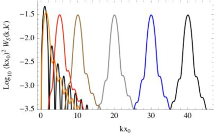
Figure 1: Window function $k^{2}x_{0}^{2}\,W_{\rm s}^{0}(k,k^{\prime})$, with $k^{\prime}x_{0}=0.1$, 1, 5, 10, 20, 30 and 40 (from left to right). For $k^{\prime}x_{0}\ll 1$ the window function is essentially independent of $k^{\prime}$ for $kx_{0}\ll 1$. Notice that even for large $k^{\prime}$ the window function does not become more localized around $k=k^{\prime}$ – the width of the window function around the peak is always limited by the size of the survey, $x_{0}^{-1}$.

The self-correlation window function $W_{\rm s}^{0}$ is positive everywhere, and is highly peaked around $k=k^{\prime}$ when $kx_{0}\gg 1$. However, in contrast to a delta-function, it only has support on a finite volume, and therefore it has the properties that both its width and its maximum height remain finite in the limit $k^{\prime}\rightarrow k$:

$$\displaystyle\lim_{k^{\prime}\to k}W_{\rm s}^{0}(k,k^{\prime}) = \frac{1}{256k^{6}x_{0}^{6}}\left(\cos kx_{0}+4kx_{0}\sin 4kx_{0}\right.$$ (66)

$$\left.-1-8k^{2}x_{0}^{2}+32k^{4}x_{0}^{4}\right)$$

$$+{\cal{O}}(k-k^{\prime})\;.$$

In fact, when $kx_{0}\gg 1$ the window function can be written as:

$$\displaystyle\lim_{k^{\prime}\to k}\;\displaystyle\lim_{kx_{0}\to\infty}W_{\rm s}^{0}(k,k^{\prime}) = \frac{1}{k^{2}x_{0}^{2}}\left[\frac{1}{8}-\frac{1}{36}(k-k^{\prime})^{2}x_{0}^{2}\right]$$ (67)

$$+{\cal{O}}(k-k^{\prime})^{3}\;.$$

This expression shows that even for arbitrarily small scales ($kx_{0}\gg 1$), the finite size of the survey limits the size of the volume in Fourier space inside which we can define a bandpower that is linearly independent from the other bandpowers. The minimal width of bandpowers in the small-scale limit is, from the formula above, $\Delta k_{\rm min}\sim 3/\sqrt{2}\,x_{0}^{-1}$.

One can also take the joint limits $k\to k^{\prime}$ and $k\to 0$, which then result in:

$$\displaystyle\lim_{k^{\prime}\to k}\;\displaystyle\lim_{kx_{0}\to 0}W_{\rm s}^{0}(k,k^{\prime})=\frac{1}{9}\left[1-\frac{2}{5}k^{2}x_{0}^{2}\right]+{\cal{O}}(k^{3})\;.$$ (68)

This limit shows why the classical approximation is inaccurate at large scales (small k): in that regime, the phase space window function is in fact independent of $k^{\prime}$ – i.e., on large scales the Fisher matrix is essentially an average over the phase space cells close to the origin. This result means that the first $k$-bin of a survey has to include all the modes $0<k\lesssim\sqrt{2/5}\,x_{0}^{-1}$. This is, of course, a manifestation of cosmic variance, which tells us that no survey can measure structure on scales larger than the size of the survey itself.

The preceding discussion implies that the optimal sizes of the bins both in the large-scale and in the small-scale regimes are always commensurate with the only other scale in the problem, $x_{0}^{-1}$. The only exception to this rule would be a spectrum $P(k)$ which has a very sharp and well-defined feature at some particular scale, such that the spectrum itself changes more rapidly than the window function near that scale.

Hence, to summarize the results of this Section, we have found that the Fisher matrix for the power spectrum in the case of a survey with a top-hat number density is given by:

$$F_{P}^{0}(k,k^{\prime})=\frac{(2\pi)^{3}}{2}\,U_{0}(k)\,U_{0}(k^{\prime})\,\frac{2}{\pi}x_{0}^{6}\,W_{\rm s}^{0}(k,k^{\prime})\;,$$ (69)

where $U_{0}(k)=N_{0}P(k)/[1+N_{0}P(k)]$ and $W_{\rm s}$ is given by Eq. (4.1).

Now, I will show that Eq. (69) is basically identical to the FKP Fisher matrix that was found, with a slightly different approach, by Hamilton [Hamilton (1997a)]. From that reference, considering only the lowest-order term in the series for the inverse of the covariance matrix, we get that:

$$F_{P}^{\rm(FKP)}(k,k^{\prime})=\frac{1}{2}\int\frac{d^{2}\hat{k}}{4\pi}\,\frac{d^{2}\hat{k}^{\prime}}{4\pi}\,|\tilde{U}(\vec{k}+\vec{k}^{\prime})|^{2}\;,$$ (70)

where:

$$\tilde{U}(\vec{k})=\int d^{3}x\,e^{i\vec{k}\cdot\vec{x}}\,U(\bar{k},x)=\int d^{3}x\,e^{i\vec{k}\cdot\vec{x}}\,\frac{N(x)P(\bar{k})}{1+N(x)P(\bar{k})}\;.$$ (71)

In the expression above, $\bar{k}$ corresponds to a “trial” wavenumber that should be chosen a posteriori in order to maximize the Fisher matrix (and minimize the covariance) for the bandpower that is being estimated. The scale $\bar{k}$ is in fact inherited from the inversion of the covariance matrix, under the approximation that it is diagonal. It is not entirely clear what sets the correct choice of $\bar{k}$, but it has been common practice to take $\bar{k}\to(k+k^{\prime})/2$ [Hamilton (1997a, b); Tegmark (1997)].

Under the assumption of isotropy and with a top-hat effective number density $N(x)=N_{0}\theta(x_{0}-x)$, it is trivial to compute $\tilde{U}$ in the classical limit:

$$\tilde{U}(\bar{k};k) = 4\pi\,U_{0}(\bar{k})\,k^{-3}\left[\sin kx_{0}-kx_{0}\cos kx_{0}\right]$$

$$= 4\pi\,U_{0}(\bar{k})\,k^{-3}\,(kx_{0})^{2}j_{1}(kx_{0})\;.$$

Substituting this expression into Eq. (70) we find that the integral is exact, and the result is in fact:

$$F_{P}^{0\,{\rm(FKP)}}(k,k^{\prime})=\frac{(2\pi)^{3}}{2}\,U_{0}^{2}(\bar{k})\,\frac{2}{\pi}x_{0}^{6}\,W_{\rm s}^{0}(k,k^{\prime})\;.$$ (73)

Now compare Eqs. (69) and (73): the phase space window function is precisely the same in the two expressions, and the only difference is that the latter equation takes $k=k^{\prime}=\bar{k}$ in $U_{0}$. This is a good approximation only if the $k$ bins are sufficiently large, in which case the binned window function is very nearly diagonal.

4.2 FKP formulas: the stationary phase limit

Now, let’s compare the analytical result of the previous section with the corresponding FKP formulas (which are in the stationary phase limit). Because of the Dirac delta function in the FKP Fisher matrix, it is more convenient to compare the averages over bins $k_{i}$:

$$F_{P,ij} = \int_{\tilde{V}_{i}}\frac{d^{3}k}{(2\pi)^{3}}\,\int_{\tilde{V}_{j}}\frac{d^{3}k^{\prime}}{(2\pi)^{3}}\,F_{P}(k,k^{\prime})$$

$$\approx \frac{\tilde{V}_{i}}{(2\pi)^{3}}\,\frac{\tilde{V}_{j}}{(2\pi)^{3}}\,F_{P}(k=k_{i},k^{\prime}=k_{j})$$

$$= \frac{1}{2(2\pi)^{3}}\,U_{0}(k_{i})\,U_{0}(k_{j})\,\tilde{V}_{i}\,\tilde{V}_{j}\,\frac{2}{\pi}\,x_{0}^{6}\,W_{\rm s}^{0}(k_{i},k_{j})\;,$$

where $\tilde{V}_{i}=4\pi k_{i}^{2}\Delta k_{i}$ is the volume of the shell in Fourier space around the $i$-th bin, and in the last expression I assumed that the binning is small enough that $F_{P}$ does not vary too much inside the bin.

The FKP Fisher matrix in the classical limit can be obtained directly from Eq. (4) by taking the SP approximation, ${\cal{W}}(k,x;k^{\prime},x^{\prime})\rightarrow k^{-2}\delta_{D}(k-k^{\prime})\,x^{-2}\delta_{D}(x-x^{\prime})$. For our top-hat profile, the FKP Fisher matrix for the power spectrum in the classical limit is:

$$\lim_{\rm class}F_{P,ij}=\frac{(2\pi)^{3}}{2}\,U_{0}^{2}(k_{i})\,\delta_{ij}\,\frac{\tilde{V}_{i}\,V_{0}}{(2\pi)^{6}}\;,$$ (75)

where $V_{0}=4\pi\,x_{0}^{3}/3$ is the total volume of the survey (in position space, naturally).

It is possible to compare the full expression for the Fisher matrix with its classical limit, in a way which is completely independent of the phase space weighting function $U_{0}$ – and, therefore, in a way that does not depend on either the effective density $N_{0}$ or the fiducial power spectrum $P(k)$. In fact, all we need to do is to compare the adimensional matrices associated with the phase space volume:

$${\cal{V}}_{ij}^{\rm class}=\tilde{V}_{i}\;V_{0}\;\delta_{ij}\quad\quad v.\quad\quad{\cal{V}}^{s}_{ij}=\tilde{V}_{i}\;\tilde{V}_{j}\;\frac{2}{\pi}\;x_{0}^{6}\;W_{\rm s}^{0}(k_{i},k_{j})\;,$$ (76)

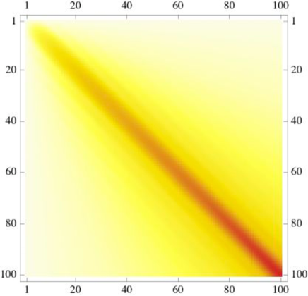
Figure 2: Self-correlation phase space volume matrix ${\cal{V}}^{s}_{ij}$ with 100 equally-spaced bins between $kx_{0}=0$ and $kx_{0}=50$.

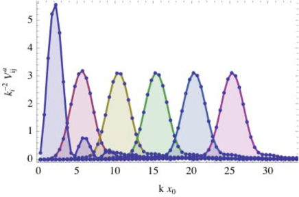
Figure 3: Rows $i$ of the matrix $(k_{i}x_{0})^{-2}{\cal{V}}^{s}_{ij}$ shown in Fig. 2for the bins $kx_{0}=0.5$, 5, 10, 15, 20 and 25 ($j=1$, 6, 11, 16 $\ldots$ 51). Since $\tilde{V}_{i}$ is proportional do $k_{i}^{2}$, I plot the volume times an adimensional pre-factor of $(k_{i}x_{0})^{-2}$. Above $kx_{0}\sim 10$ the rows of the volume matrix are essentially self-similar after normalizing for the pre-factor of $(kx_{0})^{-2}$.

In Fig. 2 I plot the self-correlation phase space volume matrix ${\cal{V}}^{s}_{ij}$, binned in 100 equally spaced intervals of $\Delta k=0.5x_{0}^{-1}$ between $k=0$ and $kx_{0}=50$. In this 2D representation of the phase space volume matrix, darker colors denote higher values of phase space volume. Obviously, the classical counterpart of this matrix is the diagonal matrix ${\cal{V}}_{ij}^{class}$. In Fig. 3 I plot some of the rows of the volume matrix, to show how they are spread out over the $k$ bins. In the classical limit, each curve would be a Dirac delta-function centered on $k=k^{\prime}$.

In Fig. 4 I compare the entries of the full phase space volume, ${\cal{V}}_{ij}$, with the normalization provided by the classical (FKP) approximation, ${\cal{V}}_{ij}^{\rm class}$. The upper set of points (blue in color version) denote the diagonal elements of the phase space volume in the classical approximation. The lower set of points (yellow in color version) denote the diagonal elements of the full phase space volume matrix, ${\cal{V}}_{ii}$. Also plotted are the traces of the rows of the volume matrix, ${\cal{V}}_{i}=\sum_{j}{\cal{V}}_{ij}$ (middle set of points, red in color version). Since the phase space window function ${\cal{W}}$ is in fact normalized to unity over the whole volume of phase space, these traces should be equal to their classical limit counterparts. Fig. 4 shows that, indeed, the normalization of the full phase space volume matrix is very well approximated by the classical approximation on all but the largest scales – the difference is essentially due to the finite size of the bins. The fall-off seen on very small scales (the highest values of $k$) is just an artifact of cutting off the bins at the edge ($kx_{0}=50$ in our example).

Inspection of Figs. 2-3 shows that, by increasing the size of the $k$ bins, the full Fisher matrix can be well approximated by the classical limit expression. Under these conditions the bandpowers are then approximately uncorrelated – although we should always keep in mind that coarse-graining the Fisher matrix leads to loss of information, and that this lack of correlation only applies for bins of order at least $\Delta k\sim 5x_{0}^{-1}$ in our example of a top-hat effective density. To put that into perspective, for a uniform Hubble-size ($cH_{0}^{-1}\sim h^{-1}2997$ Mpc) galaxy survey the bins would need to be only as large as $\Delta k\sim 3.10^{-4}$ $h$ Mpc^-1 for this approximation to be applicable, and for a survey spanning a tenth of a Hubble volume the $k$ bins would need to be greater than $\Delta k\sim 3.10^{-3}$ $h$ Mpc^-1. As a concrete example, consider the analysis of baryon acoustic oscillations on the SDSS-7 performed in Percival et al. (2010): if the volumetric galaxy density of that dataset were homogeneous and isotropic, the minimal size of the bins such that the bandpowers are approximately uncorrelated should be of order $\Delta k\sim 0.007$ $h$ Mpc^-1. However, in Figs. 1 and 3 of that paper the bins are spaced only by $\Delta k\sim 0.004$ $h$ Mpc^-1, which means that the datapoints shown in those figures are highly correlated. For their statistical analysis, Percival et al. (2010) fitted cubic splines on nodes separated by $\Delta k\sim 0.05$ $h$ Mpc^-1, which gives an effective bin size of approximately a quarter of that separation, i.e., $\Delta k_{eff}\sim 0.0125$ $h$ Mpc^-1, which is close to the limit I computed above assuming a top-hat density profile of galaxies. Using a more realistic distribution of galaxies as a function of redshift and angular position in the sky would only make this problem worse.

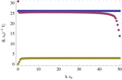
Figure 4: Diagonal elements of the full phase space volume matrix (lower points, yellow in color version), compared to the same volume in the classical (FKP) approximation (upper points, blue in color version). I also show the traces of each individual line of the phase space volume matrix (middle points, red in color version), which are very well approximated by the diagonal elements of the volume matrix in the classical approximation, simply because the phase space window function is normalized (the end points are off due to the edges of those bins having been cut-off). I have employed 100 bins between $kx_{0}=0$ and $kx_{0}=50$.

As mentioned above, one should keep in mind that by increasing the size of the bin we lose some amount of information by washing out the Fisher matrix. On the other hand, for practical and numerical purposes it is inefficient to keep an excessively large number of bins. In that sense, it is interesting to examine how many linearly independent modes are encoded in the Fisher matrix, by making a principal component analysis (PCA) on it. The result of the PCA decomposition fn our Fisher matrix with 100 equally spaced bins is presented in Fig. 5, where the principal values are plotted as a function of $k$ for the 100 bins. Fig. 6 shows the eigenvalues corresponding to the principal values. From Fig. 6 it can be seen that only about 35 components are relevant for this Fisher matrix, and from Fig. 5 we see that the highest-ranked ones probe the small scales (large $k$), whereas the lowest-ranked amongst the 35 non-trivial principal components span the large scales (small $k$). The 65 lowest-ranking principal values have negligible eigenvalues, and it is clear that they carry no information whatsoever. This is an indication that the optimal average size of the bins in the case of a top-hat survey should be at most of the order of $\Delta k\sim 50\,x_{0}^{-1}/35\simeq 1.4\,x_{0}^{-1}$. However, in that case one should be careful to include the cross-correlations between the different bandpowers, as not doing so would lead to an overestimation of the constraints.

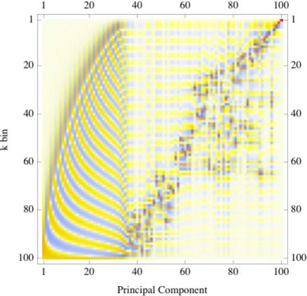
Figure 5: Principal components of the Fisher matrix, binned in 100 equally spaced intervals between $kx_{0}=0$ and $kx_{0}=50$. The horizontal axis corresponds to each principal component, ranked by their eigenvalues, and the vertical axis (from top to bottom) corresponds to the $k$ bins.

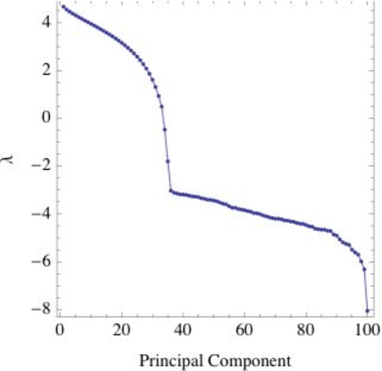
Figure 6: Eigenvalues of the principal components of the Fisher matrix. It is clear from both Fig. 5 and 6 that there are only about 35 principal values with non-negligible eigenvalues, which means that only as many linearly independent bandpowers can be estimated from the data. The plots also show that, among the non-negligible principal components, the highest-ranked correlate with large values of $k$, and the lowest-ranked involve essentially the small-$k$ bins.

4.3 Analytical solution for two species of tracers with top-hat density profiles, including the cross-correlations

Now I will generalize the results of the previous section to the case where we have two species of tracers. The main distinction with the previous sections is that now the total number density is the sum of two different top-hats, $N(x)=N_{1}(x)+N_{2}(x)$, where $N_{\mu}(x)=N_{\mu}\,\theta(x_{\mu}-x)$. Here I will assume that the survey of species 1 is dense but shallow, and the survey of species 2 is sparse but deep, so $N_{1}>N_{2}$ and $x_{1}<x_{2}$. This would be the case, e.g., of a homogeneous survey of luminous red galaxies limited to $z\lesssim 1$, and a survey of quasars or Ly-$\alpha$ absorption systems limited to $z\lesssim 3$.

With this in mind, we can write the phase space weighting function $U_{1}$ of the previous Section as:

$$U_{1}(k,x) = \frac{N_{1}\theta(x_{1}-x)P(k)}{1+[N_{1}\theta(x_{1}-x)+N_{2}\theta(x_{2}-x)]P(k)}$$

$$= \frac{N_{1}P(k)}{1+N_{12}P(k)}\theta(x_{1}-x)\;,$$

where $N_{12}=N_{1}+N_{2}$ is the total effective number density for $0<x\leq x_{1}$. For the tracer species 2 the weighting function is expressed as:

$$U_{2}(k,x) = \frac{N_{2}\theta(x_{2}-x)P(k)}{1+[N_{1}\theta(x_{1}-x)+N_{2}\theta(x_{2}-x)]P(k)}$$

$$= \left[\frac{N_{2}P(k)}{1+N_{12}P(k)}-\frac{N_{2}P(k)}{1+N_{2}P(k)}\right]\theta(x_{1}-x)$$

$$+\frac{N_{2}P(k)}{1+N_{2}P(k)}\theta(x_{2}-x);.$$

Clearly, then, we can redefine the two effective densities so that they reflect the two distinct top-hats. Collecting the amplitudes of each individual top-hat profile, we obtain:

$$U_{1}^{\prime}(k,x) = \left[\frac{N_{12}P(k)}{1+N_{12}P(k)}-\frac{N_{2}P(k)}{1+N_{2}P(k)}\right]\,\theta(x_{1}-x)$$

$$\equiv U_{1}^{\prime}(k)\,\theta(x_{1}-x)\;,$$

$$U_{2}^{\prime}(k,x) = \frac{N_{2}P(k)}{1+N_{2}P(k)}\,\theta(x_{2}-x)$$

$$\equiv U_{2}^{\prime}(k)\,\theta(x_{2}-x)\;.$$

Therefore, when computing the total Fisher matrix for two species of tracers one should include the two self-correlation Fisher matrices, as discussed in the previous section, using either $U_{1}^{\prime}(k)$ for the self-correlation of species 1, or $U_{2}^{\prime}(k)$ for the self-correlation of species 2. In addition, we must also include the Fisher matrix for the cross-correlation between the two effective top-hats of Eqs. (4.3)-(4.3), which I discuss now.

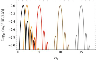
Figure 7: Cross-correlation phase space window function $k^{2}x_{1}^{2}\,W_{\rm c}^{12}(k,k^{\prime})$, with $x_{2}=2x_{1}$. The modes plotted are, from left to right, $k^{\prime}x_{1}=1$, 2, 5, 10, and 15. As was the case for the self-correlation window function, for $k^{\prime}x_{1}\ll 1$ the window function is essentially independent of $k^{\prime}$. The most important difference between the two window functions is that the cross window function can become negative – notice that I have plotted the log of the absolute value of $k^{2}W_{\rm c}$, but the positive values are always found at the peak of the window function, and the spikes to negative infinity mark the transition from positive to negative values or vice-versa. The width of the window function around the peak is given by the inverse of the largest length scale of the survey (in this example, $x_{2}$).

The Fisher matrix for the cross-spectrum arises from the cross-correlation between two species of tracers of large-scale structure. From Eq. (4), and according to the discussion of Section 2, the Fisher matrix for the cross-correlation between the top-hat of radius $x_{1}$ and the top-hat density of radius $x_{2}$ is given by:

$$F^{12}_{P}(k,k^{\prime}) = 8\pi^{2}\,U_{1}^{\prime}(k)\,U_{2}^{\prime}(k^{\prime})\,\sum_{\ell}(2\ell+1)$$

$$\times\int_{0}^{x_{1}}dx\,x^{2}\,j_{\ell}(kx)\,j_{\ell}(k^{\prime}x)\,$$

$$\times\int_{0}^{x_{2}}dx^{\prime}\,x^{\prime 2}\,j_{\ell}(kx^{\prime})\,j_{\ell}(k^{\prime}x^{\prime})\;.$$

Using the same derivation that was used to arrive at Eq. (62), I get:

$$W_{\rm c}^{1\,2}(k,k^{\prime}) = \frac{1}{(k^{2}-k^{\prime 2})^{2}\,x_{1}^{2}\,x_{2}^{2}}$$

$$\times\sum_{\ell}(2\ell+1)\,g_{\ell}^{1}(k,k^{\prime})\,g_{\ell}^{2}(k,k^{\prime})\;,$$

where:

$$g^{i}_{\ell}(k,k^{\prime})=k\,x_{i}\,j_{\ell}^{\prime}(kx_{i})\,j_{\ell}(k^{\prime}x_{i})-k^{\prime}x_{i}\,j_{\ell}^{\prime}(k^{\prime}x_{i})\,j_{\ell}(kx_{i}).$$ (83)

Since $g_{\ell}^{i}(k,k^{\prime})$ is of order ${\cal{O}}(k-k^{\prime})$ in the limit $k^{\prime}\to k$, the cross window function is well-behaved everywhere. The most important distinction between the self-correlation window function $W_{\rm s}$ and the cross-correlation one, $W_{\rm c}$, is that the former is always positive, whereas the latter is positive at its peak (at $k^{\prime}=k$), but presents damped oscillations between positive and negative values away from the peak. Another important difference between the self-correlation and the cross-correlation window functions is that I was able to find an analytical expression for the former, but not for the latter, which is left in the form of the infinite sum, Eq. (4.3). The situation is not as dire as it may seem, since the spherical Bessel functions $j_{\ell}(z)$ are highly peaked around $z\sim\ell$, and Limber-type approximations allow us to cut off the infinite sum to a small number of terms with minimal loss of precision. In Fig. 7 I plot some of the modes of the cross window function in the case $x_{2}=2x_{1}$.

The full Fisher matrix for the power spectrum in the case of two top-hat profiles is therefore given by the combination of the self-correlation and the cross-correlation terms corresponding to the two top-hats above, with amplitudes $U_{1}^{\prime}(k)$ and $U_{2}^{\prime}(k)$. The explicit expression is:

$$F_{P}(k,k^{\prime}) = 8\pi^{2}\,\left\{x_{1}^{6}\,U_{1}^{\prime}(k)\,U_{1}^{\prime}(k^{\prime})\,W_{\rm s}^{1}(k,k^{\prime})\right.$$

$$+x_{2}^{6}\,U_{2}^{\prime}(k)\,U_{2}^{\prime}(k^{\prime})\,W_{\rm s}^{2}(k,k^{\prime})$$

$$+\,x_{1}^{3}x_{2}^{3}\,\left[U_{1}^{\prime}(k)\,U_{2}^{\prime}(k^{\prime})\,W_{\rm c}^{12}(k,k^{\prime})\right.$$

$$\left.\left.+U_{2}^{\prime}(k)\,U_{1}^{\prime}(k^{\prime})\,W_{\rm c}^{21}(k,k^{\prime})\right]\right\}\;,$$

and the binned Fisher matrix is, therefore:

$$F_{P,ij} = \frac{1}{2(2\pi)^{3}}\,\left\{U_{1,i}^{\prime}\,U_{1,j}^{\prime}\,{\cal{V}}_{ij}^{s\,(1)}+\,U_{2,i}^{\prime}\,U_{2,j}^{\prime}\,{\cal{V}}_{ij}^{s\,(2)}\right.$$

$$\left.+\,\left[U_{1,i}^{\prime}\,U_{2,j}^{\prime}+U_{2,i}^{\prime}\,U_{1,j}^{\prime}\right]\,{\cal{V}}_{ij}^{c}\right\}\;,$$

where ${\cal{V}}^{c}$ is defined in terms of the cross-correlation window function $W_{\rm c}$ in the same way as ${\cal{V}}^{s}$ was defined in terms of $W_{\rm s}$ in Eq. (76):

$${\cal{V}}_{ij}^{c}=\tilde{V}_{i}\,\tilde{V}_{j}\,\frac{2}{\pi}\,x_{1}^{3}\,x_{2}^{3}\,W_{\rm c}(k_{i},k_{j})\;.$$ (86)

The SP approximation to the full Fisher matrix can be reached directly from Eq. (4) by taking the limit ${\cal{W}}(k,x;k^{\prime},x^{\prime})\to k^{-2}\delta_{D}(k-k^{\prime})\,x^{-2}\delta_{D}(x-x^{\prime})$, and then integrating over the volumes of the $k$ bins:

$$F_{P,ij}^{\rm FKP} = \frac{1}{2(2\pi)^{3}}\,\tilde{V}_{i}\,\delta_{ij}$$

$$\times\left[\frac{4\pi}{3}\,x_{1}^{3}\,U_{12,i}^{2}+\frac{4\pi}{3}\,(x_{2}^{3}-x_{1}^{3})\,U_{2,i}^{\prime 2}\right]\;,$$

where $U_{12,i}=N_{12}P(k_{i})/[1+N_{12}P(k_{i})]=U_{1}^{\prime}+U_{2}^{\prime}$. The relevant difference with respect to the analytical expression in the classical limit is that, because of the SP approximation, all the signal from the cross-correlation between 1 and 2 is already implicitly included in the amplitudes $U_{12}$ and $U_{2}^{\prime}$. This becomes clearer if we rewrite the SP limit of the full Fisher matrix as:

$$F_{P,ij}^{\rm FKP} = \frac{1}{2(2\pi)^{3}}\,\tilde{V}_{i}\,\delta_{ij}\,\frac{4\pi}{3}$$

$$\times\left[x_{1}^{3}\,U_{1,i}^{\prime 2}+x_{2}^{3}U_{2,i}^{\prime 2}+x_{1}^{3}\left(U_{12,i}^{2}-U_{1,i}^{\prime 2}-U_{2,i}^{\prime 2}\right)\right]$$

$$= \frac{1}{2(2\pi)^{3}}\,\tilde{V}_{i}\,\delta_{ij}\,\frac{4\pi}{3}$$

$$\times\left[x_{1}^{3}\,U_{1,i}^{\prime 2}+x_{2}^{3}\,U_{2,i}^{\prime 2}+2\,x_{1}^{3}\,U_{1,i}^{\prime}\,U_{2,i}^{\prime}\right]\;.$$

Compare now this last expression with Eq. (4.3). The self-correlation term for species 1 has already been analyzed in the previous sections, and the self-correlation term for species 2 is precisely the same, except for the scaling $k\to k\times x_{1}/x_{2}$. The comparable cross-correlation terms are $\tilde{V}_{i}V_{1}\delta_{ij}$ and ${\cal{V}}_{ij}^{c}$, as defined in Eq. (86).

I show the cross-correlation phase space volume in Figs. 8 and 9. On Fig. 8, the rows of the volume matrix are plotted for the first few $k$ bins. As discussed above, the phase space window function (and, therefore, the volume matrix) can be negative for the cross-correlation term. Comparing Figs. 3 and 9 we see that the cross-correlation volume matrix is narrower around the diagonal. However, this is a simple consequence of the inclusion of the second species of tracer, whose top-hat profile has a radius $x_{2}=2x_{1}$. Naturally, the width of the cross-correlation volume matrix in $k$ bins is dominated by the inverse of the largest scale, which in this example is $\Delta k\sim x_{2}^{-1}=0.5x_{1}^{-1}$ .

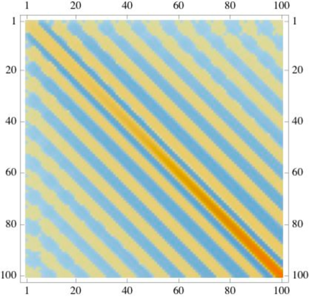
Figure 8: Cross-correlation phase space volume matrix ${\cal{V}}^{c}_{ij}$, with 100 equally-spaced bins between $kx_{1}=0$ and $kx_{1}=50$, and assuming $x_{2}=2x_{1}$.

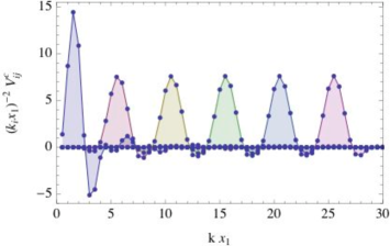
Figure 9: Rows of $k_{i}^{2}\,{\cal{V}}^{c}_{ij}$ for the bins $kx_{1}=0.5$, 5, 10, 15, 20 and 25 (from left to right, respectively).

In Fig. 10 I compare the phase space volume with its SP approximation, for both the self-correlation terms and for the cross-correlation as well. In order to compare the volume matrices on an equal footing, I have normalized the volume of species 2 to the volume of species 1. In the upper panel I have plotted $\tilde{V}_{i}V_{1}$, as well as the traces of each row of the volume matrices, $\sum_{j}{\cal{V}}_{ij}^{s(1)}$, $V_{1}/V_{2}\times\sum_{j}{\cal{V}}_{ij}^{s(2)}$ and $\times\sum_{j}{\cal{V}}_{ij}^{c}$. From the upper panel we can verify that there is good agreement between the SP approximation and the analytical result in the classical approximation at intermediate scales, where the analytical result is only $\sim$ 2-3% below the SP approximation. This means that, by taking large enough $k$-bins one can recover the FKP result for the Fisher matrix from the result in the classical approximation. Only at the very largest scales (the single bin between $0<kx_{1}\leq 0.5$) the SP approximation fails, and the FKP Fisher matrix understates the constraining power of the survey.

The lower panel of Fig. 10 shows the ratios of the diagonals of the phase space volume matrices to the traces of their respective rows – which is a measure of how diagonal those matrices are. Tracer species 1, which occupies the smallest volume, is the least diagonal, and tracer species 2, which spans length scales roughly double those of species 1, has a more diagonal Fisher matrix, by a factor of two, approximately. The cross-correlation Fisher matrix, in fact, appears to be the most diagonal of the Fisher matrices. However, that is partly an artifact coming from the wings of the cross-correlation window function, which are negative – see Fig2. 8-9. When we account for this (by, e.g., using the squares of the window functions as the normalization), the cross-correlation Fisher matrix comes out to be approximately as diagonal as the self-correlation Fisher matrix of the tracer species with the largest volume – in our case, species 2.

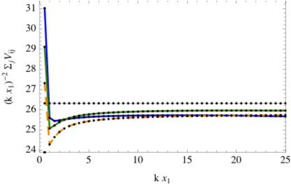
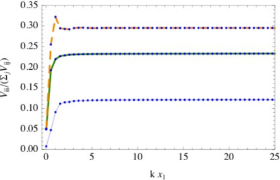
Figure 10: Upper panel: the horizontal row of points are the classical and SP approximations to the phase space volume matrix for the cross-correlation between tracer species 1 and 2. The lower and upper solid lines (blue and green in color version) correspond to the trace of the rows of the self-correlation phase space matrices of species 1 and 2, respectively – i.e., $\sum_{j}{\cal{V}}_{ij}^{s(1,2)}$. The dashed line (orange in color version) corresponds to the trace of the cross-correlation phase space matrix. Lower panel: ratios of the diagonal elements of the phase space volume matrices to their traces, ${\cal{V}}_{ii}/\sum_{j}{\cal{V}}_{ij}$. From the lower to the upper lines, self-correlation of species 1 (lower solid line, blue in color version), self-correlation of species 2 (middle solid line, green in color version), and cross-correlation ${\cal{V}}_{ii}^{c}$ (upper dashed line, orange in color version). I employ 100 bins between $kx_{1}=0$ and $kx_{1}=50$.

It is also useful to perform a PCA analysis on the cross-correlation phase space volume, as was done for the self-correlation volume in the previous section. On Fig. 11 I show the principal components of ${\cal{V}}^{c}$ as a function of the $k$ bins. On Fig. 12 I show the eigenvalues of the principal values for the self-correlations of species 1 and 2, as well as the cross-correlation between the two species.

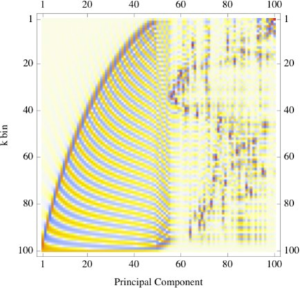
Figure 11: Principal components of the cross-correlation Fisher matrix for the power spectrum, binned in 100 equally spaced intervals between $kx_{0}=0$ and $kx_{0}=50$. The horizontal axis corresponds to each principal component, ranked by their eigenvalues, and the vertical axis (from top to bottom) corresponds to the $k$ bins.

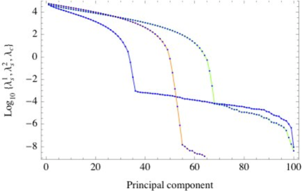
Figure 12: Eigenvalues of the principal components of the Fisher matrices for the self-correlation of tracer species 1 with itself (left line and points, blue in color version), for the self-correlation of species 2 with itself (right line, green in color version), and for the cross-correlation between the two species (middle line, orange in color version).

The results of this Section can be easily generalized to an arbitrary number of species of tracers, and to any (isotropic) number density – not only uniform densities.

5 Discussion

In this paper I have shown how to compute the Fisher matrix for galaxy surveys, including the cross-correlations between different cells in position space and in Fourier space. In the stationary phase approximation these cross-correlations are discarded – Hamilton [Hamilton (1997a, c)] refers to this case as the “classical limit”.

I have also shown how to obtain the Fisher matrix for multiple species of tracers of large-scale structure from the covariance of counts of galaxies in cells. The final formulas, after taking the classical and SP limits, generalizes the results previously obtained by Percival et al. (2003); White et al. (2008); McDonald & Seljak (2008). However, I have also obtained the Fisher matrix using only the classical limit, which solves some (probably minor) inconsistencies of those formulas. I have also shown that, in order to invert the covariance matrix for the full dataset with all species of tracers, all that is needed is the inversion of a single matrix (or operator), $\hat{\cal{C}}$, and not the inversion of a large set of linear equations – see Eq. (21) and the following discussion. The main results are summarized by Eqs. (40)-(45), and their classical limits are shown in Eqs. (3.3)-(3.3).

The full Fisher matrix in the classical approximation can be expressed entirely in terms of the phase space weighting functions $U_{\mu}(\vec{k},\vec{x})=N_{\mu}(\vec{x})\,P(\vec{k})/[1+N(\vec{x})\,P(\vec{k})]$, where $N_{\mu}(\vec{x})=\bar{n}_{\mu}B_{\mu}^{2}$ is the effective density of the tracer species $\mu$. These weighting functions are basically the FKP pair-weights. These results make the case that, just as $P(\vec{k})$ is the density of modes in Fourier space, and $N(\vec{x})=\sum_{\mu}N_{\mu}$ plays the role of the total effective density of tracers in position space, the quantity $\frac{1}{2}U^{2}(\vec{k},\vec{x})$ can be interpreted as the density of information in phase space. The Fisher information matrix for the power spectrum is simply the sum (or trace) of the information over position-space volume [i.e., the effective volume $V_{eff}(\vec{k})$], and the Fisher matrix for the bias is the sum (or trace) of the information over the Fourier-space volume [what I have called here $\tilde{V}_{eff}(\vec{x})$]. The elements of the Fisher matrix which mix the power spectrum estimation at $\vec{k}$ with the bias estimation at $\vec{x}$ are given simply in terms of $\frac{1}{2}U^{2}$ (the density of information), times the phase space volume occupied by the bins at $\vec{k}$ and at $\vec{x}$. In a forthcoming paper (Abramo 2011, to appear) I will show how to use this result to jointly estimate the power spectrum and the bias (together with the matter growth function) from the same dataset, without introducing hidden priors; and conversely, how to properly include priors in these estimations.

Acknowledgements – I would like to thank Ravi Sheth for bringing to my attention some of the puzzles that ultimately led to this work; many thanks also to G. Bernstein, Y.-C. Cai, A. Hamilton, B. Jain and M. Strauss for useful comments and/or discussions. I would like to thank the Department of Physics and Astronomy at the University of Pennsylvannia, as well as the Department of Astrophysical Sciences at Princeton University, for their warm hospitality. This work was supported by both FAPESP and CNPq of Brazil.

References

Abbott et al. (2005)
Abbott, T. et al., 2005, astro-ph/0510346.
Abell et al. (2009)
Abell, P. et al., 2009, 0912.0201
Abramo et al. (2011)
Abramo, L. R. et al., 2011, 1108.2657
Adelman-McCarthy et al. (2008a)
Adelman-McCarthy, J. K. et al., 2008a, VizieR Online Data Catalog 2282, 0
Adelman-McCarthy et al. (2008b)
Adelman-McCarthy, J. K. et al., 2008b, ApJS 175, 297
Albrecht et al. (2009)
Albrecht, A. et al., 2009, 0901.0721
Benítez et al. (2009)
Benítez, N. et al., 2009, ApJ 691, 241
Bernstein (1994)
Bernstein, G. M. 1994, Astroph. J. 424, 569