Denaturation of Circular DNA: Supercoil Mechanism

Abstract

The denaturation transition which takes place in circular DNA is analyzed by extending the Poland-Scheraga model to include the winding degrees of freedom. We consider the case of a homopolymer whereby the winding number of the double stranded helix, released by a loop denaturation, is absorbed by supercoils. We find that as in the case of linear DNA, the order of the transition is determined by the loop exponent $c$. However the first order transition displayed by the PS model for $c>2$ in linear DNA is replaced by a continuous transition with arbitrarily high order as $c$ approaches 2, while the second-order transition found in the linear case in the regime $1<c\leq 2$ disappears. In addition, our analysis reveals that melting under fixed linking number is a condensation transition, where the condensate is a macroscopic loop which appears above the critical temperature.

I Introduction

Thermal denaturation of DNA is a process by which the two strands of the molecule unbind upon heating. A good understanding of the underlying physics is relevant to certain biological systems (e.g., thermophilic organisms DSD1992 ; HS2004 ) as well as synthetic technologies  WB1985 such as polymerase chain reaction (PCR) HM1994 ; HM1996 and DNA microarrays CH2006 . The unbinding transition takes place at a specific temperature, coined melting or denaturation temperature, which can be defined experimentally as the temperature at which the fraction of unbound base pairs reaches, say, half of its maximal value. For a relatively homogenous DNA chain composed largely of A-T (or G-C) pairs, melting takes place through a very sharp increase in the fraction of broken bases, suggesting a first-order phase transition in an idealized homogeneous system. This phase transition has been investigated by means of various theoretical approaches developed in recent decades PB1989 ; Fisher1966 ; PS1966 ; DPB1993 ; KMP2000 ; WM1972 ; Ben1980 ; Ben1992 ; BM2000 ; PMD2007 ; MS1994b ; NG2006 .

A prototypical model employed in theoretical studies of this phenomenon is the Poland-Scheraga (PS) model PS1966 in which a microscopic configuration of the DNA molecule is described by an alternating succession of bound segments (dsDNA) and denaturated loops (ssDNA). As the temperature is increased the total length of the bound segments decreases, eventually vanishing at the melting transition. The transition is a result of the competition between the enthalpy associated with the hydrogen bonding of the matching bases, and the entropy of loops. The loop entropy has the asymptotic form $\sim s^{l}/l^{c}$ for large loop size $l$, where $s$ is a geometric, non-universal constant and $c$ is a universal exponent. The original PS model makes the simplifying assumption that the binding energy is the same for all base pairs, in which case the nature of the transition depends only on the parameter $c$ PS1966 . For $c\leq 1$ no transition takes place and the two strands are bound at all temperatures. For $1<c\leq 2$ the model exhibits a second-order melting transition where the average loop length increases and becomes macroscopic of order $L$ as the critical point is approached from below. For $c>2$ the transition is first order and the average loop length remains $O(1)$ for $T\leq T_{c}$. For $T>T_{c}$ a macroscopic loop, formed abruptly at $T_{c}$, is present. In $d=3$ dimensions and with exclusion interaction properly taken into account, one obtains $c\approx 2.12$ KMP2000 ; KMP2002 ; COS2002 and the transition is predicted to be first order. The PS model has later been extended to address the sequence dependence of the melting transition in heteropolymeric DNAs Meltsim .

The DNA molecule is helical, and therefore denaturation entails unwinding of the two strands around one another. The PS model ignores this fact, as the elastic strain can be relaxed by the rotation of the chain ends. However there are cases where the helicity can not be ignored. For example, bacteria have circular DNAs (plasmids) whose linking number (the number of times one strand winds around the other) is a topological invariant. Similarly, certain single-molecule experiments require the chain ends to be rotationally constrained. In such cases, unwinding of a loop is possible only if some extra linking number can be absorbed by the rest of the molecule.

Previous studies that model denaturation of circular DNA proposed two mechanisms by which bound DNA segments may host extra linking number released by opening a loop: (a) increasing the twist (the excess stacking angle integrated along the centerline) RB2002 ; GOY2004 ; or (b) increasing the writhe (which is a function of the centerline configuration itself), for example by forming a supercoil KOM09 ; KOM2010 ; KAS2010 . The AFM images of thermally denatured DNA circles adsorbed on a mica surface suggest that supercoils do form in conjunction with denaturation loops YI2002 . Numerical studies similarly point at the writhe as the dominant mechanism for absorbing the extra linking number in long DNA circles KAS2010 .

In this paper we study in detail the case of supercoils. In an earlier work this model has been studied at temperatures below the melting point KOM09 , by means of a grand canonical treatment where the expectation value of the linking number is fixed. Here we generalize this approach and further consider the high-temperature denatured phase in order to study the nature of the melting transition. The validity of our results is then verified by a direct calculation within a canonical formalism where the linking number is strictly conserved. This approach allows us to point out an inconsistency in the assumed analogy with the PS model in Ref.KOM09 . Finally, we find the following phase diagram: For $c\leq 2$ the model exhibits no phase transition and a steady increase of loop fraction with temperature. For $c>2$ a continuous transition of order $\left\lceil\frac{c-1}{c-2}\right\rceil$ takes place, where $\left\lceil q\right\rceil$ is the upper integer value of $q$. The order of the transition tends to infinity as $c\to 2$.

The paper is arranged as follows: In section II, we present the model. In section III, the denaturation transition is first established in the grand-canonical ensemble, where we introduce a regularization scheme used earlier in KMP2002 . This procedure allows us to draw an analogy between the high-temperature phase and a Bose-Einstein condensate where a critical fluid (microscopic loops) coexists with a condensate (a single macroscopic loop). In section IV, we reinvestigate the model within the canonical formalism: while we observe a general agreement between the two ensembles, we also point out a difference between the corresponding condensates that suggests the inequivalence of the two ensembles for finite systems in the present context. Finally, in section V, we present some concluding remarks and discuss possible future directions.

II Model definition

Following KOM09 we extend the PS model to include supercoiled DNA segments. Thus, a microscopic configuration is composed of an alternating arrangement of three types of segments:

1. a bound segment, in which base pairs are intact but no supercoiling takes place. Following the PS model, we neglect the entropic contribution of such a segment, so that its Boltzmann weight is solely determined by the binding energy $E_{b}<0$ and the segment length $l$ as $e^{-\beta lE_{b}}\equiv\omega^{l}$, where $\beta=1/k_{B}T$.

2. a loop, in which pairing is sacrificed in favor of entropy as the persistence length of ssDNA is roughly 10 times shorter than that of dsDNA. The associated Boltzmann weight is purely entropic and asymptotically given as $\Omega(l)=A\frac{s^{l}}{l^{c}}$, where $s$ is a geometrical factor and $A$ is a constant coined the “cooperativity parameter”  PS1966 . The (universal) loop exponent $c\approx 2.12$ is determined by the dimensionality of the embedding space ($=3$) and the connective topology of the polymer system KMP2000 ; Dup1986 .

3. a supercoil, in which two halves of a dsDNA segment wind around each other (see Fig.1). The corresponding Boltzmann weight is given by $e^{-l\beta E_{s}}\equiv\nu^{l}$, where $E_{s}$ ($0>E_{s}>E_{b}$) is the energy gain of a base pair in a supercoiled segment. Our model reduces to the PS model when $\nu=0$.

It is assumed that supercoils occur within bound regions only and hence a loop is always terminated by two bound segments (of type 1 above). A typical configuration of part of a circular DNA molecule is shown in Fig.1 where $l_{i}^{l}$ denotes the length of the $i^{th}$ loop, while $l_{i,j}^{b}$ and $l_{i,j}^{s}$ stand for the lengths of the $j^{th}$ bound segment and the $j^{th}$ supercoil following the $i^{th}$ loop, respectively. The Boltzmann weight corresponding to the configuration in Fig.1 is

$$\Omega\left(l_{i-1}^{l}\right)\times\omega^{l_{i-1,0}^{b}}\times\Omega\left(l_{i}^{l}\right)\times\omega^{l_{i,0}^{b}}\times\nu^{l_{i,0}^{s}}\times$$

$$\omega^{l_{i,1}^{b}}\times\nu^{l_{i,1}^{s}}\times\omega^{l_{i,2}^{b}}\times\Omega\left(l_{i+1}^{l}\right)$$

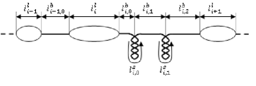
Figure 1: A typical configuration of a portion of the circular DNA model used in this study.

Let $L_{b},L_{s}$ and $L_{l}$ be the total length of bound, supercoil and loop segments respectively. The length of the DNA is given by $L_{b}+L_{s}+L_{l}=L$. The conservation of the linking number is imposed by the additional condition that an increase in the total loop length $L_{l}$ (reducing the linking number) is compensated by a proportional increase in the total supercoil length $L_{s}$ (recovering the linking number), and vice versa. Given the ground state $L_{b}=L$, $L_{s}=L_{l}=0$, this yields the constraint $L_{s}=\alpha L_{l}$. $\alpha$ is the proportionality constant and for simplicity we assume here $\alpha=1$, though the result is qualitatively the same for other values KOM2010 . In this model, as in the PS case, it is more convenient to work within a grand canonical ensemble, where the above constaint is relaxed to the equality of corresponding ensemble averages, i.e., $\langle L_{s}\rangle=\langle L_{l}\rangle$.

III Grand Canonical Treatment

For completeness we first outline the derivation in KOM09 for this case. To account for the two constraints above, the grand partition sum is constructed as a function of two fugacities $z$ and $\mu$ as

$$Q(z,\mu)=\sum_{L_{b},L_{s},L_{l}}Z(L_{b},L_{l}-L_{s})z^{L}\mu^{L_{l}-L_{s}},$$ (1)

where $Z(L_{b},L_{s}-L_{l})$ is the canonical partition sum. Note that for $\mu=1$, Eq. (1) is the grand canonical partition function of the Poland-Scheraga model extended to include all possible supercoil segment insertions. While this partition sum is different from that of the original PS model, it qualitatively yields the same phase diagram KOM09 .

The values of $z$ and $\mu$ are set by the conditions

$$L = \frac{\partial\log Q}{\partial\log z}\ \ (=L_{b}+L_{s}+L_{l}),$$ (2)

$$0 = \frac{\partial\log Q}{\partial\log\mu}\ \ (=L_{l}-L_{s}).$$ (3)

Assuming that there is at least one bounded base pair, the grand partition sum can be written as

$$Q(z,\mu) = \tilde{V}(z,\mu)+\tilde{V}(z,\mu)U(z\mu)\tilde{V}(z,\mu)+...$$ (4)

$$= \frac{\tilde{V}(z,\mu)}{1-\tilde{V}(z,\mu)U(z\mu)},$$ (5)

with

$$\tilde{V}(z,\mu) = \frac{V(z)}{1-V(z)W(z/\mu)},$$ (6)

$$V(z) = \sum_{n=1}^{\infty}\left(\omega z\right)^{n}=\frac{\omega z}{1-\omega z},$$ (7)

$$W(z/\mu) = \sum_{n=1}^{\infty}\left(\nu\frac{z}{\mu}\right)^{n}=\frac{\nu z}{\mu-\nu z},$$ (8)

$$U(z\mu) = \sum_{n=1}^{\infty}A\frac{\left(sz\mu\right)^{n}}{n^{c}}=A\Phi_{c}(sz\mu).$$ (9)

The functions $U,V$ and $W$ represent the grand partition sums for loops, bound segments and supercoils respectively. The polylog function $\Phi_{c}(q)$ is given by

$$\Phi_{c}(q)=\sum_{n=1}^{\infty}\frac{q^{n}}{n^{c}}.$$ (10)

It is an analytic function everywhere except for a branch cut at $q\in[1,\infty)$ Lewin1981 . It satisfies the relation

$$\frac{d}{dq}\Phi_{c}(q) = \frac{1}{q}\Phi_{c-1}(q)\ .$$ (11)

By inserting Eqs. (6-9) into (5), $Q(z,\mu)$ can be written as

$$Q(z,\mu)=\left[\left(\frac{1}{\omega z}-1\right)-\frac{\nu z}{\mu-\nu z}-A\Phi_{c}(sz\mu)\right]^{-1}.$$ (12)

From this explicit form the constraints given by Eqs.(2-3) are readily transformed into

$$\left(\frac{1}{\omega z}-1\right)-\frac{\nu z}{\mu-\nu z} = A\Phi_{c}(sz\mu),$$ (13)

$$\frac{\nu z}{(\mu-\nu z)^{2}} = \frac{A}{\mu}\Phi_{c-1}(sz\mu),$$ (14)

where $z$ and $\mu$ from here on refer to the corresponding values in the thermodynamic limit ($L\to\infty$) which is assumed in the derivation of Eq.(13). Denoting by $m_{b}$, $m_{s}$ and $m_{l}$ the average density of base pairs in bound segments, supercoils and loops, respectively, one finds that

$$m_{b} = -\frac{\partial\log z}{\partial\log\omega},$$ (15)

$$m_{s} = -\frac{\partial\log z}{\partial\log\nu},$$ (16)

$$m_{l} = -\frac{\partial\log z}{\partial\log s}.$$ (17)

It is more convenient to work with the transformed variables $x=sz\mu$ and $y=\nu z/\mu$. Physically $\left(x/s\right)$ is the fugacity associated with a unit increase in the total loop length, and $\left(y/\nu\right)$ is the similar fugacity of supercoils. Under this change of variables Eqs.(13, 14) become

$$\frac{\sqrt{s\nu}}{\omega\sqrt{xy}}-\frac{1}{1-y} = A\Phi_{c}(x),$$ (18)

$$\frac{y}{(1-y)^{2}} = A\Phi_{c-1}(x).$$ (19)

Considering $y$ as a function of $x$ through Eq.(19), let

$$G(x)\equiv\sqrt{\frac{xy}{s}}\left[A\Phi_{c}(x)+\frac{1}{1-y}\right],$$ (20)

so that Eq.(18) can be written as

$$G(x)=\nu^{1/2}\omega^{-1}=e^{\beta\left(E_{b}-\frac{1}{2}E_{s}\right)}\equiv H(T).$$ (21)

Note that $y$ and $G(x)$ are increasing functions of $x$ in the physically relevant regime $0\leq x\leq 1$. The lower bound $x=0$ is achieved at zero temperature since $\lim_{T\to 0}H(T)=0$, while the upper bound is unity since $\Phi_{c}(x)$ is a divergent sum for $x>1$. The presence of a thermodynamic phase transition then depends on whether $x(T_{c})=1$ is achieved for some finite temperature $T_{c}$. Two regimes emerge as shown in Fig.2:
(i) $c\leq 2$: $\lim_{x\to 1}\Phi_{c-1}(x)=\infty$, therefore Eqs.(18,19) have a solution in the interval $0\leq x<1$ at all temperatures,
(ii) $c>2$: Note that $\Phi_{\alpha}(1)=\sum_{n}1/n^{\alpha}=\zeta_{\alpha}$ is the Riemann Zeta function AS1964 . Then, as $x\to 1$, the RHS of Eqs.(18,19) remain finite since $\infty>\zeta_{c-1}>\zeta_{c}>1$. For suitable values of $A$ and $s$ (which guarantee $G(1)<1$), there exists a temperature $T_{c}$ such that $x(T\geq T_{c})=1$. The resulting nonanalyticity at $T_{c}$ translates into the singular behavior of other quantities like the density $m_{b}$ which underlies the melting transition. $T_{c}$ is given by

$$G\left(1\right)=\nu_{c}^{1/2}\omega_{c}^{-1}=e^{\frac{1}{T_{c}}\left(E_{b}-\frac{1}{2}E_{s}\right)}.$$ (22)

Below $T_{c}$, the system is fully defined by Eqs.(18, 19). Above $T_{c}$ one has

$$x=sz\mu=1\ ,$$ (23)

and an additional equation is necessary to impose the two constraints above. To this end, we follow Ref.KMP2002 and introduce a cutoff $M$ on the maximal loop size. In this reduced ensemble the partition function is analytic, thus Eqs.(13, 14) are valid at all temperatures. The limit $M\to\infty$ reveals precisely how these equations are modified above $T_{c}$, as discussed below.

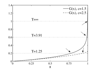
Figure 2: A plot of $G(x)$, as defined in (20), as function of $x$. The solid line corresponds to $c=1.5$ while the dashed line to $c=2.5$. The horizontal lines corresponds to different temperatures. The arrows point to the solutions of Eq.(18) which is equivalent to the thermodynamic limit. While for $c=1.5$ there exists a solution for all temperatures, for $c=2.5$ there is a solution only up to some finite temperature, in this case $\nu_{c}^{1/2}\omega_{c}^{-1}\approx 0.25$. The parameters which were used in this plot are $E_{b}=-3$, $E_{s}=-2$, $s=5$ and $A=0.1$.

III.1 Regularizing the Grand Canonical Ensemble

Introducing an upper cutoff $M$ on the allowed loop size, the loop partition sum $U(z\mu)$ is replaced by

$$U_{M}(z\mu)=A\sum_{n=1}^{M}\frac{(sz\mu)^{n}}{n^{c}}\equiv A\Phi_{c}^{M}(sz\mu),$$

where $\Phi_{c}^{M}(q)$ is the “loop-truncated” Polylog function, while the relation $\frac{d}{dq}\Phi_{c}^{M}(sq)=\frac{1}{q}\Phi_{c-1}^{M}(sq)$ still holds. The grand canonical partition sum is then

$$Q_{M}(z,\mu)=\frac{\tilde{V}(z,\mu)}{1-\tilde{V}(z,\mu)U_{M}(z\mu)},$$

and Eqs.(2,3) for the constraints can be written as

$$\left(\frac{1}{\omega z}-1\right)-\frac{\nu z}{\mu-\nu z} = A\Phi_{c}^{M}(sz\mu),$$ (24)

$$\frac{\nu z}{(\mu-\nu z)^{2}} = \frac{A}{\mu}\Phi_{c-1}^{M}(sz\mu).$$ (25)

These equations hold for all $T$, since $\Phi_{c}^{M}(x)$ is an analytic function. Our goal now is to analyze these equations in the limit $M\to\infty$ for temperatures above $T_{c}$. In this approach one should, in fact, consider the grand canonical ensemble with a finite but large average length of the DNA molecule $\left<L\right>$. One should then consider the limit $M,\left<L\right>\rightarrow\infty$ with $M\sim O(\left<L\right>)$. While considering finite $\left<L\right>$, Eq.(24) is no longer exact but has $O\left(\left<L\right>^{-1}\right)$ correction. However, this correction does not modify the analysis presented below as it vanishes in the limit $M\sim\left<L\right>\rightarrow\infty$. We therefore take $\left<L\right>=\infty$ and then $M\rightarrow\infty$.

Let $T_{c}^{M}$ be the temperature at which $sz\mu=1$ in this loop-truncated model, so that for $T>T_{c}^{M}$ we have $sz\mu=1+\epsilon(M,T)$ with $\epsilon>0$. Clearly, as $M\to\infty$, $T_{c}^{M}\to T_{c}$ and $\epsilon\to 0$ so that $sz\mu=1$ for all $T>T_{c}$. Then, for a given temperature $T>sup_{M}\left(T_{c}^{M}\right)$ we have

$$\frac{1}{\omega z}-\frac{\mu}{\mu-\nu z} = A\left(\Phi_{c}^{M}(1)+b(\epsilon)\right),$$ (26)

$$\frac{\nu z}{\left(\mu-\nu z\right)^{2}} = \frac{A}{\mu}\left(\Phi_{c-1}^{M}(1)+a(\epsilon)\right),$$ (27)

where

$$sz\mu=1+\epsilon,$$ (28)

and where $a(\epsilon)$ and $b(\epsilon)$ are cutoff-dependent corrections at least one of which is nonzero (otherwise the system is overdetermined). We continue by assuming that $M\epsilon\to\infty$ as $M\to\infty$, and checking that this assumption is self consistent. With this assumption the leading behavior of $a(\epsilon)$ and $b(\epsilon)$ is found as

$$a(\epsilon) = \sum_{n=1}^{M}\frac{(1+\epsilon)^{n}-1}{n^{c-1}}$$ (29)

$$\approx \int^{M}dx\frac{e^{\epsilon x}-1}{x^{c-1}}$$

$$\sim \frac{e^{\epsilon M}}{M^{c-1}}\left(\frac{1}{\epsilon}+O\left(\frac{1}{M}\right)\right),$$

and

$$b(\epsilon)=\sum_{n=1}^{M}\frac{(1+\epsilon)^{n}-1}{n^{c}}\sim a(\epsilon)/M.$$ (30)

Therefore, the only cutoff-independent choice is $a(0)=a_{0}$ and $b(0)=0$ for some constant $a_{0}$. Moreover, the asymptotic form of $\epsilon$ as a function of $M$ follows from Eq.(29) as

$$\epsilon(M,T) = (c-2)\frac{\log M}{M}+O\left(\frac{\log\log M}{M}\right),$$ (31)

demonstrating the self-consistency of the assumption above (see also EH2005 ). We conclude that while for $T<T_{c}$ Eqs.(13-14) hold, above $T_{c}$ they are replaced by

$$\frac{1}{\omega z}-\frac{\mu}{\mu-\nu z} = A\zeta_{c},$$ (32)

$$\frac{\nu z}{\left(\mu-\nu z\right)^{2}} = \frac{A}{\mu}\left(\zeta_{c-1}+a_{0}\right),$$ (33)

$$sz\mu = 1,$$ (34)

from which we can extract $a_{0}$

$$a_{0}=\frac{\nu}{As\left(\mu-\nu z\right)^{2}}-\zeta_{c-1}.$$ (35)

It measures the density of base pairs that reside within a macroscopic loop - or condensate - that appears above $T_{c}$. In the next section we discuss the order of the phase transition, where we take into account the condensate correction which was omitted in Ref. KOM09

III.2 Order of the Transition

We show below that the above phase transition is continuous and then investigate the nature of the singularity at $T_{c}$. Consider the fraction of base pairs in bound segments, i.e., $m_{b}=-\partial log(z)/\partial log(\omega)$. Defining

$$P\equiv Q^{-1}(z,\mu;\omega)=\frac{1}{\omega z}-\frac{\mu}{\mu-\nu z}-A\Phi_{c}(sz\mu),$$ (36)

and noting that $P(z,\mu;\omega)=0$ for the poles of the partition function, the smallest of which yields the thermodynamic limit, we find

$$0=\frac{dP}{d\omega}=\frac{\partial P}{\partial\omega}+\frac{\partial P}{\partial z}\frac{\partial z}{\partial\omega}+\frac{\partial P}{\partial\mu}\frac{\partial\mu}{\partial\omega}.$$ (37)

Rearranging and using Eq.(15)

$$m_{b}=\frac{\omega}{z}\frac{\partial P/\partial\omega}{\partial P/\partial z+\left(\partial P/\partial\mu\right)\left(\partial\mu/\partial z\right)}.$$ (38)

Evaluating the derivatives, making use of Eqs.(13,14, 23,36) we find that both below and above the critical temperature $m_{b}$ is given by

$$m_{b} = \left[1+\frac{2\omega\nu\mu z^{2}}{\left(\mu-\nu z\right)^{2}}\right]^{-1},$$ (39)

$$\equiv \left[1+\frac{2\omega y\sqrt{xy}}{\sqrt{s\nu}\left(1-y\right)^{2}}\right]^{-1},$$ (40)

Below $T_{c}$ this can be obtained by noting that Eq.(14) implies $\frac{\partial P}{\partial\mu}=0$. Equation (36) can then be used to calculate $\frac{\partial P}{\partial\omega}$ and $\frac{\partial P}{\partial z}$ and finally Eq.(14) is used again to eliminate the polylog function. Above $T_{c}$ Eq.(14) does not hold and is replaced by $sz\mu=1$. Equation (39) is then obtained by evaluating the partial derivatives appearing in Eq.(38). Equation (39) implies that the order parameter $m_{b}$ is continuous across the transition since $z$ and $\mu$ are continuous functions of the temperature. Thus the transition is continuous.

For a detailed analysis of the singularity it is convenient to express $m_{b}$ in terms of the $x,y$ variables. Let $\delta x$, $\delta y$, and $\delta m_{b}$ denote the deviation of $x$, $y$, and $m_{b}$, respectively, from their values at $T_{c}$ due to a slight change in temperature $t=T-T_{c}$. First we explore the relations among $t$, $\delta x$ and $\delta y$. Above the transition $x=1$ and hence $\delta x=0$. Thus $\Phi_{c}(x)$ in Eq.(18) becomes $\zeta_{c}$. As a result $y$ has a power series expansion above $T_{c}$ where to leading order $\delta y\propto t$. Hence for $t>0$, $\delta m_{b}=f(t)$ where $f$ is analytic near $t=0$. Below the transition one has to make use of the expansion of the polylog function

$$\Phi_{c-1}(1-\delta x)=\zeta_{c-1}+\zeta_{c-2}\delta x+...+\Gamma(c-2)\delta x^{c-2}+...$$ (41)

where $\Gamma(c-2)$ is the Gamma function and the last term is the leading singular term in the expansion. We proceed by separately considering two regimes of the parameter $c$.

• For $2<c<3$, the expansion (41) becomes $\Phi_{c-1}(1-\delta x)\approx\zeta_{c-1}+\Gamma(c-2)\delta x^{c-2}$ and therefore Eq.(19) yields

  $$\delta y\sim\delta x^{c-2},$$ (42)

  which implies $\delta x\ll\delta y$. Thus in the vicinity of the transition temperature Eqs.(18, 40) yield $\delta m_{b}\approx f(t)+\tilde{\alpha}\delta x$ where $f(t)$ is the same function as above the transition, and $\tilde{\alpha}$ is a constant. Using (42) and noting that $\delta y\propto t$ one finally obtains $\delta m_{b}=f(t)+\alpha t^{\frac{1}{c-2}}$ where $\alpha$ is a constant. Since $f(t)$ is analytic function, the $\left\lceil\frac{1}{c-2}\right\rceil$ derivative of $m_{b}$ is discontinuous and the transition is of order $\left\lceil\frac{c-1}{c-2}\right\rceil$ .
  

• For $c\geq 3$, the expansion of the polylog function is $\Phi_{c-1}(1-\delta x)\approx\zeta_{c-1}+\zeta_{c-2}\delta x$. Hence Eq.(19) yields $\delta y\propto\delta x$, which together with (18) implies $\delta x\propto\delta y\propto t$. Thus $\delta m_{b}\approx f(t)+\gamma t$ where $\gamma$ is a constant. This implies that the first derivative of $\delta m_{b}$ is discontinuous, and the transition is of second order.
  

In summary, the transition is characterized by the singular behavior of $\delta m_{b}$ below:

$$\delta m_{b}=\left\{\begin{array}[]{lcc}f(t)&&t>0\\ f(t)+\alpha t^{\eta}&&t>0\\ \end{array}\right.,$$ (43)

with

$$\eta=\left\{\begin{array}[]{ccr}\frac{1}{c-2}&&2<c<3\\ 1&&c\geq 3\\ \end{array}\right.,$$ (44)

where $f(t)$ can be expressed as a power series in $t$ for $t>0$. Since $m_{l}=m_{s}=(1-m_{b})/2$, a similar singular behavior is exhibited by these variables. Hence the denaturation transition of a circular DNA is second order for $c\geq 3$, third order for $2.5\leq c<3$, forth order for $\frac{7}{3}\leq c<2.5$, etc., approaching infinite order as $c\to 2$. No phase transition takes place for $c\leq 2$. In contrast, a DNA without helicity (as described by the original PS model) melts through a first order transition for $c>2$ and a second order transition for $1<c\leq 2$.

III.3 High Temperature Phase

The high-temperature phase of the PS model is composed of an all-encompassing macroscopic loop created at $T_{c}$ through a jump in the loop fraction to its maximum value $m_{l}=1$. Here, we not only have a smoother transition but also a qualitatively different denatured phase. For example, the loop fraction reaches its maximum value ($m_{l}=1/2$ within the present model) only as $T\to\infty$ and it continuously increases across and above $T_{c}$. At this point, one is tempted to ask what has changed qualitatively across the transition. In this section, we show that a macroscopic loop is again the distinguishing feature. However, instead of being an all-or-none phenomenon, the dominance of the macro-loop among the denatured base pairs grows steadily from $T_{c}$ on. Below we analyze the loop length distribution, $p_{M}(l)$, demonstrating that in addition to the power law behavior on microscopic scale, it exhibits a peak at lengths of order $M$ whose integrated weight is of order $1/M$. This peak represents the macroscopic loop which opens up above $T_{c}$. Note that the probability distribution functions for bound and supercoiled segment lengths are still exponential in the length $n$, since the corresponding Boltzmann weights are $(\omega z)^{n}$ and $y^{n}$, respectively.

The loop size distribution in the “loop-truncated” model is given by

$$p_{M}(l)=\frac{1}{\Phi_{c}^{M}(sz\mu)}\frac{(sz\mu)^{l}}{l^{c}}\Theta(M-l),$$ (45)

where $\Theta(x)$ is the Heaviside function. Differentiating with respect to $l$ and noting that $sz\mu=e^{\epsilon}$ we find that this distribution exhibits a minimum at

$$l^{*}=\frac{c}{\epsilon}=\frac{c}{c-2}\frac{M}{\log M},$$ (46)

where Eq.(31) has been used. The large $l$ distribution is peaked at $l=M$ with $p_{M}(M)\approx\zeta_{c}^{-1}e^{\epsilon M}/M^{c}\sim M^{-2}$. Thus the integrated weight of the peak is $O(1/M)$ up to logarithmic corrections. Since as discussed above $M\sim O(L)$, One expects $O(1)$ number of macroscopic loops to open up above $T_{c}$. In fact one can argue that entropy favors a single macroscopic loop EH2005 . To see this one can compare the probability of a state with only one macroscopic loop with that of configurations with two macroscopic loops: Assuming that there are $l_{con}\sim M$ base pairs within the condensed phase, the weight of configurations with single loop is

$$\Gamma_{1}\left(l_{con}\right)\approx L_{l}p_{M}\left(l_{con}\right)\sim O\left(L^{1-c}\right)(sz\mu)^{l_{con}}.$$

The weight of configurations with two macroscopic loops is

$$\Gamma_{2}\left(l_{con}\right) \approx \binom{L_{l}}{2}\sum_{n\sim M}p_{M}\left(n\right)p_{M}\left(l_{con}-n\right)$$

$$\sim O\left(L^{3-2c}\right)(sz\mu)^{l_{con}}.$$

As $c>2$, it follows that configurations with a single macroscopic loop dominates the ensemble in the limit $M\sim L\rightarrow\infty$.

The condensation phenomenon observed in this model is reminiscent of condensation in Bose-Einstein Gas and the zero-range process (ZRP) when the density of particles is above a critical value  EH2005 ; EMZ2006 . Figure 3 shows the loop size distribution for finite $M$ and $T>T_{c}$. A power-law decay with the exponent $c$ for $l\ll M$ and a peak for $l\lesssim M$ which is the precursor of the $\delta$-function representing the macroscopic loop are evident.

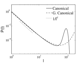
Figure 3: The loop size distribution $p(l)$ in the canonical (solid line) and the regularized grand-canonical (dashed line) ensembles. For small values of $l$ the critical phase can be identified (where $p(l)\sim l^{-c}$). For $l\sim L$ the canonical curve shows the “bump” around $l\approx\xi$ (see text) while the grand-canonical curve behaves in a somewhat different manner. The parameters which were used for this plot are $c=3.5$, $L=400$, $M=200$, $E_{b}=-3$, $E_{s}=-2$, $s=5$ and $A=0.1$ and $T=3$ ($T_{c}=1.167$)

IV Canonical Treatment

In order to justify the regularization procedure applied in the grand canonical ensemble we study the model within the canonical ensemble, namely with fixed $L$ and $L_{l}-L_{s}=0$. In addition this approach allows us to study the properties of the condensate and to further illuminate the mathematical structure underlying the phase transition. The canonical partition function can be obtained from the grand sum in Eq.(1) by means of Cauchy integration:

$$Z(L,L_{l}-L_{s})=\frac{1}{\left(2\pi i\right)^{2}}\oint_{C^{(\mu)}}d\mu\oint_{C^{(z)}}dz\frac{Q\left(z,\mu\right)}{z^{L+1}\mu^{L_{l}-L_{s}+1}},$$ (47)

where $C^{(\mu)}$ and $C^{(z)}$ are circular, counter-clockwise oriented contours which are centered at the origin and enclose no singularity of $Q(z,\mu)$ (Fig.4). Enforcing the linking number constraint, $L_{l}=L_{s}$, and using Eq.(12) yield

$$Z(L,0) = \frac{1}{\left(2\pi i\right)^{2}}\oint d\mu\oint dz\ I(z,\mu),$$ (48)

$$I(z,\mu) = \frac{\left[\frac{1}{\omega z}-1-\frac{\nu z}{\mu-\nu z}-A\Phi_{c}(sz\mu)\right]^{-1}}{z^{L+1}\mu}.$$ (49)

For $|\mu|$ sufficiently small so that $|sz\mu|<1$, let $z_{0}$ be the nontrivial pole of $I(z,\mu)$ in the $z$-plane, given by Eq.(13). Then, by Cauchy’s integral theorem, the integration contour $C^{(z)}$ can be replaced by $C_{p}^{(z)}+C_{bc}^{(z)}$ shown in Fig.4. Due to the factor $z^{-L}$ in (49) the dominant contribution comes from $C_{p}^{(z)}$ and we obtain

$$Z(L,0)\sim\frac{1}{2\pi i}\oint_{C^{(\mu)}}\frac{d\mu}{\mu}z_{0}(\mu)^{-L-1}.$$ (50)

We now evaluate the integral separately below and above the critical point. Below the transition, the integrand in Eq.(50) has a saddle point given by $\frac{dz_{0}}{d\mu}|_{\mu_{0}}=0$ and $|\mu_{0}|<1/s|z_{0}|$. The partition function can now be evaluated by first deforming $C^{(\mu)}$ into the contour $C_{s}^{(\mu)}$ which passes through this saddle point (Fig.4) and then approximating the integral by the contribution from the vicinity of $\mu_{0}$, i.e.,

$$Z(L,0)\sim e^{-L\log z_{0}(\mu_{0})}.$$ (51)

After differentiating Eq.(13) with respect to $\mu$ and setting $\frac{dz_{0}}{d\mu}=0$ we find Eq.(14) as the saddle-point condition. These two equations fix $z_{0}$ and $\mu_{0}$ and describe the system for $T<T_{c}$, as was found earlier in the grand-canonical framework. Note that the free energy is obtained from $z_{0}$ through Eq.(51).

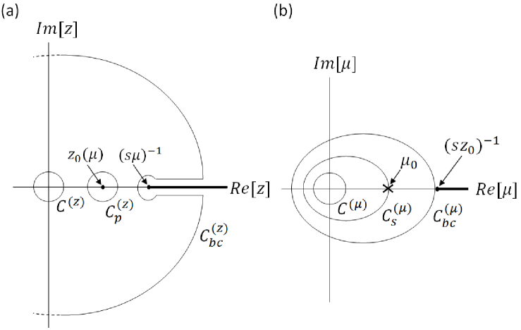
Figure 4: The integration procedure used for the canonical partition function: (a) In the $z$ plane, the contour $C^{(z)}$ which encircles the origin can be replaced by $C_{p}^{(z)}$ around the pole at $z_{0}$ and $C_{bc}^{(z)}$ which wraps the branch cut (thick line) and closes at infinity; (b) in the $\mu$ plane, the contour $C^{(\mu)}$ can be deformed to pass through a saddle point $\mu_{0}$ when it exits. Otherwise the dominant contribution comes from the vicinity of the branch point (see text).

Above the critical temperature, this procedure is not applicable, as the solution of $\frac{dz_{0}}{d\mu}=0$ for $\mu_{0}$ now lies on the branch cut. However, it is found that Eq.(51) holds, with $z_{0}$ and $\mu_{0}$ given now by Eqs.(13,23) rather than (13,14) as obtained within the grand canonical ensemble. This can be shown by evaluating the integral in Eq.(50) along another contour $C_{bc}^{(\mu)}$ shown in Fig.4 on which $|sz_{0}\mu|\lesssim 1$. After a change of variables $e^{-u}=sz_{0}\mu$, Eq.(50) transforms to

$$Z(L,0)\sim\oint\frac{du}{2\pi i}\ \alpha(u)\,e^{-L\log z_{0}(u)},$$ (52)

where $\alpha(u)=\frac{-1}{z_{0}}\left(1+\frac{d\log z_{0}}{du}\right)$ is a nonextensive correction to the free energy that can be neglected. The main contribution along the contour $C_{bc}^{(\mu)}$ is from the neighborhood of the branch cut where $|u|\ll 1$ with $\mbox{Re}[u]$ positive and as small as desired. We therefore express $\log\,z_{0}(u)$ in terms of the small parameter $u$ by using the implicit equation (13) and the nonanalytic expansion of $\Phi_{c}(1-u)$ given by Eq.(41), to obtain

$$\log z_{0}(u)\approx\sum_{n=0}^{\left\lfloor c-1\right\rfloor}b_{n}u^{n}+b_{c}u^{c-1}+...$$

where ${b_{n}}$ are temperature dependent coefficients with $b_{0}=\log z_{0}(0)$ and $b_{n}=\frac{1}{n!}\frac{d^{n}\log z_{0}}{du^{n}}|_{u=0}$. The coefficient of the linear term $b_{1}$ vanishes at $T_{c}$. This follows directly from Eqs.(13,14,23). It changes sign from $b_{1}>0$ below the transition, where $sz_{0}\mu_{0}<1$, to $b_{1}<0$ above it. Let $g(u)$ be the nonlinear part of the expansion $g(u)\approx\sum_{n=2}^{\left\lfloor c-1\right\rfloor}b_{n}u^{n}+b_{c}u^{c-1}$. Note that for $c<3$, $g(u)=b_{c}u^{c-1}$. One therefore has

$$Z(L,0)\sim e^{-L\log z_{0}(0)}\oint\frac{du}{2\pi i}\,e^{-L\left[b_{1}u+g(u)\right]}\ .$$ (53)

As $u$ is approximately imaginary in the region of interest, the integrand is oscillatory, yielding vanishing contribution at large $L$ except in the small region where $\mbox{Im}[u]\lesssim O\left(\frac{1}{L}\right)$. As a result one may expand the integrand in Eq.(53) as $e^{-L\left[b_{1}u+g(u)\right]}\approx e^{-b_{1}Lu}\left[1-Lg(u)\right]$. Moreover, the integration contour can be replaced by the right vertical tangent of $C_{bc}^{(\mu)}$ in Fig.4. Combining these observations we get

$$Z(L,0)\sim e^{-L\log z_{0}(0)}\int_{-i\infty}^{i\infty}du\,e^{-b_{1}Lu}\left[1-Lg(u)\right].$$ (54)

The analytic terms of the integrand do not contribute, since the integration yields a delta function $\delta\left(b_{1}L\right)$ or its derivatives EMZ2006 . Therefore, the partition function is determined solely by the nonanalytic term in $g(u)$ as:

$$Z(L,0) \sim e^{-L\log z_{0}(0)}b_{c}L\int_{-i\infty}^{i\infty}du\,e^{-b_{1}Lu}u^{c-1}$$ (55)

$$= e^{-L\log z_{0}(0)}\frac{\tilde{b}}{b_{1}^{c}L^{c-1}},$$

where $\tilde{b}\equiv b_{c}\frac{sin\left(\pi c\right)}{\pi}\Gamma(c)$ EMZ2006 . The free energy density is, of course, continuous across $T_{c}$ and above the critical temperature it is determined by Eqs.(13) and (23), as in the grand canonical treatment.

IV.1 High Temperature Phase

In this subsection we consider the loop size distribution $p(l)$ at temperatures above $T_{c}$. As in the grand canonical ensemble, a condensate phase composed of a macroscopic loop is found, although the details of the peak in $p(l)$ corresponding to this phase are different. The analysis follows the analysis carried out for the condensation transition in the zero-range process EMZ2006 . Here we just outline the main results.

Within the canonical ensemble the loop size distribution is given by

$$p(l)=A\frac{s^{l}}{l^{c}}\frac{Z(L-l,-l)}{Z(L,0)},$$ (56)

where $Z(L-l,-l)$ is given by

$$Z(L-l,-l) = \frac{1}{\left(2\pi i\right)^{2}}\oint_{C^{(\mu)}}d\mu\oint_{C^{(z)}}dz\frac{Q\left(z,\mu\right)}{z^{L+1-l}\mu^{1-l}}$$

$$\approx \frac{s^{-l}}{2\pi i}\oint_{C^{(\mu)}}d\mu\left(sz_{0}\mu\right)^{l}e^{-L\log z_{0}(\mu)}$$

$$\approx \frac{s^{-l}}{2\pi i}\oint_{C_{bc}^{(\mu)}}du\,e^{-L\left[\log z_{0}(u)+\phi u\right]},$$

with $\phi=l/L$ and $e^{-u}=sz_{0}\mu$. Expanding for small $u$ yields

$$p(l) \approx \frac{A}{l^{c}}\frac{I(l/L)}{I(0)},$$ (57)

$$I(\phi) \equiv \frac{1}{2\pi i}\int_{-i\infty}^{i\infty}du\,e^{-L\left[(b_{1}+\phi)u+g(u)\right]}.$$ (58)

For $T>T_{c}$, the function $I(\phi)$ develops a peak at $\phi\simeq-b_{1}\equiv\xi$. This is demonstrated separately for $2<c<3$ and $c>3$.

(a) For $2<c<3$, the leading-order term in $g(u)$ is the nonanalytic term $u^{c-1}$ and $I(\phi)$ can be written in the form

$$I(\phi)=L^{-1/(c-1)}V_{c}\left[L^{\frac{c-2}{c-1}}(\phi-\xi)\right].$$ (59)

The asymptotic behavior of the scaling function $V_{c}[q]$ are given by

$$V_{c}[q]\simeq\begin{cases}a|q|^{-c}&q\rightarrow-\infty\\ c_{1}q^{(3-c)/2(c-2)}e^{-c_{2}q^{(c-1)/(c-2)}}&q\rightarrow\infty,\end{cases}$$ (60)

where the constants $a$, $c_{1}$ and $c_{2}$ are given in Eqs.(81-83) of EMZ2006 . Equations(57-60) together with Eq.(55) yield after some algebra EMZ2006

$$p(l)\sim\begin{cases}\frac{l^{-c}}{(\xi-l/L)^{c}}&\xi L-l\gg O\left(L^{\frac{1}{c-1}}\right)\\ \frac{l^{-c}}{\left(\frac{l}{L}-\xi\right)^{\frac{c-3}{2(c-2)}}}e^{-c_{2}\left(\frac{l}{L}-\xi\right)^{\frac{c-1}{c-2}}}&\ \ l-\xi L\gg O\left(L^{\frac{1}{c-1}}\right).\end{cases}$$

In the intermediate regime where $|l-\xi L|\ll L^{\frac{1}{c-1}}$, $p(l)$ has the form

$$p(l)\sim L^{-c/(c-1)}V_{c}\left[\frac{l-L\xi}{L^{1/(c-1)}}\right].$$ (61)

Therefore $p(l)$ has a peak centered around $l\simeq\xi L$ with a power-law decay on the right and a stretched exponential decay on the left. Integrating $p(l)$ as given by (61) around $l\approx\xi L$ yields an order $1/L$ contribution implying the existence of a macroscopic loop.

(b) For $c>3$ the resulting behavior is summarized in Eqs.(100-101) of EMZ2006 and read

$$I(\phi)\simeq\begin{cases}\frac{a}{(\xi-\phi)^{c}L^{c-1}}&\xi-\phi\sim O(1)\\ \frac{1}{\sqrt{4\pi|b_{2}|L}}e^{L\frac{(\phi-\xi)^{2}}{4b_{2}}}&|\xi-\phi|\ll O\left(L^{-1/3}\right).\end{cases}$$

Note that $b_{2}<0$. Hence $p(l)$ is of the form

$$p(l)\sim\begin{cases}\frac{l^{-c}}{(\xi-l/L)^{c}}&\xi L-l\sim O(L)\\ \frac{(l/L)^{-c}}{L\sqrt{L}}e^{\frac{(l-\xi L)^{2}}{4b_{2}L}}&|\xi L-l|\ll O\left(L^{2/3}\right).\end{cases}$$

Therefore in this case the condensate bump has a Gaussian form with weight $O(1/L)$, as in the case $2<c<3$.

We conclude that the loop size distribution $p(l)$ is a power law (reminiscent of the critical phase) for $O(1)$ loops, superposed with a bump centered around $\xi L=|b_{1}|L$ as shown in Fig.3. The precise form of this condensate peak differs from the one found in the grand-canonical analysis, although both ensembles yield the same phase diagram in the large $L$ limit. This result is very similar to what is found in the context of ZRP, however it is not exactly the same. Within the ZRP, above the critical density any further increase in the density is absorbed by the condensate. Here, on the other hand, the total length of the loops in the critical phase changes with temperature above $T_{c}$. In particular, it is finite at $T_{c}$ and approaches zero at $T\rightarrow\infty$. Since the loop size distribution in the critical phase is fixed above the critical temperature, it implies that the number of loops in the critical phase varies with $T$.

V Conclusions

We analyzed the denaturation transition of circular DNA chains, assuming that opening denatured loops induces formation of supercoils. As in the case of non-circular DNA the thermodynamic behavior of the model is found to be determined by the loop entropy parameter $c$. We find that for $c\leq 2$ the model exhibits no transition while for $c>2$ the transition is continuous, of order $\left\lceil\frac{c-1}{c-2}\right\rceil$. Thus for $c\geq 3$ the transition is second order, while for $2<c<3$ (which includes the physical value of $c\approx 2.12$) it is of higher order reaching $\infty$-order as $c\to 2$.

In addition, the nature of the denaturated phase is rather different from that of the non-circular DNA. Here a macroscopic loop (condensate) is formed above $T_{c}$ whose length increases continuously as the temperature is increased. This is different from the denaturated phase in the non-circular case, where the two strands are fully separated at all temperatures above $T_{c}$. This is reminiscent of Bose-Einstein condensation and to similar real space condensation encountered in models such as the ZRP EH2005 ; EMZ2006 . Furthermore, the difference observed in the condensate peaks of canonical and grand-canonical ensembles (for finite $L$) has the same mathematical structure as in the ZRP.

A different mechanism for absorbing the extra linking number produced by opening of loops in circular DNA has been considered previously  RB2002 ; GOY2004 . In this mechanism the extra linking number is compensated by overtwist of remaining bound segments of the molecule at the cost of an elastic energy. This mechanism also yields smoothening of the denaturation transition as obtained in the present paper. It would be of interest to consider the denaturation transition in the case where both overtwist and supercoils are present.

Finally, our results apply to a homogeneous polymer where there is a single binding energy. It is well known that introducing disorder also smoothens the first-order transition in the PS model CY2007 . The influence of sequence inhomogeneity on the present melting transition which is already smoothened by topological constraints is an open question.

We thank O. Cohen, M.R. Evans, O. Hirschberg, S.N. Majumdar and E. Orlandini for helpful discussions. This work was supported by the Israel Science Foundation (ISF) and the Turkish Technological and Scientific Research Council (TUBITAK) through the grant TBAG-110T618.

References

- (1) D. Dixon, R. Simpson-White, and L. Dixon, J. Mar. Biol. Assoc. UK 72, 519 (1992).
- (2) D. Hickey and G. Singer, Genome biology 5, 117 (2004).
- (3) R. M. Wartell and A. S. Benight, Physics Reports 126, 67 (1985).
- (4) H. Hiasa and K. Marians, Journal of Biological Chemistry 269, 32655 (1994).
- (5) H. Hiasa and K. Marians, Journal of Biological Chemistry 271, 21529 (1996).
- (6) E. Carlon and T. Heim, Physica A: Statistical Mechanics and its Applications 362, 433 (2006).
- (7) M. Peyrard and A. R. Bishop, Phys. Rev. Lett. 62, 2755 (1989).
- (8) M. E. Fisher, J. Chem. Phys. 45, 1469 (1966).
- (9) D. Poland and H. A. Scheraga, J. Chem. Phys. 45, 1456 (1966).
- (10) T. Dauxois, M. Peyrard, and A. R. Bishop, Phys. Rev. E 47, 684 (1993).
- (11) Y. Kafri, D. Mukamel, and L. Peliti, Phys. Rev. Lett. 85, 4988 (2000).
- (12) R. Wartell and E. Montroll, Adv. Chem. Phys. 22, 129 (1972).
- (13) C. J. Benham, J. Chem. Phys. 72, 3633 (1980).
- (14) C. J. Benham, Journal of Molecular Biology 225, 835 (1992).
- (15) C. Bouchiat and M. Mezard, The European Physical Journal E: Soft Matter and Biological Physics 2, 377 (2000).
- (16) J. Palmeri, M. Manghi, and N. Destainville, Phys. Rev. Lett. 99, 088103 (2007).
- (17) J. F. Marko and E. D. Siggia, Macromolecules 27, 981 (1994).
- (18) R. A. Neher and U. Gerland, Phys. Rev. E 73, 030902 (2006).
- (19) Y. Kafri, D. Mukamel, and L. Peliti, Euro. Phys. J. B 27, 135 (2002).
- (20) E. Carlon, E. Orlandini, and A. L. Stella, Phys. Rev. Lett. 88, 198101 (2002).
- (21) R. Blake et al., Bioinformatics 15(5), 370 (1999).
- (22) J. Rudnick and R. Bruinsma, Phys. Rev. E. 65, 030902(R) (2002).
- (23) T. Garel, H. Orland, and E. Yeramian, Arxiv preprint q-bio/0407036 (2004).
- (24) A. Kabakçıoğlu, E. Orlandini, and D. Mukamel, Phys Rev E. 80, 010903(R) (2009).
- (25) A. Kabakçıoğlu, E. Orlandini, and D. Mukamel, Physica A: Statistical Mechanics and its Applications 389, 3002 (2010).
- (26) M. Sayar, B. Avşaroğlu, and A. Kabakçıoğlu, Physical Review E 81, 041916 (2010).
- (27) L. Yan and H. Iwasaki, Japanese Journal of Applied Physics 41, 7556 (2002).
- (28) B. Duplantier, Phys. Rev. Lett. 57, 941 (1986).
- (29) L. Lewin, Polylogarithms and Associated Functions (North-Holland Publishing Co., New York, 1981).
- (30) M. Abramowitz and I. Stegun, Handbook of Mathematical Functions, Fifth ed. (Dover, New York, 1964).
- (31) M. Evans and T. Hanney, Journal of Physics A: Mathematical and General 38, R195 (2005).
- (32) M. R. Evans, S. N. Majumdar, and R. K. P. Zia, J. Stat. Phys. 123(2), 357 (2006).
- (33) B. Coluzzi and E. Yeramian, The European Physical Journal B - Condensed Matter and Complex Systems 56, 349 (2007).