Direct computation of contagion triggering probabilities for generalized and bipartite random networks

Abstract

We derive a general expression for the probability of global spreading starting from a single infected seed for contagion processes acting on generalized, correlated random networks. We employ a simple probabilistic argument that encodes the spreading mechanism in an intuitive, physical fashion. We use our approach to directly and systematically obtain triggering probabilities for contagion processes acting on a collection of random network families including bipartite random networks. We find the contagion condition, the location of the phase transition into an endemic state, from an expansion about the disease-free state.

I Introduction

Spreading is a pervasive dynamic phenomenon, ranging in form from simple physical diffusion to the complexities of socio-cultural dispersion and interaction of ideas and beliefs Richerson and Boyd (2005); Chmiel et al. (2011); Romero et al. (2011); Rozin and Royzman (2001); Leskovec et al. (2009); Berger and Le Mens (2009); Banerjee (1992); Barsade (2002); Bikhchandani et al. (1992); Rogers (1995); Sieczka et al. (2011). Successful spreading in systems may manifest as an expanding front, such as in the spread of disease through medieval Europe Cliff et al. (1981), or through inherent or revealed networks, such as in pandemics in the modern era of global travel Colizza et al. (2007). Here, we focus on spreading processes operating on generalized random networks, which have proven over the last decade to be illustrative of spreading on real networks and at the same time to be analytically tractable Newman et al. (2001); Boguñá and Ángeles Serrano (2005); Meyers et al. (2006); Gleeson and Cahalane (2007); Gleeson (2008); Gleeson et al. (2010); Watts (2002); Hackett et al. (2011); Ikeda et al. (2010); Romero et al. (2011); Munz et al. (2009); Watts and Dodds (2009).

In contributing to the wealth of already known results for contagion on random networks, we make two main advances here. First, we obtain, in the most general terms possible, an expression for the probability of global spreading from a single seed for a broad range of contagion processes acting on generalized, correlated random networks. By global spreading we mean a non-zero fraction of nodes in an infinite network are eventually infected. Second, we use an argument that is physically motivated and direct. Existing approaches rely on a range of mathematical techniques, such as probability generating functions Wilf (2006); Newman et al. (2001); Newman (2003), which, while being entirely successful in determining spreading probabilities and higher moments of cascade size distribution, obscure the underlying physical mechanisms.

The present paper is a companion to our earlier work where we derived a general condition for the possibility (rather than probability) of global spreading for single-seed contagion processes acting on random networks Dodds et al. (2011). We used specific results from both works in a separate investigation of exactly solvable network spreading models Payne et al. (2011). As we show below, our expression for the probability of spreading naturally allows us to recover our expression for the possibility of spreading, and this is a purely mathematical exercise. Our key contribution is the direct derivation of triggering probabilities via physical arguments, as illustrated in Fig. 1.

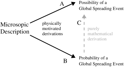
Figure 1: Physical and mathematical explanations of two fundamental aspects of broad classes of contagion processes acting on generalized random networks. In the present paper, we provide a physical approach to determining the probability of spreading from a single seed (derivation B). We use mathematical arguments to arrive again at the binary contagion condition (derivation C), which we obtained in a previous work Dodds et al. (2011) using a direct physical explanation (derivation A).

We structure our paper as follows. In Sec. II, we define the broadest class of correlated random networks allowing for directed and undirected edges and arbitrary node and edge properties. In Sec. III, we define the general class of contagion processes that our treatment can encompass. In Sec. IV, we compute the probability that seeding a node of a given type generates a global spreading event. For completeness, in Sec. V, we derive the contagion condition (location of the endemic phase transition) result found in Dodds et al. (2011), and we show how non-physical expressions may arise through this mathematical route. We use our formalism for six interrelated random network families with general contagion processes acting on them in Sec. VI.1. In Secs. VI.2 and VI.3, we show how our approach readily applies to random bipartite networks, and we offer some concluding remarks in Sec. VII.

II Generalized random networks

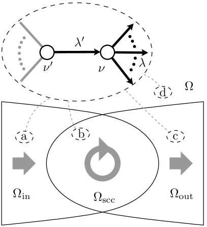
Figure 2: Schematic showing the configuration of the potential triggering node subnetwork using the present work’s formalism for generalized random networks described in Sec. II, and the basic form of a random network with directed edges and a giant component. The ellipses labelled a–d show four possible locations of the subnetwork in the overall network $\Omega$. Global spreading events can be successfully generated only if the subnetwork is part of the giant in-component $\Omega_{\rm in}$, either within or outside of the giant strongly connected component $\Omega_{\rm scc}$ (ellipses a and b). No spreading is possible if the subnetwork is instead part of the giant out-component outside of the strongly connected component ($\Omega_{\rm out}/\Omega_{\rm scc}$, ellipse c) or outside of all three giant components (ellipse d).

Our theoretical treatment builds on a formalism we introduce here for representing generalized random networks, an expansion of what we used in our connected, earlier work Dodds et al. (2011). Our theory applies to large random networks with bounded degrees (such as the configuration model), since these graphs are all locally tree-like and can be approximated by multitype branching processes. Generalized random networks may contain a combination of directed and undirected edges, so they are in general nonsimple graphs.

We depict the essential features of a random network with possibly directed edges in Fig. 2, noting that our analytic treatment will also cover more specialized random networks, such as those induced by bipartite graphs, or networks with multipartite structure (see Sec. VI.2). The most basic elements of networks are nodes and edges, and here we allow the following features encoded in two types of labels:

• Node type, $\nu\in\mathcal{N}$: arbitrary node characteristics such as node age, susceptibility to a given disease or message, etc. The node type implicitly includes information about its degree, which we explain below.

• Edge type, $\lambda\in\Lambda$: arbitrary edge characteristics such as age, strength, conductance, etc. Since edges may be directed, edge type includes whether an edge is directed or not and its orientation if so. We thus use the notation $\bar{\lambda}$ to indicate the edge’s type when considered as travelling in the disallowed direction. (There is no need to distinguish $\lambda$ or $\bar{\lambda}$ for undirected edges.) In other words, if there is a directed edge of type $\lambda$ from node $u$ to node $v$, we say there its type is $\bar{\lambda}$ when viewing $v$ as the source and $u$ as the target.

We take $\mathcal{N}$ and $\Lambda$ to be discrete. We denote the entire network by $\Omega$, and the set of edge types incident to a node of type $\nu$ by $\Lambda_{\nu}$.

We define degree as the number of edges of a certain type emanating from a node. In simple networks, we let $k(\nu,\lambda)$ denote the number of edges of type $\lambda$ emanating from a node of type $\nu$. In more general networks we let the multi-index $\vec{k}(\nu,\lambda)=\left[k_{\rm u}(\nu,\lambda),k_{\rm i}(\nu,\lambda),k_{\rm o}(\nu,\lambda)\right]$ denote the number of undirected, inward, and outward edges of type $\lambda$ belonging to a node of type $\nu$.

The ‘total degree’ of a node of type $\nu$ is then $\vec{k}(\nu)=\sum_{\lambda\in\Lambda_{\nu}}\vec{k}(\nu,\lambda)$, and we define the effective degree, a scalar important for spreading mechanisms, as $k^{(\rm eff)}(\nu,\lambda)=k_{\rm o}(\nu,\lambda)+k_{\rm u}(\nu,\lambda)$. We also introduce a directedness indicator function $d(\lambda)$ which equals one if edges of type $\lambda$ are directed and zero if not.

To characterize a random network with arbitrary node-edge-node correlations, we need to specify a number of interrelated probabilities, and these must further satisfy certain restrictions and detailed balance equations Boguñá and Ángeles Serrano (2005). First, we have the node and edge distributions $\mathbf{Pr}(\nu)$ and $\mathbf{Pr}(\lambda)$. Note that we immediately have the restriction $\mathbf{Pr}(\lambda)=\mathbf{Pr}(\bar{\lambda})$. Also, these induce the usual degree distributions via

$$\mathbf{Pr}(\vec{k})=\sum_{\nu\in\mathcal{N}}\mathbf{Pr}(\nu)\delta_{\vec{k},\vec{k}(\nu)}$$

where $\delta$ is the Kronecker delta.

Next we need $\mathbf{Pr}(\nu\lambda)$, defined as the probability that, in randomly choosing an edge and traversing it (in the allowed direction if directed or a random direction if undirected), we find it is of type $\lambda$ and that we are travelling away from a node of type $\nu$.

Finally, we encode correlations via the transition probability $\mathbf{Pr}(\nu|\nu^{\prime}\lambda^{\prime})$ which is the probability that we reach a type $\nu$ node, given that we are following a type $\lambda^{\prime}$ edge away from a type $\nu^{\prime}$ node. This includes the usual degree-degree transition probabilities (see Sec. VI.1 and Payne et al. (2011) for notation):

$$P^{(\rm\rm i)}(\vec{k}^{\prime\prime}|\vec{k}^{\prime}) =\sum_{\nu,\nu^{\prime}\in\mathcal{N}}\sum_{\lambda\in\Lambda_{\nu^{\prime}}}\mathbf{Pr}(\nu|\nu^{\prime}\lambda^{\prime})d(\lambda^{\prime})$$ (1)

$$\qquad\times\delta_{\vec{k}^{\prime},\vec{k}(\nu^{\prime})}\delta_{\vec{k}^{\prime\prime},\vec{k}(\nu)},$$

$$P^{(\rm\rm u)}(\vec{k}^{\prime\prime}|\vec{k}^{\prime}) =\sum_{\nu,\nu^{\prime}\in\mathcal{N}}\sum_{\lambda\in\Lambda_{\nu^{\prime}}}\mathbf{Pr}(\nu|\nu^{\prime}\lambda^{\prime})[1-d(\lambda^{\prime})]$$

$$\qquad\times\delta_{\vec{k}^{\prime},\vec{k}(\nu^{\prime})}\delta_{\vec{k}^{\prime\prime},\vec{k}(\nu)}.$$

We are now forced to connect and constrain the probabilities $\mathbf{Pr}(\nu\lambda)$ and $\mathbf{Pr}(\nu|\nu^{\prime}\lambda^{\prime})$ according to a detailed balance constraint. Consider $\mathbf{Pr}(\nu^{\prime}\lambda^{\prime}\nu)$ defined as the probability that a randomly selected edge is of type $\lambda^{\prime}$ and runs from a type $\nu^{\prime}$ node to a type $\nu$ node (corresponding to the subnetwork in Fig. 2). Then,

$$\mathbf{Pr}(\nu^{\prime}\lambda^{\prime}\nu)=\mathbf{Pr}(\nu|\nu^{\prime}\lambda^{\prime})\mathbf{Pr}(\nu^{\prime}\lambda^{\prime}).$$

Now, if we traversed the edge in the disallowed direction, it would “connect” a type $\nu$ node to a type $\nu^{\prime}$ node. Then we must also have $\mathbf{Pr}(\nu^{\prime}\lambda^{\prime}\nu)=\mathbf{Pr}(\nu\bar{\lambda^{\prime}}\nu^{\prime})$. We therefore arrive at the detailed balance condition:

$$\underbrace{\mathbf{Pr}(\nu|\nu^{\prime}\lambda^{\prime})\mathbf{Pr}(\nu^{\prime}\lambda^{\prime})}_{\mathbf{Pr}(\nu^{\prime}\lambda^{\prime}\nu)}=\underbrace{\mathbf{Pr}(\nu^{\prime}|\nu\bar{\lambda^{\prime}})\mathbf{Pr}(\nu\bar{\lambda^{\prime}})}_{\mathbf{Pr}(\nu\bar{\lambda^{\prime}}\nu^{\prime})}.$$ (2)

Note that the detailed balance condition, Eq. (2), is more general for typed random networks than the detailed balance conditions in terms of the degree distributions $\mathbf{Pr}(\vec{k},\vec{k}^{\prime})$ and $\mathbf{Pr}(\vec{k})$ found by Boguñá and Ángeles Serrano (2005). If the types of the nodes are their degrees and the edge types are $\Lambda=\{\rm undirected,incoming,outgoing\}$, then Eq. (2) reduces to the well-known detailed balance conditions given in Boguñá and Ángeles Serrano (2005) and Payne et al. (2011), which can all be written as

$$\underbrace{P^{(\lambda)}(k|k^{\prime})\frac{k_{\lambda}^{\prime}\mathbf{Pr}(k^{\prime})}{\langle k_{\lambda}\rangle}}_{P^{(\lambda)}(k,k^{\prime})}=\underbrace{P^{(\bar{\lambda})}(k^{\prime}|k)\frac{k_{\bar{\lambda}}\mathbf{Pr}(k)}{\langle k_{\lambda}\rangle}}_{P^{(\bar{\lambda})}(k^{\prime},k)}.$$ (3)

In networks where there are multiple types of directed or undirected edges, the detailed balance equations given in Boguñá and Ángeles Serrano (2005); Payne et al. (2011), which have the form of Eq. (3), are not necessarily valid. This is because not all edges or degree-$k$ nodes are equivalent. Using Eq. (2), we can show that the symmetry of the degree distributions is conserved, $\mathbf{Pr}(k,k^{\prime})=\mathbf{Pr}(k^{\prime},k)$.

$$\mathbf{Pr}(k^{\prime\prime},k^{\prime})=\sum_{\nu,\nu^{\prime}\in\mathcal{N}}\sum_{\lambda\in\Lambda_{\nu}}\mathbf{Pr}(\nu^{\prime}\lambda\nu)\delta_{k^{\prime},k(\nu^{\prime})}\delta_{k^{\prime\prime},k(\nu)}$$

In considering contagion processes, we recall the well-known typical macroscopic ‘bow-tie’ form of random networks with directed edges Newman et al. (2001); Broder et al. (2000); Boguñá and Ángeles Serrano (2005), given that a giant component is present. As shown in Fig. 2, there are three giant components of functional importance: (1) the giant strongly connected component, $\Omega_{\rm scc}$, within which any pair of nodes can be connected via a path of directed and/or undirected edges, traversing the directed ones; (2) the giant in-component $\Omega_{\rm in}$, the set of all nodes from which paths lead to $\Omega_{\rm scc}$ (n.b., $\Omega_{\rm scc}\subset\Omega_{\rm in}$); and (3) the giant out-component $\Omega_{\rm out}$, the set of all nodes which can be reached along directed paths starting from a node in $\Omega_{\rm in}$ (n.b., $\Omega_{\rm scc}\subset\Omega_{\rm out}$). By definition, we have that $\Omega_{\rm scc}=\Omega_{\rm in}\cap\Omega_{\rm out}$. Any global spreading event must begin from a seed in the giant in-component, and can at most spread to the giant out-component $\Omega_{\rm out}$.

III Generalized contagion process

We consider contagion processes where the probability of a node’s infection may depend in any fashion on the current states of its neighbors, potentially resembling phenomena ranging from the spread of infectious diseases to socially-transmitted behaviors Schelling (1973); Granovetter (1978); Murray (2002); Watts (2002). Since we are interested in the probability of spreading, we can capitalize on the fact that random networks are locally pure branching structures. We therefore need to know only what the probability of infection is for a type $\nu$ node given a single neighbor of type $\nu^{\prime}$ is infected, whose influence is felt along a type $\lambda^{\prime}$ edge. We write this probability as $B_{\nu^{\prime}\lambda^{\prime}\nu}$. Time is removed from this quantity, as we need to know only the probability of eventual infection. Disease spreading models with recovery Murray (2002); Dodds et al. (2011) are included, as are threshold models inspired by social contagion Granovetter (1978); Watts (2002).

IV Triggering probabilities

Network:	Edge Triggering Probability:	Node Triggering Probability, $Q$:
I. Undirected, Uncorrelated	$\displaystyle Q_{\ast\ast}=\sum_{k_{\rm u}}P^{(\rm\rm u)}(k_{\rm u}\,|\,\ast)B_{\ast\ast k_{\rm u}}\left[1-(1-Q_{\ast\ast})^{k_{\rm u}-1}\right]$	$\displaystyle\sum_{k_{\rm u}}\mathbf{Pr}(k_{\rm u})\left[1-(1-Q_{\ast\ast})^{k_{\rm u}}\right]$
II. Directed, Uncorrelated	$\displaystyle Q_{\ast\ast}=\sum_{k_{\rm i},k_{\rm o}}P^{(\rm\rm u)}(k_{\rm i},k_{\rm o}|\,\ast)B_{\ast\ast k_{\rm i}}\left[1-(1-Q_{\ast\ast})^{k_{\rm o}}\right]$	$\displaystyle\sum_{k_{\rm i},k_{\rm o}}\mathbf{Pr}(k_{\rm i},k_{\rm o})\left[1-(1-Q_{\ast\ast})^{k_{\rm o}}\right]$
III. Mixed Directed and Undirected, Uncorrelated	$\displaystyle Q_{\ast u}=\sum_{\vec{k}}P^{(\rm\rm u)}(\vec{k}|\,\ast)B_{\ast\ast\vec{k}}\left[1-(1-Q_{\ast u})^{k_{\rm u}-1}(1-Q_{\ast o})^{k_{\rm o}}\right]$ $\displaystyle Q_{\ast o}=\sum_{\vec{k}}P^{(\rm\rm i)}(\vec{k}|\,\ast)B_{\ast\ast\vec{k}}\left[1-(1-Q_{\ast u})^{k_{\rm u}}(1-Q_{\ast o})^{k_{\rm o}}\right]$	$\displaystyle\sum_{\vec{k}}\mathbf{Pr}(\vec{k})\left[1-(1-Q_{\ast u})^{k_{\rm u}}(1-Q_{\ast o})^{k_{\rm o}}\right]$
IV. Undirected, Correlated	$\displaystyle Q_{k_{\rm u}^{\prime}\ast}=\sum_{k_{\rm u}}P^{(\rm\rm u)}(k_{\rm u}\,|\,k_{\rm u}^{\prime})B_{\ast\ast k_{\rm u}}\left[1-(1-Q_{k_{\rm u}\ast})^{k_{\rm u}-1}\right]$	$\displaystyle\sum_{k_{\rm u}}\mathbf{Pr}(k_{\rm u})\left[1-(1-Q_{k_{\rm u}\ast})^{k_{\rm u}}\right]$
V. Directed, Correlated	$\displaystyle Q_{k_{\rm i}^{\prime}k_{\rm o}^{\prime},\ast}=\sum_{k_{\rm i},k_{\rm o}}P^{(\rm\rm u)}(k_{\rm i},k_{\rm o}|\,k_{\rm i}^{\prime},k_{\rm o}^{\prime})B_{\ast\ast k_{\rm i}}\left[1-(1-Q_{k_{\rm i}k_{\rm o},\ast})^{k_{\rm o}}\right]$	$\displaystyle\sum_{k_{\rm i},k_{\rm o}}\mathbf{Pr}(k_{\rm i},k_{\rm o})\left[1-(1-Q_{k_{\rm i}k_{\rm o},\ast})^{k_{\rm o}}\right]$
VI. Mixed Directed and Undirected, Correlated	$\displaystyle Q_{\vec{k}^{\prime}u}=\sum_{\vec{k}}P^{(\rm\rm u)}(\vec{k}|\,\vec{k}^{\prime})B_{\ast\ast\vec{k}}\left[1-(1-Q_{\vec{k}u})^{k_{\rm u}-1}(1-Q_{\vec{k}o})^{k_{\rm o}}\right]$ $\displaystyle Q_{\vec{k}^{\prime}o}=\sum_{\vec{k}}P^{(\rm\rm i)}(\vec{k}|\,\vec{k}^{\prime})B_{\ast\ast\vec{k}}\left[1-(1-Q_{\vec{k}u})^{k_{\rm u}}(1-Q_{\vec{k}o})^{k_{\rm o}}\right]$	$\displaystyle\sum_{\vec{k}}\mathbf{Pr}(\vec{k})\left[1-(1-Q_{\vec{k}u})^{k_{\rm u}}(1-Q_{\vec{k}o})^{k_{\rm o}}\right]$

Table 1: For the six classes of random networks described in Sec. VI.1, the probability of triggering a global spreading events due to (1) an infected edge, and (2) an infected, randomly chosen single seed (see Eqs. 4 and 6). We indicate by the symbol $\ast$ when no node or edge type is relevant.

We define $Q_{\nu\lambda}$ to be the probability that seeding a type $\nu$ node generates a global spreading event along an edge of type $\lambda$. Due to the Markovian nature of random networks, this probability must satisfy a nonlinear recursion relation:

$$Q_{\nu^{\prime}\lambda^{\prime}} =\sum_{\nu\in\mathcal{N}}\mathbf{Pr}(\nu|\nu^{\prime}\lambda^{\prime})B_{\nu^{\prime}\lambda^{\prime}\nu}$$ (4)

$$\;\;\;\times\left[1-\prod_{\lambda\in\Lambda_{\nu}}\left(1-Q_{\nu\lambda}\right)^{k^{(\rm eff)}(\nu,\lambda)-\delta_{\lambda,\bar{\lambda^{\prime}}}}\right],$$

an expression which involves the following three elements. First, we have $\mathbf{Pr}(\nu|\nu^{\prime}\lambda^{\prime})$ which is the probability of transitioning to a node of type $\nu$. The second term $B_{\nu^{\prime}\lambda^{\prime}\nu}$ is the probability of successful infection. The last term contains the recursive structure. At least one of the edges leading away from the type $\nu$ node must generate a global spreading event (note that we avoid double counting the incident edge of type $\bar{\lambda^{\prime}}$ with the indicator in the exponent). The probability this happens is the complement of the probability that none succeed, $\prod_{\lambda\in\Lambda_{\nu}}\left(1-Q_{\nu\lambda}\right)^{k^{(\rm eff)}(\nu,\lambda)-\delta_{\lambda,\bar{\lambda^{\prime}}}}.$ Eq. (4) will rarely be analytically tractable (but see Payne et al. (2011) for an exactly solved simple model), and will usually be solved numerically by iteration.

The probability that an infected type $\nu$ node seeds a global spreading event follows as

$$Q_{\nu}=1-\prod_{\lambda\in\Lambda_{\nu}}(1-Q_{\nu\lambda})^{k^{(\rm eff)}(\nu,\lambda)},$$ (5)

where again success is defined in terms of not failing. Finally, the probability that the sole infection of a randomly chosen node leads to a global spreading event is

$$Q=\sum_{\nu^{\prime}\in\mathcal{N}}\mathbf{Pr}(\nu^{\prime})Q_{\nu^{\prime}}$$ (6)

The effects of weighted triggering schemes—where the initial node is chosen according to its degree in some fashion—can be easily examined by replacing $\mathbf{Pr}(\nu^{\prime})$ with the appropriate distribution.

V Connection between triggering probabilities and the contagion condition

We show how our general expression for triggering probabilities reduces to the general cascade condition we described in Dodds et al. (2011). The calculation involved makes an important analytic connection but is necessarily largely mathematical in nature, as represented in Fig. 2.

The cascade condition is a binary expression of possibility; when the condition is met, global spreading events initiated by single seeds are possible, and otherwise they are impossible. Starting from Eq. (4), we determine the cascade condition by examining under what circumstances the triggering probability $Q_{\nu\lambda}\rightarrow 0^{+}$. In this limit, the product in Eq. (4), $\prod_{\lambda\in\Lambda_{\nu}}\left(1-Q_{\nu\lambda}\right)^{k^{(\rm eff)}(\nu,\lambda)-\delta_{\lambda,\bar{\lambda^{\prime}}}}.$ can be approximated as $1-\sum_{\lambda\in\Lambda_{\nu}}\left(k^{(\rm eff)}(\nu,\lambda)-\delta_{\lambda,\bar{\lambda^{\prime}}}\right)Q_{\nu\lambda},$ to first order. Neglecting higher order terms, Eq. (4) reduces to

$$Q_{\nu^{\prime}\lambda^{\prime}} \simeq\sum_{\nu\in\mathcal{N}}\mathbf{Pr}(\nu|\nu^{\prime}\lambda^{\prime})B_{\nu|\lambda^{\prime}\nu^{\prime}}$$ (7)

$$\quad\times\sum_{\lambda\in\Lambda_{\nu}}\left(k^{(\rm eff)}(\nu,\lambda)-\delta_{\lambda,\bar{\lambda^{\prime}}}\right)Q_{\nu\lambda}.$$

We introduce the notation from Dodds et al. (2011), where $\alpha=(\nu,\lambda)$ and $\alpha^{\prime}=(\nu^{\prime},\lambda^{\prime})$, as well as $k_{\alpha^{\prime}\alpha}=k^{(\rm eff)}(\nu,\lambda)-\delta_{\lambda,\bar{\lambda^{\prime}}}$ as the number of type $\lambda$ edges leaving from nodes of type $\nu$, with the exclusion of the incident type $\lambda^{\prime}$ edge arriving from a type $\nu^{\prime}$ node. We also let $P_{\alpha^{\prime}\alpha}=\mathbf{Pr}(\nu|\nu^{\prime}\lambda^{\prime})$, $B_{\alpha^{\prime}\alpha}=B_{\nu^{\prime}\lambda^{\prime}\nu}$. Note that the outgoing edge of type $\lambda^{\prime}$ does not affect the contagion mechanism and is left as arbitrary in $\alpha^{\prime}$. Then the above equation becomes

$$Q_{\alpha^{\prime}}\simeq\sum_{\alpha}P_{\alpha^{\prime}\alpha}\bullet k_{\alpha^{\prime}\alpha}\bullet B_{\alpha^{\prime}\alpha}Q_{\alpha}=\sum_{\alpha}R_{\alpha^{\prime}\alpha}Q_{\alpha},$$ (8)

where we have identified the gain matrix $R$ we obtained and described in Dodds et al. (2011). Contagion is possible only when the largest eigenvalue of $R$ exceeds unity, and we have connected the triggering probability to the cascade condition.

VI Applications

VI.1 Triggering probabilities for six random network families

In Tab. 1, we list the forms of $Q_{\nu^{\prime}\lambda^{\prime}}$ and $Q$ for six specific families of random networks which we describe below. The last of these network families is the most general and contains the other five as special cases. Nodes potentially have three kinds of unweighted edges incident to them: undirected, in-directed, and out-directed, and we use the vector representation $\vec{k}=\left(k_{\rm u},k_{\rm i},k_{\rm o}\right)$ to define node classes Boguñá and Ángeles Serrano (2005); Dodds et al. (2011). The specific transition probabilities, $P^{(\rm\rm i)}(\vec{k}|\vec{k}^{\prime})$, $P^{(\rm\rm o)}(\vec{k}|\vec{k}^{\prime})$, and $P^{(\rm\rm u)}(\vec{k}|\vec{k}^{\prime})$, give the probabilities of an edge leading from a degree $\vec{k}^{\prime}$ node to a degree $\vec{k}$ node being oriented as undirected, incoming, or outgoing (see Refs. Dodds et al. (2011) and Payne et al. (2011) for more details). For uncorrelated networks, we use the notation $P^{(\rm\rm i)}(\vec{k}|\,\ast)$, etc. Similarly for the triggering probabilities, where the node or edge type is irrelevant we also use $\ast$ (e.g., $Q_{\ast\ast}$ instead of $Q_{\nu\lambda}$ for undirected, uncorrelated, unweighted networks). For simplicity, we assume infection is due only to properties of the node potentially being infected, which for these networks means the node’s degree.

VI.2 Random bipartite networks

We now show how the theory of contagion in bipartite networks Newman et al. (2001) is a special case of the general model. Consider a bipartite network $G=(V,E)$ with the nodes partitioned into disjoint sets $A^{{(1)}}$ and $A^{{(2)}}$, such that $V=A^{{(1)}}\cup A^{{(2)}}$ and all edges $uv\in E$ satisfy $u\in A^{{(1)}}$ and $v\in A^{{(2)}}$ or $u\in A^{{(2)}}$ and $v\in A^{{(1)}}$. Again, we consider general node types $\nu$, but now they are also associated with either one of the sets $A^{{(1)}}$ or $A^{{(2)}}$.

Due to the bipartite structure, the triggering probability Eq. (4) separates into two coupled equations

$$Q_{\nu^{\prime}\lambda^{\prime}}^{(1)} =\sum_{\nu}\mathbf{Pr}^{(1)}(\nu|\nu^{\prime}\lambda^{\prime})B^{(1)}_{\nu^{\prime}\lambda^{\prime}\nu}$$ (9)

$$\times\left[1-\prod_{\lambda\in\Lambda_{\nu}}\left(1-Q_{\nu\lambda}^{(2)}\right)^{k^{(\rm eff)}(\nu,\lambda)-\delta_{\lambda,\bar{\lambda^{\prime}}}}\right],$$

$$Q_{\nu^{\prime}\lambda^{\prime}}^{(2)} =\sum_{\nu}\mathbf{Pr}^{(2)}(\nu|\nu^{\prime}\lambda^{\prime})B^{(2)}_{\nu^{\prime}\lambda^{\prime}\nu}$$

$$\times\left[1-\prod_{\lambda\in\Lambda_{\nu}}\left(1-Q_{\nu\lambda}^{(1)}\right)^{k^{(\rm eff)}(\nu,\lambda)-\delta_{\lambda,\bar{\lambda^{\prime}}}}\right],$$

where the superscripts denote the triggering probabilities starting in $A^{{(1)}}$ and $A^{{(2)}}$, respectively.

The contagion condition arises again by linearizing Eq. (9) about $Q^{(1)}=Q^{(2)}=0$. This gives the linear system of equations

$$Q_{\nu^{\prime}\lambda^{\prime}}^{(1)} =\sum_{\nu}\sum_{\lambda\in\Lambda_{\nu}}\mathbf{Pr}^{(1)}(\nu|\nu^{\prime}\lambda^{\prime})B^{(1)}_{\nu^{\prime}\lambda^{\prime}\nu}$$ (10)

$$\times\left(k^{(\rm eff)}(\nu,\lambda)-\delta_{\lambda,\bar{\lambda^{\prime}}}\right)Q_{\nu\lambda}^{(2)},$$

$$Q_{\nu^{\prime}\lambda^{\prime}}^{(2)} =\sum_{\nu}\sum_{\lambda\in\Lambda_{\nu}}\mathbf{Pr}^{(2)}(\nu|\nu^{\prime}\lambda^{\prime})B^{(2)}_{\nu^{\prime}\lambda^{\prime}\nu}$$ (11)

$$\times\left(k^{(\rm eff)}(\nu,\lambda)-\delta_{\lambda,\bar{\lambda^{\prime}}}\right)Q_{\nu\lambda}^{(1)}.$$

These equations are of the form

$$\left[\begin{array}[]{c}Q^{(1)}\\ Q^{(2)}\end{array}\right]=\left[\begin{array}[]{cc}0&R_{12}\\ R_{21}&0\\ \end{array}\right]\left[\begin{array}[]{c}Q^{(1)}\\ Q^{(2)}\end{array}\right[=R\left[\begin{array}[]{c}Q^{(1)}\\ Q^{(2)}\end{array}\right],$$ (12)

where the entries of $R_{12}$ and $R_{21}$ are shown in Eqs. (10) and (11). The structure of the gain matrix $R$, of course, reflects the bipartiteness of $G$. Spreading will occur when the spectral radius $\rho(R)>1$ Dodds et al. (2011). The eigenvalues of $R$ are the solutions $\lambda$ to

$$\det(\lambda^{2}I-R_{12}R_{21})=0,$$

since the diagonal matrix $\lambda I$ and $R_{21}$ commute Silvester (2000). The eigenvalues of $R$ are thus the square roots of the eigenvalues of $R_{12}R_{21}$, meaning we can also express the contagion condition as $\rho(R_{12}R_{21})>1$.

There is a physical explanation for the contagion condition. Assume the contagion starts with one active node in $A^{{(1)}}$. It then must pass to $A^{{(2)}}$ before returning to $A^{{(1)}}$. The gain going from $A^{{(1)}}$ to $A^{{(2)}}$ is $R_{12}$, and the gain is $R_{21}$ going from $A^{{(2)}}$ to $A^{{(1)}}$. If the expected number of active nodes after these two passes exceeds unity, the contagion will spread. Note that the spectra of $R_{12}R_{21}$ and $R_{21}R_{12}$ are equal, so that we could also consider starting the contagion in $A^{{(2)}}$.

VI.3 Uncorrelated, undirected bipartite networks

We now confirm that the general theory gives the previously known results for uncorrelated, undirected bipartite networks. These networks are fully specified by the degree distributions $P^{(1)}(k)$ and $P^{(2)}(k)$ for nodes in sets $A^{{(1)}}$ and $A^{{(2)}}$, respectively. We set the infection probability $B^{(1)}=B^{(2)}=1$ for all nodes, so that we are solving for the existence of a giant component. The edge probabilities are

$$P^{(1)}(k|*) =\frac{kP^{(1)}(k)}{\sum_{k}kP^{(1)}(k)}$$ (13)

$$P^{(2)}(k|*) =\frac{kP^{(2)}(k)}{\sum_{k}kP^{(2)}(k)}$$ (14)

where $P^{(1)}(k|*)$ is the probability of reaching a degree $k$ node in $A^{{(1)}}$ from a random node in $A^{{(2)}}$, and $P^{(2)}(k^{\prime}|*)$ is likewise the probability of reaching a degree $k^{\prime}$ node in $A^{{(2)}}$ from a random node in $A^{{(1)}}$.

Pick a random node $u\in A^{{(1)}}$ and imagine that the contagion arrives at $u$ via one of its incoming edges. Then there are an expected $\sum_{k}(k-1)P^{(1)}(k|*)=R_{12}$ edges leftover, each leading to an unexplored node in $A^{{(2)}}$. Follow one of these to $v\in A^{{(2)}}$, then the expected excess edges coming from $v$ is $\sum_{k^{\prime}}(k^{\prime}-1)P^{(2)}(k^{\prime}|*)=R_{21}$. Multiplying these two sums together gives the expected number of new nodes reached in $A^{{(1)}}$ after two passes, so the contagion condition is

$$R_{12}R_{21}=\sum_{k,k^{\prime}}(k-1)P^{(1)}(k|*)(k^{\prime}-1)P^{(2)}(k^{\prime}|*)>1.$$ (15)

Substituting (13) and (14) for the conditional probabilities, taking the normalization factors to the right hand side, and simplifying, we arrive at

$$\sum_{k,k^{\prime}}kk^{\prime}(kk^{\prime}-k-k^{\prime})P^{(1)}(k)P^{(2)}(k^{\prime})>0$$ (16)

which is the condition found by Newman, Strogatz, and Watts Newman et al. (2001) using generating functions. While Eqs. 15 and 16 are equivalent, the former preserves the physics of the spreading process.

VII Concluding remarks

We have shown that the probability of a single infected node generating a global spreading event can be derived in a straightforward way for spreading processes on a very general class of correlated random networks. Our approach brings a physical intuition to the problem, and while more sophisticated mathematical analyses arrive at the same results, and are certainly useful for more detailed investigations, they are burdened with some degree of inscrutability.