Noise Covariance Properties in Dual-Tree Wavelet Decompositions

Abstract

Dual-tree wavelet decompositions have recently gained much popularity, mainly due to their ability to provide an accurate directional analysis of images combined with a reduced redundancy. When the decomposition of a random process is performed – which occurs in particular when an additive noise is corrupting the signal to be analyzed – it is useful to characterize the statistical properties of the dual-tree wavelet coefficients of this process. As dual-tree decompositions constitute overcomplete frame expansions, correlation structures are introduced among the coefficients, even when a white noise is analyzed. In this paper, we show that it is possible to provide an accurate description of the covariance properties of the dual-tree coefficients of a wide-sense stationary process. The expressions of the (cross-)covariance sequences of the coefficients are derived in the one and two-dimensional cases. Asymptotic results are also provided, allowing to predict the behaviour of the second-order moments for large lag values or at coarse resolution. In addition, the cross-correlations between the primal and dual wavelets, which play a primary role in our theoretical analysis, are calculated for a number of classical wavelet families. Simulation results are finally provided to validate these results.

I Introduction

The discrete wavelet transform (DWT) [1] is a powerful tool in signal processing, since it provides “efficient” basis representations of regular signals [2]. It nevertheless suffers from a few limitations such as aliasing effects in the transform domain, coefficient oscillations around singularities and a lack of shift invariance. Frames (see [3, 4] or [5] for a tutorial), reckoned as more general signal representations, represent an outlet for these inherent constraints laid on basis functions.

Redundant DWTs (RDWTs) are shift-invariant non-subsampled frame extensions to the DWT. They have proved more error or quantization resilient [6, 7, 8], at the price of an increased computational cost, especially in higher dimensions. They do not however take on the lack of rotation invariance or poor directionality of classical separable schemes. These features are particularly sensitive to image and video processing. Recently, several other types of frames have been proposed to incorporate more geometric features, aiming at sparser representations and improved robustness. Early examples of such frames are shiftable multiscale transforms or steerable pyramids [9]. To name a few others, there also exist contourlets [10], bandelets [11], curvelets [12], phaselets [13], directionlets [14] or other representations involving multiple dictionaries [15].

Two important facets need to be addressed, when resorting to the inherent frame redundancy:

1. multiplicity: frame decompositions or reconstructions are not unique in general,

2. correlation: transformed coefficients (and especially those related to noise) are usually correlated, in contrast with the classical uncorrelatedness property of the components of a white noise after an orthogonal transform.

If the multiplicity aspect is usually recognized (and often addressed via averaging techniques[6]), the correlation of the transformed coefficients have not received much consideration until recently. Most of the efforts have been devoted to the analysis of random processes by the DWT [16, 17, 18, 19]. It should be noted that early works by C. Houdré et al. [20, 21] consider the continuous wavelet transform of random processes, but only in a recent work by J. Fowler exact energetic relationships for an additive noise in the case of the non-tight RDWT have been provided [22]. It must be pointed out that the difficulty to characterize noise properties after a frame decomposition may limit the design of sophisticated estimation methods in denoising applications.

Fortunately, there exist redundant signal representations allowing finer noise behaviour assessment: in particular the dual-tree wavelet transform, based on the Hilbert transform, whose advantages in wavelet analysis have been recognized by several authors [23, 24]. It consists of two classical wavelet trees developed in parallel. The second decomposition is refered to as the “dual” of the first one, which is sometimes called the “primal” decomposition. The corresponding analyzing wavelets form Hilbert pairs [25, p.198 sq]. The dual-tree wavelet transform was initially proposed by N. Kingsbury [26] and further investigated by I. Selesnick [27] in the dyadic case. An excellent overview of the topic by I. Selesnick, R. Baraniuk and N. Kingsbury is provided in [28] and an example of application is provided in [29]. We recently have generalized this frame decomposition to the $M$-band case ($M\geq 2$) (see [30, 31, 32]). In the later works, we revamped the construction of the dual basis and the pre-processing stage, necessary in the case of digital signal analysis [33, 34] and mandatory to accurate directional analysis of images, and we proposed an optimized reconstruction, thus addressing the first important facet of the resulting frame multiplicity. The $M$-band ($M>2$) dual-tree wavelets prove more selective in the frequency domain than their dyadic counterparts, with improved directional selectivity as well. Furthermore, a larger choice of filters satisfying symmetry and orthogonality properties is available.

In this paper, we focus on the second facet, correlation, by studying the second-order statistical properties, in the transform domain, of a stationary random process undergoing a dual-tree $M$-band wavelet decomposition. In practice, such a random process typically models an additive noise. Preliminary comments on dual-tree coefficient correlation may be found in [35]. Dependencies between the coefficients already have been exploited for dual-tree wavelet denoising in [36, 37]. A parametric nonlinear estimator based on Stein’s principle, making explicit use of the correlation properties derived here, is proposed in [38]. At first, we briefly recall some properties of the dual-tree wavelet decomposition in Section II, refering to [32] for more detail. In Section III, we express in a general form the second-order moments of the noise coefficients in each tree, both in the one and two-dimensional cases. We also discuss the role of the post-transform — often performed on the dual-tree wavelet coefficients — with respect to (w.r.t.) decorrelation. In Section IV, we provide upper bounds for the decay of the correlations existing between pairs of primal/dual coefficients as well as an asymptotic result concerning coefficient whitening. The cross-correlations between primal and dual wavelets playing a key role in our analysis, their expressions are derived for several wavelet families in Section V. Simulation results are provided in Section VI in order to validate our theoretical results and better evaluate the importance of the correlations introduced by the dual-tree decomposition. Some final remarks are drawn in Section VII.

Throughout the paper, the following notations will be used: ${\mathbb{Z}}$, ${\mathbb{Z}}^{*}$, ${\mathbb{N}}$, ${\mathbb{N}}^{*}$, ${\mathbb{R}}$, ${\mathbb{R}}^{*}$, ${\mathbb{R}}_{+}$ and ${\mathbb{R}}_{+}^{*}$ are the set of integers, nonzero integers, nonnegative integers, positive integers, reals, nonzero reals, nonnegative reals and positive reals, respectively. Let $M$ be an integer greater than or equal to 2, ${\mathbb{N}}_{M}=\{0,\ldots,M-1\}$ and ${\mathbb{N}}^{\star}_{M}=\{1,\ldots,M-1\}$.

II $M$-band dual-tree wavelet analysis

In this section, we recall the basic principles of an $M$-band [39] dual-tree decomposition. Here, we will focus on 1D real signals belonging to the space ${\mathrm{L}}^{2}({\mathbb{R}})$ of square integrable functions. Let $M$ be an integer greater than or equal to 2. An $M$-band multiresolution analysis of ${\mathrm{L}}^{2}({\mathbb{R}})$ is defined using one scaling function (or father wavelet) $\psi_{0}\in{\mathrm{L}}^{2}({\mathbb{R}})$ and $(M-1)$ mother wavelets $\psi_{m}\in{\mathrm{L}}^{2}({\mathbb{R}})$, $m\in{\mathbb{N}}^{\star}_{M}$. In the frequency domain, the so-called scaling equations are expressed as:

$$\forall m\in{\mathbb{N}}_{M},\qquad\sqrt{M}\widehat{\psi}_{m}(M\omega)=H_{m}(\omega)\widehat{\psi}_{0}(\omega),$$ (1)

where $\widehat{a}$ denotes the Fourier transform of a function $a$.

In order to generate an orthonormal $M$-band wavelet basis $\bigcup_{m\in{\mathbb{N}}^{\star}_{M},j\in{\mathbb{Z}}}\{M^{-j/2}\psi_{m}(M^{-j}t-k),k\in{\mathbb{Z}}\}$ of ${\mathrm{L}}^{2}({\mathbb{R}})$, the following para-unitarity conditions must hold:

$$\forall(m,m^{\prime})\in{\mathbb{N}}^{2}_{M},\\ \sum_{p=0}^{M-1}H_{m}(\omega+p\frac{2\pi}{M})H_{m^{\prime}}^{*}(\omega+p\frac{2\pi}{M})=M\delta_{m-m^{\prime}},$$ (2)

where $\delta_{m}=1$ if $m=0$ and 0 otherwise. The filter with frequency response $H_{0}$ is low-pass whereas the filters with frequency response $H_{m}$, $m\in\{1,\ldots,M-2\}$ (resp. $m=M-1$) are band-pass (resp. high-pass). In this case, cascading the $M$-band para-unitary analysis and synthesis filter banks, represented by the upper structures in Fig. 1, allows us to decompose and to perfectly reconstruct a given signal.

A “dual” $M$-band multiresolution analysis is built by defining another $M$-band wavelet orthonormal basis associated with a scaling function $\psi_{0}^{\mathrm{H}}$ and mother wavelets $\psi_{m}^{\mathrm{H}}$, $m\in{\mathbb{N}}^{\star}_{M}$. More precisely, the mother wavelets are the Hilbert transforms of the “original” ones $\psi_{m}$, $m\in{\mathbb{N}}^{\star}_{M}$. In the Fourier domain, the desired property reads:

$$\forall m\in{\mathbb{N}}^{\star}_{M},\qquad\widehat{\psi}_{m}^{\mathrm{H}}(\omega)=-\imath\;\mathrm{sign}(\omega)\widehat{\psi}_{m}(\omega),$$ (3)

where $\mathrm{sign(\cdot)}$ is the signum function. Then, it can be proved [31] that the dual scaling function can be chosen such that

$$\forall k\in{\mathbb{Z}},\;\forall\omega\in[2k\pi,2(k+1)\pi),\\ \widehat{\psi}_{0}^{\mathrm{H}}(\omega)=\begin{cases}(-1)^{k}e^{-\imath(d+\frac{1}{2})\omega}\;\widehat{\psi}_{0}(\omega)&\mbox{if $k\geq 0$}\\ (-1)^{k+1}e^{-\imath(d+\frac{1}{2})\omega}\;\widehat{\psi}_{0}(\omega)&\mbox{otherwise,}\end{cases}$$ (4)

where $d$ is an arbitrary integer delay. The corresponding analysis/synthesis para-unitary Hilbert filter banks are illustrated by the lower structures in Fig. 1. Conditions for designing the involved frequency responses $G_{m}$, $m\in{\mathbb{N}}_{M}$, have been recently provided in [32]. As the union of two orthonormal basis decomposition, the global dual-tree representation corresponds to a tight frame analysis of ${\mathrm{L}}^{2}({\mathbb{R}})$.

III Second-order moments of the noise wavelet coefficients

In this part, we first consider the analysis of a one-dimensional, real-valued, wide-sense stationary and zero-mean noise $n$, with autocovariance function

$$\forall(\tau,x)\in{\mathbb{R}}^{2},\qquad\Gamma_{n}(\tau)=\mathsf{E}\{n(x+\tau)n(x)\}.$$ (5)

We then extend our results to the two-dimensional case.

III-A Expression of the covariances in the $1D$ case

We denote by $(n_{j,m}[k])_{k\in{\mathbb{Z}}}$ the coefficients resulting from a $1D$ $M$-band wavelet decomposition of the noise, in a given subband $(j,m)$ where $j\in{\mathbb{Z}}$ and $m\in{\mathbb{N}}_{M}$. In the $(j,m)$ subband, the wavelet coefficients generated by the dual decomposition are denoted by $(n^{\mathrm{H}}_{j,m}[k])_{k\in{\mathbb{Z}}}$. At resolution level $j$, the statistical second-order properties of the dual-tree wavelet decomposition of the noise are characterized as follows.

Proposition 1

For all $(m,m^{\prime})\in{\mathbb{N}}^{2}_{M}$, $([n_{j,m}[k]\quad n_{j,m}^{\mathrm{H}}[k]])_{k\in{\mathbb{Z}}}$ is a wide-sense stationary vector sequence. More precisely, for all $(\ell,k)\in{\mathbb{Z}}^{2}$, we have

$$\mathsf{E}\{n_{j,m}[k+\ell]n_{j,m^{\prime}}[k]\} =\Gamma_{n_{j,m},n_{j,m^{\prime}}}[\ell]$$ (6)

$$=\int_{-\infty}^{\infty}\Gamma_{n}(x)\,\gamma_{\psi_{m},\psi_{m^{\prime}}}\left(\frac{x}{M^{j}}-\ell\right)dx$$

$$\mathsf{E}\{n_{j,m}^{\mathrm{H}}[k+\ell]n_{j,m^{\prime}}^{\mathrm{H}}[k]\} =\Gamma_{n_{j,m}^{\mathrm{H}},n_{j,m^{\prime}}^{\mathrm{H}}}[\ell]$$ (7)

$$=\int_{-\infty}^{\infty}\Gamma_{n}(x)\gamma_{\psi_{m}^{\mathrm{H}},\psi_{m^{\prime}}^{\mathrm{H}}}(\frac{x}{M^{j}}-\ell)\,dx$$

$$\mathsf{E}\{n_{j,m}[k+\ell]n^{{\mathrm{H}}}_{j,m^{\prime}}[k]\} =\Gamma_{n_{j,m},n_{j,m^{\prime}}^{\mathrm{H}}}[\ell]$$ (8)

$$=\int_{-\infty}^{\infty}\Gamma_{n}(x)\gamma_{\psi_{m},\psi_{m^{\prime}}^{\mathrm{H}}}\left(\frac{x}{M^{j}}-\ell\right)dx,$$

where the deterministic cross-correlation function of two real-valued functions $f$ and $g$ in $\mathrm{L}^{2}({\mathbb{R}})$ is expressed as

$$\forall\tau\in{\mathbb{R}},\qquad\gamma_{f,g}(\tau)=\int_{-\infty}^{\infty}f(x)g(x-\tau)\;dx.$$ (9)

Proof:

See Appendix A. ∎

The classical properties of covariance/correlation functions are satisfied. In particular, since for all $m\in{\mathbb{N}}_{M}$, $\psi_{m}$ and $\psi_{m}^{\mathrm{H}}$ are unit norm functions, for all $(m,m^{\prime})\in{\mathbb{N}}^{2}_{M}$, the absolute values of $\gamma_{\psi_{m},\psi_{m}}$, $\gamma_{\psi_{m}^{\mathrm{H}},\psi_{m^{\prime}}^{\mathrm{H}}}$ and $\gamma_{\psi_{m},\psi_{m^{\prime}}^{\mathrm{H}}}$ are upper bounded by 1. In addition, the following symmetry properties are satisfied.

Proposition 2

For all $(m,m^{\prime})\in{\mathbb{N}}_{M}$ with $m=m^{\prime}=0$ or $mm^{\prime}\neq 0$, we have $\gamma_{\psi_{m}^{\mathrm{H}},\psi_{m^{\prime}}^{\mathrm{H}}}=\gamma_{\psi_{m},\psi_{m^{\prime}}}$. As a consequence,

$$\Gamma_{n_{j,m},n_{j,m^{\prime}}}=\Gamma_{n_{j,m}^{\mathrm{H}},n_{j,m^{\prime}}^{\mathrm{H}}}.$$ (10)

When $mm^{\prime}\neq 0$, we have

$$\forall\tau\in{\mathbb{R}},\qquad\gamma_{\psi_{m},\psi_{m^{\prime}}^{\mathrm{H}}}(\tau)=-\gamma_{\psi_{m^{\prime}},\psi_{m}^{\mathrm{H}}}(-\tau)$$ (11)

and, consequently,

$$\forall\ell\in{\mathbb{Z}},\qquad\Gamma_{n_{j,m},n_{j,m^{\prime}}^{\mathrm{H}}}[\ell]=-\Gamma_{n_{j,m^{\prime}},n_{j,m}^{\mathrm{H}}}[-\ell].$$ (12)

Besides, the function $\gamma_{\psi_{0},\psi_{0}^{\mathrm{H}}}$ is symmetric w.r.t. $-d-1/2$, which entails that $\Gamma_{n_{j,0},n_{j,0}^{\mathrm{H}}}$ is symmetric w.r.t. $d+1/2$.

Proof:

See Appendix B. ∎

As a particular case of (10) when $m=m^{\prime}$, it appears that the sequences $(n_{j,m}[k])_{k\in{\mathbb{Z}}}$ and $(n_{j,m}^{\mathrm{H}}[k])_{k\in{\mathbb{Z}}}$ have the same autocovariance sequence. We also deduce from Prop. 2 that, for all $m\neq 0$, $\gamma_{\psi_{m},\psi_{m}^{\mathrm{H}}}$ is an odd function, and the cross-covariance $\Gamma_{n_{j,m},n_{j,m}^{\mathrm{H}}}$ is an odd sequence. This implies, in particular, that for all $m\neq 0$,

$$\Gamma_{n_{j,m},n_{j,m}^{\mathrm{H}}}[0]=0.$$ (13)

The latter equality means that, for all $m\neq 0$ and $k\in{\mathbb{Z}}$, the random vector $[n_{j,m}[k]\quad n_{j,m}^{\mathrm{H}}[k]]$ has uncorrelated components with equal variance.

The previous results are applicable to an arbitrary stationary noise but the resulting expressions may be intricate depending on the specific form of the autocovariance $\Gamma_{n}$. Subsequently, we will be mainly interested in the study of the dual-tree decomposition of a white noise, for which tractable expressions of the second-order statistics of the coefficients can be obtained. The autocovariance of $n$ is then given by $\Gamma_{n}(x)=\sigma^{2}\,\delta(x)$, where $\delta$ denotes the Dirac distribution. As the primal (resp. dual) wavelet basis is orthonormal, it can be deduced from (6)-(8) (see Appendix C) that, for all $(m,m^{\prime})\in{\mathbb{N}}^{2}_{M}$ and $\ell\in{\mathbb{Z}}$,

$$\Gamma_{n_{j,m},n_{j,m^{\prime}}}[\ell] =\Gamma_{n_{j,m}^{\mathrm{H}},n_{j,m^{\prime}}^{\mathrm{H}}}[\ell]=\sigma^{2}\delta_{m-m^{\prime}}\delta_{\ell}$$ (14)

$$\Gamma_{n_{j,m},n_{j,m^{\prime}}^{\mathrm{H}}}[\ell], =\sigma^{2}\gamma_{\psi_{m},\psi_{m^{\prime}}^{\mathrm{H}}}\left(-\ell\right),$$ (15)

where $(\delta_{k})_{k\in{\mathbb{Z}}}$ is the Kronecker sequence ($\delta_{k}=1$ if $k=0$ and 0 otherwise). Therefore, $(n_{j,m}[k])_{k\in{\mathbb{Z}}}$ and $(n_{j,m}^{\mathrm{H}}[k])_{k\in{\mathbb{Z}}}$ are cross-correlated zero-mean, white random sequences with variance $\sigma^{2}$.

The determination of the cross-covariance requires the computation of $\gamma_{\psi_{m},\psi_{m^{\prime}}^{\mathrm{H}}}$. We distinguish between the mother ($m^{\prime}\neq 0$) and father ($m^{\prime}=0$) wavelet case.

• By using (3), for $m^{\prime}\neq 0$, Parseval-Plancherel formula yields

  $$\gamma_{\psi_{m},\psi_{m^{\prime}}^{\mathrm{H}}}(\tau)=\frac{1}{2\pi} \int_{-\infty}^{\infty}\widehat{\psi}_{m}(\omega)\big{(}\widehat{\psi}_{m^{\prime}}(\omega)^{\mathrm{H}})^{*}\exp(\imath\omega\tau)\,d\omega$$

  $$=-\frac{1}{\pi}\;\mathrm{Im}\Big{\{} \int_{0}^{\infty}\widehat{\psi}_{m}(\omega)\big{(}\widehat{\psi}_{m^{\prime}}(\omega))^{*}\exp(\imath\omega\tau)\,d\omega\Big{\}},$$ (16)

  where $\mathrm{Im}\{z\}$ denotes the imaginary part of a complex $z$.

• According to (4), for $m^{\prime}=0$ we find, after some simple calculations:

  $$\gamma_{\psi_{m},\psi_{0}^{\mathrm{H}}}(\tau)=\frac{1}{\pi}\,\mathrm{Re}\Big{\{}\sum_{k=0}^{\infty}(-1)^{k}\int_{2k\pi}^{2(k+1)\pi}\widehat{\psi}_{m}(\omega)\\ \times\big{(}\widehat{\psi}_{0}(\omega)\big{)}^{*}\exp\big{(}\imath\omega\,(\frac{1}{2}+\tau+d)\big{)}\,d\omega\Big{\}},$$ (17)

  where $\mathrm{Re}\{z\}$ denotes the real part of a complex $z$.

In both cases, we have

$$|\gamma_{\psi_{m},\psi_{m^{\prime}}^{\mathrm{H}}}(\tau)|\leq\frac{1}{\pi}\int_{0}^{\infty}|\widehat{\psi}_{m}(\omega)\widehat{\psi}_{m^{\prime}}(\omega)|\;d\omega.$$ (18)

For $M$-band wavelet decompositions, selective filter banks are commonly used. Provided that this selectivity property is satisfied, the cross term $|\widehat{\psi}_{m}(\omega)\widehat{\psi}_{m^{\prime}}(\omega)|$ can be expected to be close to zero and the upper bound in (18) to take small values when $m\neq m^{\prime}$. This fact will be discussed in Section VI-C based on numerical results. On the contrary, when $m=m^{\prime}$, the cross-correlation functions always need to be evaluated more carefully. In Section V, we will therefore focus on the functions:

$$\gamma_{\psi_{m},\psi_{m}^{\mathrm{H}}}(\tau)= -\frac{1}{\pi}\int_{0}^{\infty}|\widehat{\psi}_{m}(\omega)|^{2}\,\sin(\omega\tau)\;d\omega,\;m\neq 0,$$ (19)

$$\gamma_{\psi_{0},\psi_{0}^{\mathrm{H}}}(\tau)= \frac{1}{\pi}\sum_{k=0}^{\infty}(-1)^{k}$$

$$\times\int_{2k\pi}^{2(k+1)\pi} |\widehat{\psi}_{0}(\omega)|^{2}\,\cos\big{(}\omega\;(\frac{1}{2}+\tau+d)\big{)}\;d\omega.$$ (20)

Note that, in this paper, we do not consider interscale correlations. Although expressions of the second-order statistics similar to the intrascale ones can be derived, sequences of wavelet coefficients defined at different resolution levels are generally not cross-stationary [18].

III-B Extension to the $2D$ case

We now consider the analysis of a two-dimensional noise $n$, which is also assumed to be real, wide-sense stationary with zero-mean and autocovariance function

$$\forall({\boldsymbol{\tau}},{\mathbf{x}})\in{\mathbb{R}}^{2}\times{\mathbb{R}}^{2},\qquad\Gamma_{n}({\boldsymbol{\tau}})=\mathsf{E}\{n({\mathbf{x}}+{\boldsymbol{\tau}})n({\mathbf{x}})\}.$$

We can proceed similarly to the previous section. We denote by $(n_{j,{\mathbf{m}}}[{\mathbf{k}}])_{{\mathbf{k}}\in{\mathbb{Z}}^{2}}$ the coefficients resulting from a $2D$ separable $M$-band wavelet decomposition [39] of the noise, in a given subband $(j,{\mathbf{m}})\in{\mathbb{Z}}\times{\mathbb{N}}^{2}_{M}$. The wavelet coefficients of the dual decomposition are denoted by $(n^{\mathrm{H}}_{j,{\mathbf{m}}}[{\mathbf{k}}])_{{\mathbf{k}}\in{\mathbb{Z}}^{2}}$. We obtain expressions of the covariance fields similar to (6)-(8): for all $j\in{\mathbb{Z}}$, ${\mathbf{m}}=(m_{1},m_{2})\in{\mathbb{N}}^{2}_{M}$, ${\mathbf{m}}^{\prime}=(m_{1}^{\prime},m_{2}^{\prime})\in{\mathbb{N}}^{2}_{M}$, ${\boldsymbol{\ell}}=(\ell_{1},\ell_{2})\in{\mathbb{Z}}^{2}$ and ${\mathbf{k}}\in{\mathbb{Z}}^{2}$,

$$\Gamma_{n_{j,{\mathbf{m}}},n_{j,{\mathbf{m}}^{\prime}}}[{\boldsymbol{\ell}}] =\mathsf{E}\{n_{j,{\mathbf{m}}}[{\mathbf{k}}+{\boldsymbol{\ell}}]n_{j,{\mathbf{m}}^{\prime}}[{\mathbf{k}}]\}$$

$$=\int_{-\infty}^{\infty}\!\int_{-\infty}^{\infty}\Gamma_{n}(x_{1},x_{2})\gamma_{\psi_{m_{1}},\psi_{m_{1}^{\prime}}}\left(\frac{x_{1}}{M^{j}}-\ell_{1}\right)$$

$$\qquad\quad\times\gamma_{\psi_{m_{2}},\psi_{m_{2}^{\prime}}}\left(\frac{x_{2}}{M^{j}}-\ell_{2}\right)\,dx_{1}dx_{2}$$ (21)

$$\Gamma_{n_{j,{\mathbf{m}}}^{\mathrm{H}},n_{j,{\mathbf{m}}^{\prime}}^{\mathrm{H}}}[{\boldsymbol{\ell}}] =\mathsf{E}\{n_{j,{\mathbf{m}}}^{\mathrm{H}}[{\mathbf{k}}+{\boldsymbol{\ell}}]n^{{\mathrm{H}}}_{j,{\mathbf{m}}^{\prime}}[{\mathbf{k}}]\}$$

$$=\int_{-\infty}^{\infty}\!\int_{-\infty}^{\infty}\Gamma_{n}(x_{1},x_{2})\gamma_{\psi_{m_{1}}^{\mathrm{H}},\psi_{m_{1}^{\prime}}^{\mathrm{H}}}\left(\frac{x_{1}}{M^{j}}-\ell_{1}\right)$$

$$\qquad\quad\times\gamma_{\psi_{m_{2}}^{\mathrm{H}},\psi_{m_{2}^{\prime}}^{\mathrm{H}}}\left(\frac{x_{2}}{M^{j}}-\ell_{2}\right)\,dx_{1}dx_{2}$$ (22)

$$\Gamma_{n_{j,{\mathbf{m}}},n_{j,{\mathbf{m}}^{\prime}}^{\mathrm{H}}}[{\boldsymbol{\ell}}] =\mathsf{E}\{n_{j,{\mathbf{m}}}[{\mathbf{k}}+{\boldsymbol{\ell}}]n^{{\mathrm{H}}}_{j,{\mathbf{m}}^{\prime}}[{\mathbf{k}}]\}$$

$$=\int_{-\infty}^{\infty}\!\int_{-\infty}^{\infty}\Gamma_{n}(x_{1},x_{2})\gamma_{\psi_{m_{1}},\psi_{m_{1}^{\prime}}^{\mathrm{H}}}\left(\frac{x_{1}}{M^{j}}-\ell_{1}\right)$$

$$\qquad\quad\times\gamma_{\psi_{m_{2}},\psi_{m_{2}^{\prime}}^{\mathrm{H}}}\left(\frac{x_{2}}{M^{j}}-\ell_{2}\right)\,dx_{1}dx_{2}.$$ (23)

From the properties of the correlation functions of the wavelets and the scaling function as given by Prop. 2, it can be deduced that, when ($m_{1}=m_{1}^{\prime}=0$ or $m_{1}m_{1}^{\prime}\neq 0$) and ($m_{2}=m_{2}^{\prime}=0$ or $m_{2}m_{2}^{\prime}\neq 0$),

$$\Gamma_{n_{j,{\mathbf{m}}},n_{j,{\mathbf{m}}^{\prime}}}=\Gamma_{n_{j,{\mathbf{m}}}^{\mathrm{H}},n_{j,{\mathbf{m}}^{\prime}}^{\mathrm{H}}}.$$ (24)

Some additional symmetry properties are straightforwardly obtained from Prop. 2. In particular, for all ${\mathbf{m}}\in{\mathbb{N}}^{\star 2}_{M}$, the cross-covariance $\Gamma_{n_{j,{\mathbf{m}}},n^{\mathrm{H}}_{j,{\mathbf{m}}}}$ is an even sequence. An important consequence of the latter properties concerns the $2\times 2$ linear combination of the primal and dual wavelet coefficients which is often implemented in dual-tree decompositions. As explained in [31], the main advantage of such a post-processing is to better capture the directional features in the analyzed image. More precisely, this amounts to performing the following unitary transform of the detail coefficients, for ${\mathbf{m}}\in{\mathbb{N}}^{\star 2}_{M}$:

$$\forall{\mathbf{k}}\in{\mathbb{Z}}^{2},\qquad w_{j,{\mathbf{m}}}[{\mathbf{k}}] =\frac{1}{\sqrt{2}}(n_{j,{\mathbf{m}}}[{\mathbf{k}}]+n^{\mathrm{H}}_{j,{\mathbf{m}}}[{\mathbf{k}}])$$ (25)

$$w_{j,{\mathbf{m}}}^{\mathrm{H}}[{\mathbf{k}}] =\frac{1}{\sqrt{2}}(n_{j,{\mathbf{m}}}[{\mathbf{k}}]-n^{\mathrm{H}}_{j,{\mathbf{m}}}[{\mathbf{k}}]).$$ (26)

(The transform is usually not applied when $m_{1}=0$ or $m_{2}=0$.) The covariances of the transformed fields of noise coefficients $(w_{j,{\mathbf{m}}}[{\mathbf{k}}])_{{\mathbf{k}}\in{\mathbb{Z}}^{2}}$ and $(w_{j,{\mathbf{m}}}^{\mathrm{H}}[{\mathbf{k}}])_{{\mathbf{k}}\in{\mathbb{Z}}^{2}}$ then take the following expressions:

Proposition 3

For all ${\mathbf{m}}\in{\mathbb{N}}^{\star 2}_{M}$ and ${\boldsymbol{\ell}}\in{\mathbb{Z}}^{2}$,

$$\Gamma_{w_{j,{\mathbf{m}}},w_{j,{\mathbf{m}}}}[{\boldsymbol{\ell}}] =\Gamma_{n_{j,{\mathbf{m}}},n_{j,{\mathbf{m}}}}[{\boldsymbol{\ell}}]+\Gamma_{n_{j,{\mathbf{m}}},n_{j,{\mathbf{m}}}^{\mathrm{H}}}[{\boldsymbol{\ell}}]$$ (27)

$$\Gamma_{w_{j,{\mathbf{m}}}^{\mathrm{H}},w_{j,{\mathbf{m}}}^{\mathrm{H}}}[{\boldsymbol{\ell}}] =\Gamma_{n_{j,{\mathbf{m}}},n_{j,{\mathbf{m}}}}[{\boldsymbol{\ell}}]-\Gamma_{n_{j,{\mathbf{m}}},n_{j,{\mathbf{m}}}^{\mathrm{H}}}[{\boldsymbol{\ell}}]$$ (28)

$$\Gamma_{w_{j,{\mathbf{m}}},w_{j,{\mathbf{m}}}^{\mathrm{H}}}[{\boldsymbol{\ell}}] =0.$$ (29)

Proof:

See Appendix D. ∎

This shows that the post-transform not only provides a better directional analysis of the image of interest but also plays an important role w.r.t. the noise analysis. Indeed, it allows to completely cancel the correlations between the primal and dual noise coefficient fields obtained for a given value of $(j,{\mathbf{m}})$. In turn, this operation introduces some spatial noise correlation in each subband.

For a two-dimensional white noise, $\Gamma_{n}({\mathbf{x}})=\sigma^{2}\ \delta({\mathbf{x}})$ and the coefficients $(n_{j,{\mathbf{m}}}[{\mathbf{k}}])_{{\mathbf{k}}\in{\mathbb{Z}}^{2}}$ and $(n_{j,{\mathbf{m}}^{\prime}}^{\mathrm{H}}[{\mathbf{k}}])_{{\mathbf{k}}\in{\mathbb{Z}}^{2}}$ are such that, for all ${\boldsymbol{\ell}}=(\ell_{1},\ell_{2})\in{\mathbb{Z}}^{2}$,

$$\Gamma_{n_{j,{\mathbf{m}}},n_{j,{\mathbf{m}}^{\prime}}}[{\boldsymbol{\ell}}] =\Gamma_{n_{j,{\mathbf{m}}}^{\mathrm{H}},n_{j,{\mathbf{m}}^{\prime}}^{\mathrm{H}}}[{\boldsymbol{\ell}}]=\sigma^{2}\delta_{m_{1}-m_{1}^{\prime}}\delta_{m_{2}-m_{2}^{\prime}}\delta_{\ell_{1}}\delta_{\ell_{2}}$$ (30)

$$\Gamma_{n_{j,{\mathbf{m}}},n_{j,{\mathbf{m}}^{\prime}}^{\mathrm{H}}}[{\boldsymbol{\ell}}] =\sigma^{2}\gamma_{\psi_{m_{1}},\psi_{m_{1}^{\prime}}^{\mathrm{H}}}(-\ell_{1})\gamma_{\psi_{m_{2}},\psi_{m_{2}^{\prime}}^{\mathrm{H}}}(-\ell_{2})\,.$$ (31)

As a consequence of Prop. 2, in the case when ${\boldsymbol{\ell}}=\mathbf{0}$, we conclude that, for $(m_{1}\neq 0$ or $m_{2}\neq 0)$ and ${\mathbf{k}}\in{\mathbb{Z}}^{2}$, the vector $[n_{j,{\mathbf{m}}}[{\mathbf{k}}]\quad n_{j,{\mathbf{m}}}^{\mathrm{H}}[{\mathbf{k}}]]$ has uncorrelated components with equal variance. This property holds more generally for 2D noises with separable covariance functions.

IV Some asymptotic properties

In the previous section, we have shown that the correlations of the basis functions play a prominent role in the determination of the second-order statistical properties of the noise coefficients. To estimate the strength of the dependencies between the coefficients, it is useful to determine the decay of the correlation functions. The following result allows to evaluate their decay.

Proposition 4

Let $(N_{1},\ldots,N_{M-1})\in({\mathbb{N}}^{*})^{M-1}$ and define $N_{0}=\min_{m\in{\mathbb{N}}^{\star}_{M}}N_{m}$. Assume that, for all $m\in{\mathbb{N}}_{M}$, the function $|\widehat{\psi}_{m}|^{2}$ is $2N_{m}+1$ times continuously differentiable on ${\mathbb{R}}$ and, for all $q\in\{0,\ldots,2N_{m}+1\}$, its $q$-th order derivatives $(|\widehat{\psi}_{m}|^{2})^{(q)}$ belong to ${\mathrm{L}}^{1}({\mathbb{R}})$. Further assume that, for all $m\neq 0$, $\widehat{\psi}_{m}(\omega)=O(\omega^{N_{m}})$ as $\omega\to 0$. Then, there exists $C\in{\mathbb{R}}_{+}$ such that, for all $m\in{\mathbb{N}}_{M}$,

$$\forall\tau\in{\mathbb{R}}^{*},\qquad|\gamma_{\psi_{m},\psi_{m}}(\tau)|\leq\frac{C}{|\tau|^{2N_{m}+1}}$$ (32)

and

$$\forall\tau\in{\mathbb{R}}^{*},\qquad|\gamma_{\psi_{m},\psi_{m}^{\mathrm{H}}}(\tau)|\leq\frac{C}{|\tau|^{2N_{m}+1}}.$$ (33)

Proof:

See Appendix E. ∎

Note that, for all $m\in{\mathbb{N}}_{M}$, the assumptions concerning $|\widehat{\psi}_{m}|^{2}$ are satisfied if $\widehat{\psi}_{m}$ is $2N_{m}+1$ times continuously differentiable on ${\mathbb{R}}$ and, for all $q\in\{0,\ldots,2N_{m}+1\}$, its $q$-th order derivatives $\widehat{\psi}_{m}^{(q)}$ belong to ${\mathrm{L}}^{2}({\mathbb{R}})$. Indeed, if $\widehat{\psi}_{m}$ is $2N_{m}+1$ times continuously differentiable on ${\mathbb{R}}$, so is $|\widehat{\psi}_{m}|^{2}$. Leibniz formula allows us to express its derivative of order $q\in\{0,\ldots,2N_{m}+1\}$ as

$$(|\widehat{\psi}_{m}|^{2})^{(q)}=\sum_{\ell=0}^{q}\binom{q}{\ell}(\widehat{\psi}_{m})^{(\ell)}(\widehat{\psi}_{m}^{*})^{(q-\ell)}.$$

Consequently, if for all $\ell\in\{0,\ldots,q\}$, $\widehat{\psi}_{m}^{(\ell)}\in{\mathrm{L}}^{2}({\mathbb{R}})$, then $(|\widehat{\psi}_{m}|^{2})^{(q)}\in{\mathrm{L}}^{1}({\mathbb{R}})$.

Note also that, for integrable wavelets, the assumption $\widehat{\psi}_{m}(\omega)=O(\omega^{N_{m}})$ as $\omega\to 0$ means that the wavelet $\psi_{m}$, $m\neq 0$, has $N_{m}$ vanishing moments.

Therefore, the decay rate of the wavelet correlation functions is all the more important as the Fourier transforms of the basis functions $\psi_{m}$, $m\in{\mathbb{N}}_{M}$, are regular (i.e. the wavelets have fast decay themselves) and the number of vanishing moments is large. The latter condition is useful to ensure that Hilbert transformed functions $\psi_{m}^{\mathrm{H}}$ have regular spectra too. It must be emphasized that Prop. 4 guarantees that the asymptotic decay of the wavelet correlation functions is at most $|\tau|^{-2N_{m}-1}$. A faster decay can be obtained in practice for some wavelet families. For example, when $\psi_{m}$ is compactly supported, $\gamma_{\psi_{m},\psi_{m}}$ also has a compact support. In this case however, $\psi_{m}^{\mathrm{H}}$ cannot be compactly supported [32], so that the bound in (33) remains of interest. Examples will be discussed in more detail in Section V.

It is also worth noticing that the obtained upper bounds on the correlation functions allow us to evaluate the decay rate of the covariance sequences of the dual-tree wavelet coefficients of a stationary noise as expressed below.

Proposition 5

Let $n$ be a 1D zero-mean wide-sense stationary random process. Assume that either $n$ is a white noise or its autocovariance function is with exponential decay, that is there exist $A\in{\mathbb{R}}_{+}$ and $\alpha\in{\mathbb{R}}_{+}^{*}$, such that

$$\forall\tau\in{\mathbb{R}},\qquad|\Gamma_{n}(\tau)|\leq Ae^{-\alpha|\tau|}.$$

Consider also functions $\psi_{m}$, $m\in{\mathbb{N}}_{M}$, satisfying the assumptions of Prop. 4. Then, there exists $\widetilde{C}\in{\mathbb{R}}_{+}$ such that for all $j\in{\mathbb{Z}}$, $m\in{\mathbb{N}}_{M}$ and $\ell\in{\mathbb{Z}}^{*}$,

$$|\Gamma_{n_{j,m},n_{j,m}}[\ell]|\leq\frac{\widetilde{C}}{1+|\ell|^{2N_{m}+1}}$$ (34)

$$|\Gamma_{n_{j,m},n_{j,m}^{\mathrm{H}}}[\ell]|\leq\frac{\widetilde{C}}{1+|\ell|^{2N_{m}+1}}.$$ (35)

Proof:

See Appendix F. ∎

The decay property of the covariance sequences readily extends to the 2D case:

Proposition 6

Let $n$ be a 2D zero-mean wide-sense stationary random field. Assume that either $n$ is a white noise or its autocovariance function is with exponential decay, that is there exist $A\in{\mathbb{R}}_{+}$ and $(\alpha_{1},\alpha_{2})\in({\mathbb{R}}_{+}^{*})^{2}$, such that

$$\forall(\tau_{1},\tau_{2})\in{\mathbb{R}}^{2},\qquad|\Gamma_{n}(\tau_{1},\tau_{2})|\leq Ae^{-\alpha_{1}|\tau_{1}|-\alpha_{2}|\tau_{2}|}.$$ (36)

Consider also functions $\psi_{m}$, $m\in{\mathbb{N}}_{M}$, satisfying the assumptions of Prop. 4. Then, there exists $\widetilde{C}\in{\mathbb{R}}_{+}$ such that for all $j\in{\mathbb{Z}}$, ${\mathbf{m}}\in{\mathbb{N}}^{2}_{M}$ and ${\boldsymbol{\ell}}=(\ell_{1},\ell_{2})\in{\mathbb{Z}}^{2}$,

$$|\Gamma_{n_{j,{\mathbf{m}}},n_{j,{\mathbf{m}}}}[{\boldsymbol{\ell}}]|\leq\frac{\widetilde{C}}{(1+|\ell_{1}|^{2N_{m}+1})(1+|\ell_{2}|^{2N_{m}+1})}$$ (37)

$$|\Gamma_{n_{j,{\mathbf{m}}},n_{j,{\mathbf{m}}}^{\mathrm{H}}}[{\boldsymbol{\ell}}]|\leq\frac{\widetilde{C}}{(1+|\ell_{1}|^{2N_{m}+1})(1+|\ell_{2}|^{2N_{m}+1})}.$$ (38)

Besides, for all $j\in{\mathbb{Z}}$, ${\mathbf{m}}\in{\mathbb{N}}^{\star 2}_{M}$ and ${\boldsymbol{\ell}}=(\ell_{1},\ell_{2})\in{\mathbb{Z}}^{2}$,

$$|\Gamma_{w_{j,{\mathbf{m}}},w_{j,{\mathbf{m}}}}[{\boldsymbol{\ell}}]|\leq\frac{2\widetilde{C}}{(1+|\ell_{1}|^{2N_{m}+1})(1+|\ell_{2}|^{2N_{m}+1})}$$ (39)

$$|\Gamma_{w_{j,{\mathbf{m}}}^{\mathrm{H}},w_{j,{\mathbf{m}}}^{\mathrm{H}}}[{\boldsymbol{\ell}}]|\leq\frac{2\widetilde{C}}{(1+|\ell_{1}|^{2N_{m}+1})(1+|\ell_{2}|^{2N_{m}+1})}.$$ (40)

Proof:

Due to the separability of the 2D dual-tree wavelet analysis, (37) and (38) are obtained quite similarly to (34) and (35). The proof of (39) and (40) then follows from (27) and (28). ∎

The two previous propositions provide upper bounds on the decay rate of the covariance sequences of the dual-tree wavelet coefficients, when the norm of the lag variable ($\ell$ or ${\boldsymbol{\ell}}$) takes large values. We end this section by providing asympotic results at coarse resolution (as $j\to\infty$).

Proposition 7

Let $n$ be a 1D zero-mean wide-sense stationary process with covariance function $\Gamma_{n}\in{\mathrm{L}}^{1}({\mathbb{R}})\cap{\mathrm{L}}^{2}({\mathbb{R}})$. Then, for all $(m,m^{\prime})\in{\mathbb{N}}^{2}_{M}$, we have

$$\lim_{j\to\infty}\Gamma_{n_{j,m},n_{j,m^{\prime}}}[\ell] =\widehat{\Gamma}_{n}(0)\,\delta_{m-m^{\prime}}\delta_{\ell}$$ (41)

$$\lim_{j\to\infty}\Gamma_{n_{j,m},n_{j,m^{\prime}}^{\mathrm{H}}}[\ell] =\widehat{\Gamma}_{n}(0)\,\gamma_{\psi_{m},\psi_{m^{\prime}}^{\mathrm{H}}}\left(-\ell\right).$$ (42)

Proof:

See Appendix G. ∎

In other words, at coarse resolution in the transform domain, a stationary noise $n$ with arbitrary covariance function $\Gamma_{n}$ behaves like a white noise with spectrum density $\widehat{\Gamma}_{n}(0)$. This fact further emphasizes the interest in studying more precisely the dual-tree wavelet decomposition of a white noise. Note also that, by calculating higher order cumulants of the dual-tree wavelet coefficients and using techniques as in [18, 40], it could be proved that, for all $(m,m^{\prime})\in{\mathbb{N}}^{2}_{M}$ and $(k,k^{\prime})\in{\mathbb{Z}}^{2}$, $[n_{j,m}(k)\quad n_{j,m^{\prime}}^{\mathrm{H}}(k^{\prime})]$ is asymptotically normal as $j\to\infty$. Although Prop. 7 has been stated for 1D random processes, we finally point out that quite similar results are obtained in the 2D case.

V Wavelet families examples

For a white noise (see (14), (15), (30) and (31)) or for arbitrary wide-sense stationary noises analyzed at coarse resolution (cf. Prop. 7), we have seen that the cross-correlation functions between the primal and dual wavelets taken at integer values are the main features. In order to better evaluate the impact of the wavelet choice, we will now specify the expressions of these cross-correlations for different wavelet families.

V-A $M$-band Shannon wavelets

$M$-band Shannon wavelets (also called sinc wavelets in the literature) correspond to an ideally selective analysis in the frequency domain. These wavelets also appear as a limit case for many wavelet families, e.g. Daubechies’s or spline wavelets. We have then, for all $m\in{\mathbb{N}}_{M}$,

$$\widehat{\psi}_{m}(\omega)=\mathbf{1}_{]-(m+1)\pi,-m\pi]\cup[m\pi,(m+1)\pi[}(\omega),$$

where $\mathbf{1}_{\mathbb{S}}$ denotes the characteristic function of the set $\mathbb{S}\subset{\mathbb{R}}$:

$$\mathbf{1}_{\mathbb{S}}(\omega)=\begin{cases}1&\mbox{if $\omega\in\mathbb{S}$}\\ 0&\mbox{otherwise.}\end{cases}$$

In this case, (20) reads: $\forall\tau\in{\mathbb{R}},$

$$\gamma_{\psi_{0},\psi_{0}^{\mathrm{H}}}(\tau) =\frac{1}{\pi}\int_{0}^{\pi}\cos{\Big{(}(\frac{1}{2}+d+\tau)\omega\Big{)}}d\omega$$

$$=\begin{cases}\displaystyle\frac{(-1)^{d}\cos{(\pi\tau)}}{\pi(\frac{1}{2}+d+\tau)}&\mbox{if $\tau\neq-d-\frac{1}{2}$}\\ 1&\mbox{otherwise.}\end{cases}$$

For $m\in{\mathbb{N}}^{\star}_{M}$, (19) leads to $\forall\tau\in{\mathbb{R}},$

$$\gamma_{\psi_{m},\psi_{m}^{\mathrm{H}}}(\tau) =-\frac{1}{\pi}\int_{m\pi}^{(m+1)\pi}\sin{(\omega\tau)}d\omega$$

$$=\begin{cases}\displaystyle\frac{\cos\big{(}(m+1)\pi\tau\big{)}-\cos(m\pi\tau)}{\pi\tau}&\mbox{if $\tau\neq 0$}\\ 0&\mbox{otherwise.}\end{cases}$$

We deduce from the two previous expressions that, for all $\ell\in{\mathbb{Z}}$,

$$\gamma_{\psi_{0},\psi_{0}^{\mathrm{H}}}(\ell) =\frac{(-1)^{(d+\ell)}}{\pi(d+\ell+\frac{1}{2})}$$ (43)

$$\forall{m\neq 0},\qquad$$

$$\gamma_{\psi_{m},\psi_{m}^{\mathrm{H}}}(\ell) =\begin{cases}\displaystyle(-1)^{(m+1)\ell}\frac{1-(-1)^{\ell}}{\pi\ell}&\mbox{if\ $\ell\neq 0$}\\ 0&\mbox{otherwise}.\end{cases}$$ (44)

We can remark that, for all $(m,m^{\prime})\in{\mathbb{N}}^{\star 2}_{M}$,

$$\gamma_{\psi_{m},\psi_{m}^{\mathrm{H}}}(\ell)=(-1)^{(m^{\prime}-m)\ell}\gamma_{\psi_{m^{\prime}},\psi_{m^{\prime}}^{\mathrm{H}}}(\ell)$$ (45)

and $\gamma_{\psi_{m},\psi_{m}^{\mathrm{H}}}(\ell)=0$, when $\ell$ is odd. Besides, the correlation sequences decay pretty slowly as $\ell^{-1}$. We also note that, as the functions $\psi_{m}$, $m\in{\mathbb{N}}_{M}$, have non-overlapping spectra, (6)-(8) (resp. (21)-(23)) allow us to conclude that, dual-tree noise wavelet coefficients corresponding respectively to subbands $(j,m)$ and $(j,m^{\prime})$ with $m\neq m^{\prime}$ (resp. $(j,m_{1},m_{2})$ and $(j,m_{1}^{\prime},m_{2}^{\prime})$ with $m_{1}\neq m_{1}^{\prime}$ or $m_{2}\neq m_{2}^{\prime}$) are perfectly uncorrelated.

V-B Meyer wavelets

These wavelets [41], [42, p. 116] are also band-limited but with smoother transitions than Shannon wavelets. The scaling function is consequently defined as

$$\widehat{\psi}_{0}(\omega)=\begin{cases}1&\mbox{if $0\leq|\omega|\leq\pi(1-\epsilon)$}\\ \displaystyle W\Big{(}\frac{|\omega|}{2\pi\epsilon}-\frac{1-\epsilon}{2\epsilon}\Big{)}&\mbox{if $\pi(1-\epsilon)\leq|\omega|\leq\pi(1+\epsilon)$}\\ 0&\mbox{otherwise,}\end{cases}$$ (46)

where $0<\epsilon\leq 1/(M+1)$ and

$$\forall\,\theta\in[0,1],\qquad W(\theta)=\cos\Big{(}\frac{\pi}{2}\nu(\theta)\Big{)}$$

with $\nu\;:\;[0,1]\to[0,1]$ such that

$$\nu(0)=0$$ (47)

$$\forall\,\theta\in[0,1],\quad\nu(1-\theta)=1-\nu(\theta).$$

Then, it can be noticed that

$$\forall\,\theta\in[0,1],\qquad W^{2}(1-\theta)=1-W^{2}(\theta).$$ (48)

A common choice for the $\nu$ function is [42, p. 119]:

$$\forall\,\theta\in[0,1],\qquad\nu(\theta)=\theta^{4}(35-84\,\theta+70\,\theta^{2}-20\,\theta^{3}).$$ (49)

For $m\in\{1,\ldots,M-2\}$, the associated $M$-band wavelets are given by (50)

$$\widehat{\psi}_{m}(\omega)=\begin{cases}\displaystyle e^{\imath\eta_{m}(\omega)}W\Big{(}\frac{m+\epsilon}{2\epsilon}-\frac{|\omega|}{2\pi\epsilon}\Big{)}&\mbox{if $(m-\epsilon)\pi\leq|\omega|\leq(m+\epsilon)\pi$}\\ e^{\imath\eta_{m}(\omega)}&\mbox{if $(m+\epsilon)\pi\leq|\omega|\leq(m+1-\epsilon)\pi$}\\ \displaystyle e^{\imath\eta_{m}(\omega)}W\Big{(}\frac{|\omega|}{2\pi\epsilon}-\frac{m+1-\epsilon}{2\epsilon}\Big{)}&\mbox{if $(m+1-\epsilon)\pi\leq|\omega|\leq(m+1+\epsilon)\pi$}\\ 0&\mbox{otherwise}\end{cases}$$ (50)

while, for the last wavelet, we have (51).

$$\widehat{\psi}_{M-1}(\omega)=\begin{cases}\displaystyle e^{\imath\eta_{M-1}(\omega)}W\Big{(}\frac{M-1+\epsilon}{2\epsilon}-\frac{|\omega|}{2\pi\epsilon}\Big{)}&\mbox{if $(M-1-\epsilon)\pi\leq|\omega|\leq(M-1+\epsilon)\pi$}\\ e^{\imath\eta_{M-1}(\omega)}&\mbox{if $(M-1+\epsilon)\pi\leq|\omega|\leq M(1-\epsilon)\pi$}\\ \displaystyle e^{\imath\eta_{M-1}(\omega)}W\Big{(}\frac{|\omega|}{2\pi\epsilon M}-\frac{1-\epsilon}{2\epsilon}\Big{)}&\mbox{if $M(1-\epsilon)\pi<|\omega|\leq M(1+\epsilon)\pi$}\\ 0&\mbox{otherwise.}\end{cases}$$ (51)

Hereabove, the phase functions $\eta_{m}$, $m\in{\mathbb{N}}^{\star}_{M}$, are odd functions and we have

$$\forall\omega\in(M\pi,M(1+\epsilon)\pi),\qquad\\ \eta_{M-1}(\omega)=-\eta_{M-1}(2M\pi-\omega)\mod 2\pi.$$ (52)

In addition, for the orthonormality condition to be satisfied, the following recursive equations must hold:

$$\forall\omega\in((m-\epsilon)\pi,(m+\epsilon)\pi),\qquad\\ \eta_{m}(\omega-2m\pi)-\eta_{m-1}(\omega-2m\pi)\\ =\eta_{m}(\omega)-\eta_{m-1}(\omega)+\pi\mod 2\pi.$$ (53)

by setting: $\forall\omega\in{\mathbb{R}}$, $\eta_{0}(\omega)=0$. Generally, linear phase solutions to the previous equation are chosen [43].

Using the above expressions, the cross-correlations between the Meyer basis functions and their dual counterparts are derived in Appendix H. It can be deduced from these results that: $\forall\;\ell\in{\mathbb{Z}}$,

$$\gamma_{\psi_{0},\psi_{0}^{\mathrm{H}}}(\ell)=\frac{(-1)^{d+\ell}}{\pi(d+\ell+\frac{1}{2})}-(-1)^{d+\ell}\,I_{\epsilon}\Big{(}d+\ell+\frac{1}{2}\Big{)},$$ (54)

where

$$\forall x\in{\mathbb{R}},\;I_{\epsilon}(x)=2\epsilon\int_{0}^{1}W^{2}\Big{(}\frac{1+\theta}{2}\Big{)}\,\sin{(\pi\epsilon x\theta)}\,d\theta.$$ (55)

For the wavelets, we have when $m\in\{1,\ldots,M-2\}$:

$$\gamma_{\psi_{m},\psi_{m}^{\mathrm{H}}}(\ell)=\\ \begin{cases}\displaystyle(-1)^{(m+1)\ell}\big{(}1-(-1)^{\ell}\big{)}\left(\frac{1}{\pi\ell}-I_{\epsilon}(\ell)\right)&\mbox{if $\ell\neq 0$}\\ 0&\mbox{otherwise}\end{cases}$$ (56)

whereas

$$\gamma_{\psi_{M-1},\psi_{M-1}^{\mathrm{H}}}(\ell)=\\ \begin{cases}\displaystyle(-1)^{M\ell}\big{(}\frac{1-(-1)^{\ell}}{\pi\ell}+(-1)^{\ell}I_{\epsilon}(\ell)-I_{M\epsilon}(\ell)\big{)}&\mbox{if $\ell\neq 0$}\\ 0&\mbox{otherwise.}\end{cases}$$ (57)

Similarly to Shannon wavelets, for $(m,m^{\prime})\in\{1,\ldots,M-2\}^{2}$, (45) holds and $\gamma_{\psi_{m},\psi_{m}^{\mathrm{H}}}(\ell)=0$, when $\ell$ is odd. As expected, we observe that the previous cross-correlations converge point-wise to the expressions given for Shannon wavelets in (43) and (44), as we let $\epsilon\to 0$.

Besides, let us make the following assumption: $W^{2}$ is $2q+2$ times continuously differentiable on $[0,1]$ with $q\in{\mathbb{N}}^{*}$ and, for all $\ell\in\{0,\ldots,2q-1\}$, $(W^{2})^{(\ell)}(1)=0$. This assumption is typically satisfied by the window defined by (49) with $q=4$. From (48), it can be further noticed that, for all $\ell\in\{1,\ldots,q+1\}$, $(W^{2})^{(2\ell)}(1/2)=0$. Then, when $x\neq 0$, it is readily checked by integrating by part that

$$\int_{0}^{1}W^{2}\Big{(}\frac{1+\theta}{2}\Big{)}\,\sin{(\pi\epsilon x\theta)}\,d\theta=\frac{1}{2\pi\epsilon x}\\ +\frac{(-1)^{q-1}(W^{2})^{(2q)}(1)}{2^{2q}(\pi\epsilon x)^{2q+1}}\cos(\pi\epsilon x)\\ +\frac{(-1)^{q}(W^{2})^{(2q+1)}(1)}{2^{2q+1}(\pi\epsilon x)^{2q+2}}\sin(\pi\epsilon x)\\ +\frac{(-1)^{q+1}}{2^{2q+2}(\pi\epsilon x)^{2q+2}}\int_{0}^{1}(W^{2})^{(2q+2)}\Big{(}\frac{1+\theta}{2}\Big{)}\,\sin{(\pi\epsilon x\theta)}\,d\theta.$$ (58)

This shows that, as $|x|\to\infty$,

$$I_{\epsilon}(x)=\frac{1}{\pi x}+\frac{(-1)^{q-1}(W^{2})^{(2q)}(1)}{2^{2q-1}\pi^{2q+1}\epsilon^{2q}x^{2q+1}}\cos(\pi\epsilon x)+O(x^{-2q-2}).$$ (59)

For example, for the taper function defined by (49), we get

$$I_{\epsilon}(x)=\frac{1}{\pi x}-\frac{385875}{4\pi^{7}\epsilon^{8}x^{9}}\cos(\pi\epsilon x)+O(x^{-10}).$$

Combining (59) with (54), (56) and (57) allows us to see that the cross-correlation sequences decay as $\ell^{-2q-1}$ when $|\ell|\to\infty$. Eq. (59) also indicates that the decay tends to be faster when $\epsilon$ is large, which is consistent with intuition since the basis functions are then better localized in time. Note that, as shown by (50) and (51), under the considered differentiability assumptions, $|\widehat{\psi}_{m}|^{2}$ is $2q-1$ times continuously differentiable on ${\mathbb{R}}$ whereas $\widehat{\psi}_{m}(\omega)=0$ for $m\in{\mathbb{N}}^{\star}_{M}$ and $|\omega|<m-\epsilon$. Prop. 4 then guarantees a decay rate at least equal to $|\ell|^{-2q+1}$ (here, $N_{m}=q-1$). In this case, we see that the decay rate derived from (59) is more acurate than the decay given by Prop. 4.

V-C Wavelet families derived from wavelet packets

V-C1 General form

One can generate $M$-band orthonormal wavelet bases from dyadic orthonormal wavelet packet decompositions corresponding to an equal subband analysis. We are consequently limited to scaling factors $M$ which are power of $2$. More precisely, let $(\psi_{m})_{m\in{\mathbb{N}}}$ be the considered wavelet packets [44], for all $P\in{\mathbb{N}}^{*}$ an orthonormal $M$-band wavelet decomposition is obtained using the basis functions $(\psi_{m})_{0\leq m<M}$ with $M=2^{P}$. In this case, the basis functions satisfy the following two-scale relations: for all $m\in{\mathbb{N}}$,

$$\sqrt{2}\widehat{\psi}_{2m}(2\omega) =A_{0}(\omega)\widehat{\psi}_{m}(\omega)$$ (60)

$$\sqrt{2}\widehat{\psi}_{2m+1}(2\omega) =A_{1}(\omega)\widehat{\psi}_{m}(\omega),$$ (61)

where $A_{0}$ and $A_{1}$ are the frequency responses of the low-pass and high-pass filters of the associated two-band para-unitary synthesis filter bank. We can infer the following result.

Proposition 8

For all $\tau\in{\mathbb{R}}$ and $m\in{\mathbb{N}}^{*}$, we have

$$\gamma_{\psi_{2m},\psi_{2m}^{\mathrm{H}}}(\tau) =\gamma_{a_{0}}[0]\gamma_{\psi_{m},\psi_{m}^{\mathrm{H}}}(2\tau)$$

$$+\sum_{k=1}^{\infty}\gamma_{a_{0}}[k]\Big{(} \gamma_{\psi_{m},\psi_{m}^{\mathrm{H}}}(2\tau+k)+\gamma_{\psi_{m},\psi_{m}^{\mathrm{H}}}(2\tau-k)\Big{)}$$ (62)

$$\gamma_{\psi_{2m+1},\psi_{2m+1}^{\mathrm{H}}}(\tau) =\gamma_{a_{1}}[0]\gamma_{\psi_{m},\psi_{m}^{\mathrm{H}}}(2\tau)$$

$$+\sum_{k=1}^{\infty}\gamma_{a_{1}}[k]\Big{(} \gamma_{\psi_{m},\psi_{m}^{\mathrm{H}}}(2\tau+k)+\gamma_{\psi_{m},\psi_{m}^{\mathrm{H}}}(2\tau-k)\Big{)},$$ (63)

where, for all $\epsilon\in\{0,1\}$, $(\gamma_{a_{\epsilon}}[k])_{k\in{\mathbb{Z}}}$ is the autocorrelation of the impulse response $(a_{\epsilon}[k])_{k\in{\mathbb{Z}}}$ of the filter with frequency response $A_{\epsilon}$:

$$\forall k\in{\mathbb{Z}},\qquad\gamma_{a_{\epsilon}}[k]=\sum_{q=-\infty}^{\infty}a_{\epsilon}[q]\,a_{\epsilon}[q-k].$$

Proof:

See Appendix I. ∎

It is important to note that (62) and (63) are not valid for $m=0$. These two relations define recursive equations for the calculation of the cross-correlations $(\gamma_{\psi_{m},\psi_{m}^{\mathrm{H}}})_{m>1}$, provided that $\gamma_{\psi_{1},\psi_{1}^{\mathrm{H}}}$ has been calculated first.

For this specific class of $M$-band wavelet decompositions, it is possible to relate the decay properties of the cross-correlation functions to the number of vanishing moments of the underlying dyadic wavelet analysis.

Proposition 9

Assume that the filters with frequency response $A_{0}$ and $A_{1}$ are FIR and $A_{1}$ has a zero of order $N\in{\mathbb{N}}^{*}$ at frequency 0 (or, equivalently, $A_{0}$ has a zero of order $N$ at frequency $1/2$). Then, there exists $C_{0}\in{\mathbb{R}}_{+}$ such that

$$\forall\tau\in{\mathbb{R}}^{*},\qquad|\gamma_{\psi_{0},\psi_{0}^{\mathrm{H}}}(\tau)|\leq C_{0}|\tau|^{-2N-1}.$$ (64)

In addition, for all $m\in{\mathbb{N}}^{*}$, let $(\epsilon_{1},\epsilon_{2},\ldots,\epsilon_{r})\in\{0,1\}^{r}$, $r\in{\mathbb{N}}^{*}$, be the digits in the binary representation of $m$, that is

$$m=\sum_{i=1}^{r}\epsilon_{i}2^{i-1}.$$ (65)

Then, there exists $C_{m}\in{\mathbb{R}}_{+}$ such that

$$\forall\tau\in{\mathbb{R}}^{*},\qquad|\gamma_{\psi_{m},\psi_{m}^{\mathrm{H}}}(\tau)|\leq C_{m}|\tau|^{-2N(\sum_{i=1}^{r}\epsilon_{i})-1}.$$ (66)

Proof:

The filters of the underlying dyadic multiresolution being FIR (Finite Impulse Response), the wavelet packets are compactly supported. Consequently, their Fourier transforms are infinitely differentiable, their derivatives of any order belonging to ${\mathrm{L}}^{2}({\mathbb{R}})$. In addition, the binary representation of $m\in{\mathbb{N}}^{*}$ being given by (65), Eqs. (60) and (61) yield

$$\widehat{\psi}_{m}(\omega)=\widehat{\psi}_{0}\Big{(}\frac{\omega}{2^{P}}\Big{)}\prod_{i=1}^{r}\left(\frac{1}{\sqrt{2}}\,A_{\epsilon_{i}}\Big{(}\frac{\omega}{2^{i}}\Big{)}\right)\prod_{i=r+1}^{P}\left(\frac{1}{\sqrt{2}}\,A_{0}\Big{(}\frac{\omega}{2^{i}}\Big{)}\right)$$

that is $H_{m}(\omega)=\prod_{i=1}^{P}A_{\epsilon_{i}}(2^{P-i}\omega)$. Moreover, by assumption $A_{1}(\omega)=O(\omega^{N})$ as $\omega\to 0$, whereas $A_{0}(0)=\sqrt{2}$ and $|\widehat{\psi}_{0}(0)|=1$. This shows that, when $m\neq 0$, $\widehat{\psi}_{m}(\omega)=O(\omega^{N(\sum_{i=1}^{r}\epsilon_{i})})$ as $\omega\to 0$. From (33), we deduce the upper bound in (66). Furthermore, by applying Prop. 4 when $M=2$, we have then $N_{0}=N_{1}=N$ and (64) is obtained. ∎

We see that the cross-correlation $\gamma_{\psi_{m},\psi_{m}^{\mathrm{H}}}$ decays all the more rapidly as the number of 1’s in the binary representation of $m$ is large.

V-C2 The particular case of Walsh-Hadamard transform

The case $M=2$ corresponds to Haar wavelets. In contrast with Shannon wavelets, these wavelets lay emphasis on time/spatial localization. We consequently have:

$$\widehat{\psi}_{0}(\omega) =\mathrm{sinc}(\frac{\omega}{2})\;e^{-\imath\frac{w}{2}}$$ (67)

$$\quad\widehat{\psi}_{1}(\omega) =\imath\;\mathrm{sinc}(\frac{\omega}{4})\;\sin(\frac{\omega}{4})\;e^{-\imath\frac{w}{2}},$$ (68)

where

$$\mathrm{sinc}(\omega)=\begin{cases}\displaystyle\frac{\sin(\omega)}{\omega}&\mbox{if $\omega\neq 0$}\\ 1&\mbox{otherwise.}\end{cases}$$

After some calculations which are provided in Appendix J, we obtain for all $\tau\in{\mathbb{R}}$,

$$\pi\gamma_{\psi_{0},\psi_{0}^{\mathrm{H}}}(\tau)=\sum_{k=0}^{\infty}(-1)^{k}\Big{(}\frac{1}{2}\;S_{k}(3+2d+2\tau)\\ -S_{k}(1+2d+2\tau)+\frac{1}{2}\;S_{k}(-1+2d+2\tau)\Big{)},$$ (69)

where, for all $k\in\mathbb{N}$ and for all $x\in{\mathbb{R}}$,

$$S_{k}(x)=x\;\int_{k\pi x}^{(k+1)\pi x}\mathrm{sinc}(u)\;du.$$

Furthermore, we have (adopting the convention: $0\ln(0)=0$):

$$\pi\gamma_{\psi_{1},\psi_{1}^{\mathrm{H}}}(\tau)=6\,\tau\ln|\tau|\,+\,(\tau+1)\ln|\tau+1|\,+\,(\tau-1)\ln|\tau-1|\\ -\,4\;\Big{(}\tau+\frac{1}{2}\Big{)}\ln\Big{|}\tau+\frac{1}{2}\Big{|}\,-\,4\;\Big{(}\tau-\frac{1}{2}\Big{)}\ln\Big{|}\tau-\frac{1}{2}\Big{|}.$$ (70)

For $M=2^{P}$ with $P>1$, the cross-correlations $\gamma_{\psi_{m},\psi_{m}^{\mathrm{H}}}$, $m\in\{2,\ldots,2^{P}-1\}$, can be determined in a recursive manner thanks to Prop. 8. For Walsh-Hadamard wavelets, we have

$$\forall\epsilon\in\{0,1\},\;\forall k\in{\mathbb{Z}},\;\gamma_{a_{\epsilon}}[k]=\begin{cases}1&\mbox{if $k=0$}\\ \displaystyle\frac{(-1)^{\epsilon}}{2}&\mbox{if $|k|=1$}\\ 0&\mbox{otherwise}\end{cases}$$ (71)

and, consequently, for all $m\neq 0$ and $\tau\in{\mathbb{R}}$,

$$\gamma_{\psi_{2m},\psi_{2m}^{\mathrm{H}}}(\tau)=\gamma_{\psi_{m},\psi_{m}^{\mathrm{H}}}(2\tau)\\ +\frac{1}{2}\Big{(}\gamma_{\psi_{m},\psi_{m}^{\mathrm{H}}}(2\tau+1)+\gamma_{\psi_{m},\psi_{m}^{\mathrm{H}}}(2\tau-1)\Big{)}$$ (72)

$$\gamma_{\psi_{2m+1},\psi_{2m+1}^{\mathrm{H}}}(\tau)=\gamma_{\psi_{m},\psi_{m}^{\mathrm{H}}}(2\tau)\\ -\frac{1}{2}\Big{(}\gamma_{\psi_{m},\psi_{m}^{\mathrm{H}}}(2\tau+1)+\gamma_{\psi_{m},\psi_{m}^{\mathrm{H}}}(2\tau-1)\Big{)}.$$ (73)

From (70), it can be noticed that $\gamma_{\psi_{1},\psi_{1}^{\mathrm{H}}}(\tau)=1/(8\pi\tau^{3})+O(\tau^{-5})$ when $|\tau|>2$, which corresponds to a faster asymptotic decay than with Shannon wavelets. The asymptotic behaviour of $\gamma_{\psi_{m},\psi_{m}^{\mathrm{H}}}(\tau)$, $m>2$, can also be deduced from (70), (72) and (73). The expressions given in Table I are in perfect agreement with the decay rates predicted by Prop. 9.

V-D Franklin wavelets

Franklin wavelets [47, 48] correspond to a dyadic orthonormal basis of spline wavelets of order 1 [42, p. 146 sq.]. With the Haar wavelet, they form a special case of Battle-Lemarié wavelets [49, 50]. The Fourier transforms of the scaling function and the mother wavelet are given by:

$$\widehat{\psi}_{0}(\omega) =\left(\frac{3}{1+2\cos^{2}(\omega/2)}\right)^{1/2}\,\mathrm{sinc}^{2}{\Big{(}\frac{\omega}{2}\Big{)}}$$ (74)

$$\widehat{\psi}_{1}(\omega) =-\left(\frac{3(1+2\sin^{2}(\omega/4))}{\big{(}1+2\cos^{2}(\omega/2)\big{)}\big{(}1+2\cos^{2}(\omega/4)\big{)}}\right)^{1/2}$$

$$\times\sin^{2}\Big{(}\frac{\omega}{4}\Big{)}\,\mathrm{sinc}^{2}{\Big{(}\frac{\omega}{4}\Big{)}}\exp{(-\imath\frac{\omega}{2})}.$$ (75)

The expression of the cross-correlation of the scaling functions readily follows from (20):

$$\forall\tau\in{\mathbb{R}},\qquad\gamma_{\psi_{0},\psi_{0}^{\mathrm{H}}}(\tau)=\frac{6}{\pi}\sum_{k=0}^{\infty}(-1)^{k}T_{k}(1+2d+2\tau),$$

where, for all $k\in{\mathbb{N}}$ and $x\in{\mathbb{R}}$,

$$T_{k}(x)=\int_{k\pi}^{(k+1)\pi}\frac{\mathrm{sinc}^{4}(u)}{1+2\cos^{2}(u)}\,\cos(ux)\,du.$$

The expression of the cross-correlation of the mother wavelet can be deduced from (19) and (75) and resorting to numerical methods for the computation of the resulting integral, but it is also possible to obtain a series expansion of the cross-correlation as shown next.

Taking the square modulus of (75), we find

$$2|\widehat{\psi}_{1}(2\omega)|^{2}=|\widetilde{A}_{1}(\omega)|^{2}\,|\widehat{\chi}(\omega)|^{2},$$ (76)

where

$$\widetilde{A}_{1}(\omega)=\left(\frac{6\big{(}2-\cos(\omega)\big{)}}{\big{(}1+2\cos^{2}(\omega)\big{)}\big{(}2+\cos(\omega)\big{)}}\right)^{1/2},$$

$$\widehat{\chi}(\omega)=\Big{(}\frac{\sin^{2}{(\omega/2)}}{\omega/2}\Big{)}^{2}\,.$$

Let $(\widetilde{a}_{1}[k])_{k\in{\mathbb{Z}}}$ (resp. $\chi$) be the sequence (resp. function) whose Fourier transform is $\widetilde{A}_{1}$ (resp. $\widehat{\chi}$). Similarly to (63), (76) leads to the following relation

$$\forall\tau\in{\mathbb{R}},\qquad\gamma_{\psi_{1},\psi_{1}^{\mathrm{H}}}(\tau)=\gamma_{\widetilde{a}_{1}}[0]\,\gamma_{\chi,\chi^{\mathrm{H}}}(2\tau)\\ +\sum_{k=1}^{\infty}\gamma_{\widetilde{a}_{1}}[k]\Big{(}\gamma_{\chi,\chi^{\mathrm{H}}}(2\tau+k)+\gamma_{\chi,\chi^{\mathrm{H}}}(2\tau-k)\Big{)},$$ (77)

where $(\gamma_{\widetilde{a}_{1}}[k])_{k\in{\mathbb{Z}}}$ denotes the autocorrelation of the sequence $(\widetilde{a}_{1}[k])_{k\in{\mathbb{Z}}}$.

We have then to determine $\gamma_{\chi,\chi^{\mathrm{H}}}$ and $(\gamma_{\tilde{a}_{1}}[k])_{k\in{\mathbb{N}}}$. First, it can be shown (see Appendix K for more detail) that

$$3\pi\gamma_{\chi,\chi^{\mathrm{H}}}(\tau)=q_{0}\tau^{3}\ln|\tau|\\ +\sum_{p=1}^{4}q_{p}\big{(}(\tau+p)^{3}\ln|\tau+p|+(\tau-p)^{3}\ln|\tau-p|\big{)},$$ (78)

where

$$q_{0}=-\frac{35}{16},\quad q_{1}=\frac{7}{4},\quad q_{2}=-\frac{7}{8},\quad q_{3}=\frac{1}{4},\quad q_{4}=-\frac{1}{32}.$$

Secondly, the sequence $(\gamma_{\tilde{a}_{1}}[k])_{k\in{\mathbb{N}}}$ can be deduced from $|\widetilde{A}_{1}(\omega)|^{2}$ by using $z$-transform inversion techniques (calculations are provided in Appendix K). This leads to $\forall k\in{\mathbb{N}},\qquad$

$$\begin{cases}\displaystyle\gamma_{\tilde{a}_{1}}[2k]=\frac{2\sqrt{3}}{9}(2-\sqrt{3})^{k}\big{(}7(-1)^{k}+4(2-\sqrt{3})^{k}\big{)}\\ \displaystyle\gamma_{\tilde{a}_{1}}[2k+1]=\frac{8\sqrt{3}}{9}(2-\sqrt{3})^{k}\big{(}(-1)^{k}(1-\sqrt{3})-(2-\sqrt{3})^{k+1}\big{)}.\end{cases}$$ (79)

Equations (77), (78) and (79) thus allow an accurate numerical evaluation of $\gamma_{\psi_{1},\psi_{1}^{\mathrm{H}}}$. Since

$$\gamma_{\chi,\chi^{\mathrm{H}}}(\tau)\sim-3/(2\pi\tau^{5})\qquad\mbox{as $|\tau|\to\infty$}$$ (80)

and

$$\gamma_{\tilde{a}_{1}}[k]=O((2-\sqrt{3})^{k/2})\qquad\mbox{as $k\to\infty$}$$ (81)

the convergence of the series in (77) is indeed pretty fast.

From Prop. 4, we further deduce that $\gamma_{\psi_{0},\psi_{0}^{\mathrm{H}}}(\tau)$ and $\gamma_{\psi_{1},\psi_{1}^{\mathrm{H}}}(\tau)$ decay as $|\tau|^{-5}$ (here, we have $N_{0}=N_{1}=2$). The decay rate of $\gamma_{\psi_{1},\psi_{1}^{\mathrm{H}}}$ can be derived more precisely from (77). Indeed, we have

$$|\tau|^{5}\sum_{k=-\infty}^{\infty}|\gamma_{\widetilde{a}_{1}}[k]||\gamma_{\chi,\chi^{\mathrm{H}}}(2\tau-k)|$$

$$\leq\frac{1}{2}\sum_{k=-\infty}^{\infty}|\gamma_{\widetilde{a}_{1}}[k]|\big{(}|2\tau-k|^{5}+|k|^{5}\big{)}|\gamma_{\chi,\chi^{\mathrm{H}}}(2\tau-k)|$$

$$\leq\Big{(}\sup_{u\in{\mathbb{R}}}(|u|^{5}|\gamma_{\chi,\chi^{\mathrm{H}}}(u)|)+\sup_{u\in{\mathbb{R}}}|\gamma_{\chi,\chi^{\mathrm{H}}}(u)|\Big{)}\sum_{k=-\infty}^{\infty}(1+|k|^{5})|\gamma_{\widetilde{a}_{1}}[k]|$$

$$<\infty,$$ (82)

where the convexity of $|.|^{5}$ has been used in the first inequality and the last inequality is a consequence of (80) and (81). It can be deduced from the dominated convergence theorem that

$$\lim_{|\tau|\to\infty}\tau^{5}\gamma_{\psi_{1},\psi_{1}^{\mathrm{H}}}(\tau)= \sum_{k=-\infty}^{\infty}\gamma_{\widetilde{a}_{1}}[k]\lim_{|\tau|\to\infty}\tau^{5}\gamma_{\chi,\chi^{\mathrm{H}}}(2\tau-k)$$

$$= -\frac{3}{64\pi}\sum_{k=-\infty}^{\infty}\gamma_{\widetilde{a}_{1}}[k]=-\frac{3}{64\pi}|\widetilde{A}_{1}(0)|^{2}$$

$$= -\frac{1}{32\pi}.$$

Finally, we would like to note that similar expressions can be derived for higher order spline wavelets although the calculations become tedious.

VI Experimental results

VI-A Results based on theoretical expressions

At first, we provide numerical evaluations of the expressions of the cross-correlation sequences obtained in the previous section when the lag variable (denoted by $\ell$) varies in $\{0,1,2,3\}$. The cross-correlations for lag values in $\{-3,-2,-1\}$ can be deduced from the symmetry properties shown in Section III-A. We notice that cubic spline wavelets [51] have not been studied in Section V, so that the their cross-correlation values have to be computed directly from (19) and (20). The results concerning the dyadic case are given in Table II. They show that the cross-correlations between the noise coefficients at the output of a dual-tree analysis can take significant values (up to 0.64). We also observe that the wavelet choice has a clear influence on the magnitude of the correlations. Indeed, while Meyer wavelet leads to results close to the Shannon wavelet, the correlations are weaker for the Haar wavelet. As expected, spline wavelets yield intermediate cross-correlation values between the Meyer and the Haar cases.
Our next results concern the $M$-band case with $M\geq 3$. Due to the properties of the cross-correlations, the study can be simplified as explained below.

• Shannon wavelets: due to (45), the $M$-band cross-correlations are, up to a possible sign change, equal to the dyadic case cross-correlations (see Table II).

• Meyer wavelets: still due to (45), the first $M-2$ cross-correlations of the wavelets are easily deduced from the first one. So, we only need to specify $\gamma_{\psi_{0},\psi_{0}^{\mathrm{H}}}$, $\gamma_{\psi_{1},\psi_{1}^{\mathrm{H}}}$ and $\gamma_{\psi_{M-1},\psi_{M-1}^{\mathrm{H}}}$. Tables III and V give the related values when $M$ ranges from 3 to 8, the $\epsilon$ parameter being set to its possible maximum value $(M+1)^{-1}$.

• Walsh-Hadamard wavelets: when $M=2^{P+1}$, $P\in{\mathbb{N}}^{*}$, $(\psi_{m})_{0\leq m<M/2}$ is the set of basis functions of the $(M/2)$-band wavelet decomposition. In this way, the results in Table V allow us to evaluate the cross-correlation values for $M\in\{2,4,8\}$.

As shown in Tables III and V, the cross-correlations in the Meyer case remain significant, their magnitudes being even slightly increased as the number of subbands becomes larger. Table V shows that the cross-correlation of Walsh-Hadamard wavelets are much smaller and that they are close to zero when the subband index $m$ is large.

VI-B Monte Carlo simulations

A second approach for computing the cross-correlations consists in carrying out a Monte Carlo study. More precisely, a realization of a white standard Gaussian noise sequence of length $L=M^{J}\lfloor\frac{2^{14}}{M^{J}}\rfloor$ (with $J=3$) is drawn and its $1D$ dual-tree decomposition over $J$ resolution levels is performed. Then, the cross-covariances for each subband can be estimated by their classical sample estimates. In our experiments, average values of these cross-correlations are computed over 100 runs.
This Monte Carlo study allows us to validate the theoretical expressions we have obtained for several wavelet families in Section V. In addition, this approach can be applied to wavelets whose Fourier transforms do not take a simple form. For instance, we are able to compute the cross-correlation values for symlets [42][p.259] associated to filters of length 8 as well as for $4$-band compactly supported wavelets (here designated as AC) associated to 16-tap filters [52].
Table VI shows the estimations of the cross-correlations obtained in the dyadic case, while the results in the $M$-band case with $M\geq 3$ are listed in Tables VII and VIII. By comparing these results with the ones in Tables V, III and V, a good agreement is observed between the theoretical values and the estimated ones for Shannon, Meyer and cubic spline wavelets. For less regular wavelets such as Franklin or Haar wavelets, the agreement remains quite good at coarse resolution ($j=3$) but, at fine resolution ($j=1$), it appears that the correlations are stronger in practice than predicted by the theory. The fact that we use a discrete decomposition instead of the classical analog wavelet framework may account for these differences. Indeed, we use the implementation of the $M$-band dual-tree decomposition described in [32], which requires some digital prefilters. The selectivity of these filters is inherited from the frequency selectivity of the scaling function. As a side effect, the noise is colored by these prefilters.
Some comments can also be made concerning symlets 8 and 4-band AC wavelets. We see that the symlets behave very similarly to Franklin wavelets whereas AC wavelets provide intermediate correlation magnitudes between the $M$-band Meyer and Hadamard cases.

VI-C Inter-band cross-correlations

Although the cross-correlations between primal/dual basis functions corresponding to different subbands have not been much investigated in the previous sections, we provide in this part some numerical evaluations for them.
More precisely, we are interested in studying $(\gamma_{\psi_{m},\psi_{m^{\prime}}^{\mathrm{H}}}(\ell))_{\ell\in{\mathbb{Z}}}$ with $m\neq m^{\prime}$, which represents the inter-band cross-correlations. We are able to compute them thanks to (16) and (17). Numerical results are given in Table IX.
Some symmetry properties can be observed, which can be deduced from (16), (17) and the specific form of the considered wavelet functions. Most interestingly, it can be noticed that the inter-band cross-correlations often have a significantly smaller amplitude than the corresponding intra-band cross-correlations. As expected, the more frequency-selective the decomposition filters, the more negligible the values of the inter-band cross-correlations.

VI-D Two-dimensional experiment

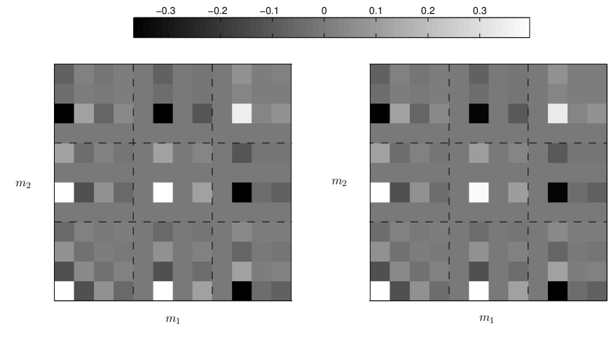
Figure 2: $2D$ cross-correlations using $3$-band Meyer wavelets. Theoretical results (left); experimental results (right).

We aim here at comparing the obtained theoretical expressions of the two-dimensional cross-covariances with Monte Carlo evaluations of these second-order statistics. We consider a two-dimensional 3-band Meyer dual-tree wavelet decomposition of a white standard Gaussian field of size $756\times 756$. The Monte Carlo study is carried out over $10000$ realizations. The decomposition is performed over $J=2$ resolution levels and the results are provided at the coarsest resolution. The covariance fields are depicted in Fig. 2 as well as the ones derived from (31), (54)-(57). For more readibility, a dashed separation line between the subbands has been added (for a $3$-band decomposition, $9$ covariance fields $(\Gamma_{n_{j,{\mathbf{m}}},n_{j,{\mathbf{m}}}^{\mathrm{H}}}[{\boldsymbol{\ell}}])_{{\boldsymbol{\ell}}\in{\mathbb{Z}}^{2}}$ have to be computed when ${\mathbf{m}}\in\{0,1,2\}^{2}$). We compute these fields for ${\boldsymbol{\ell}}\in\{0,1,2,3\}^{2}$, thus resulting in $16$ covariance values for each subband. Succinctly, each small gray-scaled square represents the intensity of the cross-covariance in a given subband $\mathbf{m}$ at spatial position ${\boldsymbol{\ell}}$. Comparing theoretical results with numerical ones (left and right sides of Fig. 2, respectively), it can be noticed that they are quite similar. In addition, we observe that, due to the separability of the covariance fields and (13), for all ${\mathbf{m}}=(m_{1},m_{2})$ and ${\boldsymbol{\ell}}=(\ell_{1},\ell_{2})$, $(\Gamma_{n_{j,{\mathbf{m}}},n_{j,{\mathbf{m}}}^{\mathrm{H}}}[{\boldsymbol{\ell}}])_{{\boldsymbol{\ell}}\in{\mathbb{Z}}^{2}}$ vanishes when either ($m_{1}\neq 0$ and $\ell_{1}=0$) or ($m_{2}\neq 0$ and $\ell_{2}=0$).

VII Conclusion

In this paper, we have investigated the covariance properties of the $M$-band dual-tree wavelet coefficients of wide-sense stationary 1D and 2D random processes. We have stated a number of results helping to better understand the structure of the correlations introduced by this frame decomposition. These results may be useful in the design of efficient denoising rules using dual-tree wavelet decompositions, when the noise is additive and stationary. In particular, if a pointwise estimator is applied to the pair of primal/dual coefficients at the same location and in the same subband, we have seen that the related components of the noise are uncorrelated. On the contrary, if a block-based estimator is used to take advantage of some spatial neighborhood of the primal and dual coefficients around some given position in a subband, noise correlations generally must be taken into account. Recently, this fact has been exploited in the design of an efficient image denoising method using Stein’s principle, yielding state-of-the-art performance for multichannel image denoising [53, 38]. In future work, it would be interesting to extend our analysis to other classes of random processes. In particular, a similar study could be undertaken for self-similar processes [54, 55] and processes with stationary increments [56, 21].

Finally, we would like to note that the expressions of the cross-correlations between the primal and dual wavelets which have been derived in this paper may be of interest for other problems. Indeed, let

$$T=\begin{bmatrix}D\\ D^{\mathrm{H}}\end{bmatrix}$$

denote the dual-tree wavelet decomposition where $D$ (resp. $D^{\mathrm{H}}$) is the primal (resp. dual) wavelet decomposition. The studied cross-correlations then characterize the “off-diagonal” terms of the operator

$$TT^{*}=\begin{bmatrix}I&D(D^{\mathrm{H}})^{*}\\ D^{\mathrm{H}}D^{*}&I\end{bmatrix},$$

where $A^{*}$ denotes the adjoint of a bounded linear operator $A$. The operator $TT^{*}$ is encountered in the solution of some inverse problems.

Appendix A Proof of Proposition 1

The $M$-band wavelet coefficients of the noise are given by

$$\forall m\in{\mathbb{N}}_{M}, \forall k\in{\mathbb{Z}},\qquad$$

$$n_{j,m}[k]=\int_{-\infty}^{\infty}n(x)\;\frac{1}{M^{j/2}}\psi_{m}(\frac{x}{M^{j}}-k)\,dx$$

$$n_{j,m}^{\mathrm{H}}[k]=\int_{-\infty}^{\infty}n(x)\;\frac{1}{M^{j/2}}\psi_{m}^{\mathrm{H}}(\frac{x}{M^{j}}-k)\,dx.$$

For all $(m,m^{\prime})\in{\mathbb{N}}^{2}_{M}$ and $(k,k^{\prime})\in{\mathbb{Z}}^{2}$, we have then

$$\mathsf{E}\{n_{j,m}[k]n_{j,m^{\prime}}[k^{\prime}]\}=\int_{-\infty}^{\infty}\int_{-\infty}^{\infty}\mathsf{E}\{n(x)n(x^{\prime})\}\\ \times\frac{1}{M^{j/2}}\psi_{m}(\frac{x}{M^{j}}-k)\frac{1}{M^{j/2}}\psi_{m^{\prime}}(\frac{x^{\prime}}{M^{j}}-k^{\prime})dx\,dx^{\prime}\,.$$ (83)

After the variable change $\tau=x-x^{\prime}$, using the definition of the autocovariance of the noise in (5), we find that

$$\mathsf{E}\{n_{j,m}[k]n_{j,m^{\prime}}[k^{\prime}]\}=\int_{-\infty}^{\infty}\Gamma_{n}(\tau)\\ \Big{(}\int_{-\infty}^{\infty}\frac{1}{M^{j/2}}\psi_{m}(\frac{x}{M^{j}}-k)\frac{1}{M^{j/2}}\psi_{m^{\prime}}(\frac{x-\tau}{M^{j}}-k^{\prime})dx\Big{)}d\tau$$ (84)

which readily yields

$$\mathsf{E}\{n_{j,m}[k]n_{j,m^{\prime}}[k^{\prime}]\}=\int_{-\infty}^{\infty}\Gamma_{n}(\tau)\gamma_{\psi_{m},\psi_{m^{\prime}}}(\frac{\tau}{M^{j}}+k^{\prime}-k)\,d\tau.$$

Note that, in the above derivations, permutations of the integral symbols/expectation have been performed. For these operations to be valid, some technical conditions are required. For example, Fubini’s theorem [57, p. 164] can be invoked provided that

$$\int_{-\infty}^{\infty}\Gamma_{|n|}(\tau)\gamma_{|\psi_{m}|,|\psi_{m^{\prime}}|}(\frac{\tau}{M^{j}}+k^{\prime}-k)\,d\tau<\infty,$$

where $\Gamma_{|n|}$ is the autocovariance of $|n|$.
Relations (7) and (8) follow from similar arguments.

Appendix B Proof of Proposition 2

For all $(m,m^{\prime})\in{\mathbb{N}}_{M}^{2}$, $\forall\tau\in{\mathbb{R}},\qquad$

$$\frac{1}{2\pi}\int_{-\infty}^{\infty}\widehat{\psi}_{m}^{\mathrm{H}}(\omega)\big{(}\widehat{\psi}_{m^{\prime}}^{\mathrm{H}}(\omega))^{*}e^{\imath\omega\tau}\,d\omega=\gamma_{\psi_{m}^{\mathrm{H}},\psi_{m^{\prime}}^{\mathrm{H}}}(\tau).$$

Since the Fourier transform defines an isometry on ${\mathrm{L}}^{2}({\mathbb{R}})$, it can be deduced from (B) that $\gamma_{\psi_{m}^{\mathrm{H}},\psi_{m^{\prime}}^{\mathrm{H}}}$ is in ${\mathrm{L}}^{2}({\mathbb{R}})$ and its Fourier transform is $\omega\mapsto\widehat{\psi}_{m}^{\mathrm{H}}(\omega)\big{(}\widehat{\psi}_{m^{\prime}}^{\mathrm{H}}(\omega))^{*}$. According to (3) and (4), when $m=m^{\prime}=0$ or $mm^{\prime}\neq 0$, the latter function is equal to $\omega\mapsto\widehat{\psi}_{m}(\omega)\big{(}\widehat{\psi}_{m^{\prime}}(\omega))^{*}$, thus showing that $\gamma_{\psi_{m}^{\mathrm{H}},\psi_{m^{\prime}}^{\mathrm{H}}}=\gamma_{\psi_{m},\psi_{m^{\prime}}}$. The equality of the covariance sequences defined by (6) and (7) straightforwardly follows.

When $mm^{\prime}\neq 0$, the Fourier transform of $\gamma_{\psi_{m},\psi_{m^{\prime}}^{\mathrm{H}}}$ is equal to $\omega\mapsto\imath\,\mathrm{sign}(\omega)\widehat{\psi}_{m}(\omega)\widehat{\psi}_{m^{\prime}}^{*}(\omega)$ whose conjuguate is the Fourier transform of $-\gamma_{\psi_{m^{\prime}},\psi_{m}^{\mathrm{H}}}$. This proves (11), which combined with (8) leads to

$$\forall\ell\in{\mathbb{Z}},\\ \Gamma_{n_{j,m},n_{j,m^{\prime}}^{\mathrm{H}}}[\ell]=-\int_{-\infty}^{\infty}\Gamma_{n}(x)\gamma_{\psi_{m}^{\prime},\psi_{m}^{\mathrm{H}}}\left(-\frac{x}{M^{j}}+\ell\right)dx.$$ (85)

After a variable change and using the fact that $\Gamma_{n}$ is an even function, we obtain (12).

Consider now the Fourier transform $\omega\mapsto\widehat{\psi}_{0}(\omega)(\widehat{\psi}_{0}^{\mathrm{H}}(\omega))^{*}$ of $\gamma_{\psi_{0},\psi_{0}^{\mathrm{H}}}$. For all $\omega\geq 0$, there exists $k\in{\mathbb{N}}$ such as $\omega\in[2k\pi,2(k+1)\pi)$ and, from (4), we get

$$\widehat{\psi}_{0}(\omega)(\widehat{\psi}_{0}^{\mathrm{H}}(\omega))^{*} =(-1)^{k}e^{\imath(d+\frac{1}{2})\omega}\;|\widehat{\psi}_{0}(\omega)|^{2}$$

$$=e^{\imath(2d+1)\omega}\widehat{\psi}_{0}(-\omega)(\widehat{\psi}_{0}^{\mathrm{H}}(-\omega))^{*}.$$

For symmetry reasons, the equality between the first and last terms extends to all $\omega\in{\mathbb{R}}$. Coming back to the time domain, we find

$$\forall\tau\in{\mathbb{R}},\qquad\gamma_{\psi_{0},\psi_{0}^{\mathrm{H}}}(\tau)=\gamma_{\psi_{0},\psi_{0}^{\mathrm{H}}}(-\tau-2d-1).$$

This shows the symmetry of $\gamma_{\psi_{0},\psi_{0}^{\mathrm{H}}}$ w.r.t. $-d-1/2$. Eq. (8) then yields

$$\forall\ell\in{\mathbb{Z}},$$

$$\Gamma_{n_{j,0},n_{j,0}^{\mathrm{H}}}[\ell] =\int_{-\infty}^{\infty}\Gamma_{n}(x)\gamma_{\psi_{0},\psi_{0}^{\mathrm{H}}}\left(-\frac{x}{M^{j}}+\ell-2d-1\right)dx$$

$$=\int_{-\infty}^{\infty}\Gamma_{n}(x)\gamma_{\psi_{0},\psi_{0}^{\mathrm{H}}}\left(\frac{x}{M^{j}}+\ell-2d-1\right)dx$$

$$=\Gamma_{n_{j,0},n_{j,0}^{\mathrm{H}}}[-\ell+2d+1].$$

Appendix C White noise case

Recall that a white noise is not a process with finite variance, but a generalized random process [58, 59]. As such, some caution must be taken in the application of (6)-(8). More precisely, if $n$ is a white noise, its autocovariance can be viewed as the limit as $\epsilon>0$ tends to 0 of

$$\Gamma_{n^{\epsilon}}(\tau)=\frac{\sigma^{2}}{\sqrt{2\pi}\epsilon}\exp(-\frac{\tau^{2}}{2\epsilon^{2}}),\qquad\tau\in{\mathbb{R}}.$$

Formula (8) can then be used, yielding for all $(m,m^{\prime})\in{\mathbb{N}}_{M}^{2}$ and $(j,\ell)\in{\mathbb{Z}}^{2}$,

$$\Gamma_{n_{j,m}^{\epsilon},n_{j,m^{\prime}}^{\epsilon{\mathrm{H}}}}[\ell]=\\ \sigma^{2}\int_{-\infty}^{\infty}\frac{1}{\sqrt{2\pi}}\exp(-\frac{x^{2}}{2})\,\gamma_{\psi_{m},\psi_{m^{\prime}}^{\mathrm{H}}}\left(\frac{\epsilon x}{M^{j}}-\ell\right)dx.$$ (86)

Since $\psi_{m}$ and $\psi_{m^{\prime}}^{\mathrm{H}}$ are in ${\mathrm{L}}^{2}({\mathbb{R}})$, $\gamma_{\psi_{m},\psi_{m^{\prime}}^{\mathrm{H}}}$ is a bounded continuous function. By applying Lebesgue dominated convergence theorem, we deduce that

$$\Gamma_{n_{j,m},n_{j,m^{\prime}}^{\mathrm{H}}}[\ell]=\lim_{\epsilon\to 0}\Gamma_{n_{j,m}^{\epsilon},n_{j,m^{\prime}}^{\epsilon{\mathrm{H}}}}[\ell]$$

$$=\sigma^{2}\int_{-\infty}^{\infty}\frac{1}{\sqrt{2\pi}}\exp(-\frac{x^{2}}{2})\,\lim_{\epsilon\to 0}\gamma_{\psi_{m},\psi_{m^{\prime}}^{\mathrm{H}}}\left(\frac{\epsilon x}{M^{j}}-\ell\right)dx$$

$$=\sigma^{2}\gamma_{\psi_{m},\psi_{m^{\prime}}^{\mathrm{H}}}(-\ell)\int_{-\infty}^{\infty}\frac{1}{\sqrt{2\pi}}\exp(-\frac{x^{2}}{2})dx$$

which leads to (15). Equations (14) are similarly obtained by further noticing that, due to the orthonormality property, $\gamma_{\psi_{m},\psi_{m^{\prime}}}(-\ell)=\gamma_{\psi_{m}^{\mathrm{H}},\psi_{m^{\prime}}^{\mathrm{H}}}(-\ell)=\delta_{m-m^{\prime}}\delta_{\ell}$.

Appendix D Proof of Proposition 3

From (25) and (26) defining the unitary transform applied to the detail noise coefficients $(n_{j,{\mathbf{m}}}[{\mathbf{k}}])_{{\mathbf{k}}\in{\mathbb{Z}}^{2}}$ and $(n_{j,{\mathbf{m}}}^{\mathrm{H}}[{\mathbf{k}}])_{{\mathbf{k}}\in{\mathbb{Z}}^{2}}$:

$$\mathsf{E}\{w_{j,{\mathbf{m}}}[{\mathbf{k}}] w_{j,{\mathbf{m}}}[{\mathbf{k}}^{\prime}]\}=$$

$$\frac{1}{2}\Big{(}\mathsf{E}\{n_{j,{\mathbf{m}}}[{\mathbf{k}}]n_{j,{\mathbf{m}}}[{\mathbf{k}}^{\prime}]\}+\mathsf{E}\{n_{j,{\mathbf{m}}}[{\mathbf{k}}]n_{j,{\mathbf{m}}}^{\mathrm{H}}[{\mathbf{k}}^{\prime}]\}$$

$$+\mathsf{E}\{n_{j,{\mathbf{m}}}^{\mathrm{H}}[{\mathbf{k}}]n_{j,{\mathbf{m}}}[{\mathbf{k}}^{\prime}]\}+\mathsf{E}\{n_{j,{\mathbf{m}}}^{\mathrm{H}}[{\mathbf{k}}]n_{j,{\mathbf{m}}}^{\mathrm{H}}[{\mathbf{k}}^{\prime}]\}\Big{)}.$$

Using (24) and the evenness of $\Gamma_{n_{j,{\mathbf{m}}},n^{\mathrm{H}}_{j,{\mathbf{m}}}}$, one can easily deduce (27). Concerning (28), we proceed in the same way, taking into account the relation:

$$\mathsf{E}\{w_{j,{\mathbf{m}}}^{\mathrm{H}}[{\mathbf{k}}] w_{j,{\mathbf{m}}}^{\mathrm{H}}[{\mathbf{k}}^{\prime}]\}=$$

$$\frac{1}{2}\Big{(}\mathsf{E}\{n_{j,{\mathbf{m}}}[{\mathbf{k}}]n_{j,{\mathbf{m}}}[{\mathbf{k}}^{\prime}]\}-\mathsf{E}\{n_{j,{\mathbf{m}}}[{\mathbf{k}}]n_{j,{\mathbf{m}}}^{\mathrm{H}}[{\mathbf{k}}^{\prime}]\}$$

$$-\mathsf{E}\{n_{j,{\mathbf{m}}}^{\mathrm{H}}[{\mathbf{k}}]n_{j,{\mathbf{m}}}[{\mathbf{k}}^{\prime}]\}+\mathsf{E}\{n_{j,{\mathbf{m}}}^{\mathrm{H}}[{\mathbf{k}}]n_{j,{\mathbf{m}}}^{\mathrm{H}}[{\mathbf{k}}^{\prime}]\}\Big{)}.$$

Finally, noting that

$$\mathsf{E}\{w_{j,{\mathbf{m}}}[{\mathbf{k}}] w_{j,{\mathbf{m}}}^{\mathrm{H}}[{\mathbf{k}}^{\prime}]\}=$$

$$\frac{1}{2}\Big{(}\mathsf{E}\{n_{j,{\mathbf{m}}}[{\mathbf{k}}]n_{j,{\mathbf{m}}}[{\mathbf{k}}^{\prime}]\}-\mathsf{E}\{n_{j,{\mathbf{m}}}[{\mathbf{k}}]n_{j,{\mathbf{m}}}^{\mathrm{H}}[{\mathbf{k}}^{\prime}]\}$$

$$+\mathsf{E}\{n_{j,{\mathbf{m}}}^{\mathrm{H}}[{\mathbf{k}}]n_{j,{\mathbf{m}}}[{\mathbf{k}}^{\prime}]\}-\mathsf{E}\{n_{j,{\mathbf{m}}}^{\mathrm{H}}[{\mathbf{k}}]n_{j,{\mathbf{m}}}^{\mathrm{H}}[{\mathbf{k}}^{\prime}]\}\Big{)}$$

and, invoking the same arguments, we see that $w_{j,{\mathbf{m}}}[{\mathbf{k}}]$ and $w_{j,{\mathbf{m}}}^{\mathrm{H}}[{\mathbf{k}}^{\prime}]$ are uncorrelated random variables.

Appendix E Proof of Proposition 4

Since $\psi_{m}\in{\mathrm{L}}^{2}({\mathbb{R}})$, we have

$$\forall\tau\in{\mathbb{R}},\\ \gamma_{\psi_{m},\psi_{m}}(\tau)=\frac{1}{2\pi}\int_{-\infty}^{\infty}|\widehat{\psi}_{m}(\omega)|^{2}e^{\imath\omega\tau}\,d\omega.$$ (87)

Furthermore, $|\widehat{\psi}_{m}|^{2}$ is $2N_{m}+1$ times continuously differentiable and for all $q\in\{0,\ldots,2N_{m}+1\}$, $(|\widehat{\psi}_{m}|^{2})^{(q)}\in{\mathrm{L}}^{1}({\mathbb{R}})$. It can be deduced [60][p. 158–159] that

$$\forall\tau\in{\mathbb{R}},\\ (-\imath\tau)^{2N_{m}+1}\gamma_{\psi_{m},\psi_{m}}(\tau)=\frac{1}{2\pi}\int_{-\infty}^{\infty}(|\widehat{\psi}_{m}|^{2})^{(2N_{m}+1)}(\omega)\,e^{\imath\omega\tau}\,d\omega$$ (88)

which leads to

$$\forall\tau\in{\mathbb{R}},\\ |\tau|^{2N_{m}+1}|\gamma_{\psi_{m},\psi_{m}}(\tau)|\leq\frac{1}{2\pi}\int_{-\infty}^{\infty}\big{|}(|\widehat{\psi}_{m}|^{2})^{(2N_{m}+1)}(\omega)\big{|}\,d\omega.$$ (89)

Let us now consider the cross-correlation functions $\gamma_{\psi_{m},\psi_{m}^{\mathrm{H}}}$ with $m\neq 0$. Similarly, when $m\neq 0$, we have

$$\forall\tau\in{\mathbb{R}},\\ \gamma_{\psi_{m},\psi_{m}^{\mathrm{H}}}(\tau)=\frac{1}{2\pi}\int_{-\infty}^{\infty}\alpha(\omega)|\widehat{\psi}_{m}(\omega)|^{2}e^{\imath\omega\tau}\,d\omega,$$ (90)

where $\alpha(\omega)=\imath\,\mathrm{sign}(\omega)$. The function $\omega\mapsto\alpha(\omega)|\widehat{\psi}_{m}(\omega)|^{2}$ is $2N_{m}+1$ times continuously differentiable on ${\mathbb{R}}^{*}$, where its derivative of order $q\in\{0,\ldots,2N_{m}+1\}$ is

$$(\alpha|\widehat{\psi}_{m}|^{2})^{(q)}=\alpha\;(|\widehat{\psi}_{m}|^{2})^{(q)}.$$ (91)

Due to the fact that $|\widehat{\psi}_{m}(\omega)|^{2}=O(\omega^{2N_{m}})$ as $\omega\to 0$, we have for all $q\in\{0,\ldots,2N_{m}-1\}$, $(|\widehat{\psi}_{m}|^{2})^{(q)}(0)=0$. From (91), we deduce that the function $(\alpha|\widehat{\psi}_{m}|^{2})^{(q)}$ admits limits on the left side and on the right side of 0, which are both equal to 0. This allows to conclude that $\alpha|\widehat{\psi}_{m}|^{2}$ is $2N_{m}-1$ times continuously differentiable on ${\mathbb{R}}$, its $2N_{m}-1$ first derivatives vanishing at 0. Besides, $(\alpha|\widehat{\psi}_{m}|^{2})^{(2N_{m}-1)}$ is continuously differentiable on $(-\infty,0]$ and on $[0,\infty)$ ($(\alpha|\widehat{\psi}_{m}|^{2})^{(2N_{m})}$ may be discontinuous at 0). Using the same arguments as for $\gamma_{\psi_{m},\psi_{m}}$, this allows us to claim that

$$\forall\tau\in{\mathbb{R}},$$

$$(-\imath\tau)^{2N_{m}}\gamma_{\psi_{m},\psi_{m}^{\mathrm{H}}}(\tau)=\frac{1}{2\pi}\int_{-\infty}^{\infty}\alpha(\omega)(|\widehat{\psi}_{m}|^{2})^{(2N_{m})}(\omega)e^{\imath\omega\tau}\,d\omega$$

$$=-\frac{1}{\pi}\int_{0}^{\infty}(|\widehat{\psi}_{m}|^{2})^{(2N_{m})}(\omega)\sin(\omega\tau)\,d\omega.$$ (92)

We can note that $\lim_{\omega\to\infty}(|\widehat{\psi}_{m}|^{2})^{(2N_{m})}(\omega)\in{\mathbb{R}}$ as it is equal to $(|\widehat{\psi}_{m}|^{2})^{(2N_{m})}_{+}(0)+\int_{0}^{\infty}(|\widehat{\psi}_{m}|^{2})^{(2N_{m}+1)}(\nu)\,d\nu$ where $(|\widehat{\psi}_{m}|^{2})^{(2N_{m})}_{+}(0)$ denotes the right-hand side derivative of order $2N_{m}$ of $|\widehat{\psi}_{m}|^{2}$ at 0. Since $(|\widehat{\psi}_{m}|^{2})^{(2N_{m})}\in{\mathrm{L}}^{1}([0,\infty))$, the previous limit is necessarily zero. Using this fact and integrating by part in (92), we find that, for all $\tau\in{\mathbb{R}}$,

$$\tau\int_{0}^{\infty}(|\widehat{\psi}_{m}|^{2})^{(2N_{m})}(\omega)\sin(\omega\tau)\,d\omega=(|\widehat{\psi}_{m}|^{2})^{(2N_{m})}_{+}(0)\\ +\int_{0}^{\infty}(|\widehat{\psi}_{m}|^{2})^{(2N_{m}+1)}(\omega)\cos(\omega\tau)\,d\omega.$$ (93)

Combining this expression with (92), we deduce that

$$\forall\tau\in{\mathbb{R}},\\ |\tau|^{2N_{m}+1}|\gamma_{\psi_{m},\psi_{m}^{\mathrm{H}}}(\tau)|\leq\frac{1}{\pi}\Big{(}\int_{0}^{\infty}|(|\widehat{\psi}_{m}|^{2})^{(2N_{m}+1)}(\omega)|\,d\omega\\ +|(|\widehat{\psi}_{m}|^{2})^{(2N_{m})}_{+}(0)|\Big{)}.$$ (94)

Let us now study the case when $m=0$. Eq. (90) still holds, but as shown by (4), $\alpha$ takes a more complicated form:

$$\forall k\in{\mathbb{Z}},\;\forall\omega\in[2k\pi,2(k+1)\pi),\\ \alpha(\omega)=\begin{cases}(-1)^{k}e^{\imath(d+\frac{1}{2})\omega}&\mbox{if $k\geq 0$}\\ (-1)^{k+1}e^{\imath(d+\frac{1}{2})\omega}&\mbox{otherwise.}\end{cases}$$ (95)

So, the function $\alpha$ as well as its derivatives of any order now exhibit discontinuities at $2k\pi$ where $k\in{\mathbb{Z}}^{*}$. However, from (1) and the low-pass condition $\widehat{\psi}_{0}(0)=1$, we have, for all $m\neq 0$,

$$H_{m}(\omega)=O(\omega^{N_{m}}),\qquad\mbox{as $\omega\to 0$.}$$

As a consequence of the para-unitary condition (2), we get

$$\sum_{m=0}^{M-1}|H_{m}(\omega)|^{2}=M$$

and

$$\sum_{p=0}^{M-1}|H_{0}(\omega+p\frac{2\pi}{M})|^{2}=M$$

which allows to deduce that

$$\forall p\in{\mathbb{N}}^{\star}_{M},\qquad H_{0}(\omega+p\frac{2\pi}{M})=O(\omega^{N_{0}}).$$

From (1), it can be concluded that

$$\forall k\in{\mathbb{Z}}^{*},\;\widehat{\psi}_{0}(\omega+2k\pi)=O(\omega^{N_{0}}),\;\mbox{as $\omega\to 0$.}$$ (96)

The derivatives of order $q\in\{0,\ldots,2N_{0}+1\}$ of $\alpha|\widehat{\psi}_{0}|^{2}$ over ${\mathbb{R}}\setminus\{2k\pi,k\in{\mathbb{Z}}^{*}\}$ are given by

$$(\alpha|\widehat{\psi}_{0}|^{2})^{(q)}=\sum_{\ell=0}^{q}\binom{q}{\ell}(\alpha)^{(\ell)}(|\widehat{\psi}_{0}|^{2})^{(q-\ell)},$$

where

$$\forall k\in{\mathbb{Z}},\;\forall\omega\in(2k\pi,2(k+1)\pi),\\ \alpha^{(\ell)}(\omega)=\begin{cases}(-1)^{k}\imath^{\ell}(d+\frac{1}{2})^{\ell}\;e^{\imath(d+\frac{1}{2})\omega}&\mbox{if $k\geq 0$}\\ (-1)^{k+1}\imath^{\ell}(d+\frac{1}{2})^{\ell}\;e^{\imath(d+\frac{1}{2})\omega}&\mbox{otherwise.}\end{cases}$$ (97)

We deduce that, for all $q\in\{0,\ldots,2N_{0}+1\}$, $(\alpha|\widehat{\psi}_{0}|^{2})^{(q)}\in{\mathrm{L}}^{1}({\mathbb{R}})$. Furthermore, combining (96) with (E) allows us to show that, for all $q\in\{0,\ldots,2N_{0}-1\}$, the derivative of order $q$ of $\alpha|\widehat{\psi}_{0}|^{2}$ at $2k\pi$, $k\in{\mathbb{Z}}^{*}$, is defined and equal to 0. Consequently, $\alpha|\widehat{\psi}_{0}|^{2}$ is $2N_{0}-1$ times continuously differentiable on ${\mathbb{R}}$ while $(\alpha|\widehat{\psi}_{0}|^{2})^{(2N_{0}-1)}$ is continuously differentiable on $\cup_{k\in{\mathbb{Z}}}(2k\pi,2(k+1)\pi)$. Similarly to the case $m\neq 0$, this leads to

$$\forall\tau\in{\mathbb{R}},$$

$$(-\imath\tau)^{2N_{0}}\gamma_{\psi_{0},\psi_{0}^{\mathrm{H}}}(\tau)=\frac{1}{2\pi}\int_{-\infty}^{\infty}(\alpha|\widehat{\psi}_{0}|^{2})^{(2N_{0})}(\omega)\,e^{\imath\omega\tau}\,d\omega$$

$$=\frac{1}{2\pi}\sum_{k=-\infty}^{\infty}\int_{2k\pi}^{2(k+1)\pi}(\alpha|\widehat{\psi}_{0}|^{2})^{(2N_{0})}(\omega)\,e^{\imath\omega\tau}\,d\omega.$$ (98)

By integration by part, we deduce that

$$\forall\tau\in{\mathbb{R}},$$

$$(-\imath\tau)^{2N_{0}+1}\gamma_{\psi_{0},\psi_{0}^{\mathrm{H}}}(\tau)=\frac{1}{2\pi}$$

$$\qquad\times\Big{(}\int_{-\infty}^{\infty}(\alpha|\widehat{\psi}_{0}|^{2})^{(2N_{0}+1)}(\omega)\,e^{\imath\omega\tau}\,d\omega+\beta\Big{)}$$ (99)

$$\beta=\sum_{k\in{\mathbb{Z}}^{*}}\big{(}(\alpha|\widehat{\psi}_{0}|^{2})^{(2N_{0})}_{+}(2k\pi)-(\alpha|\widehat{\psi}_{0}|^{2})^{(2N_{0})}_{-}(2k\pi)\big{)}\,e^{\imath 2\pi k\tau},$$ (100)

where $(\alpha|\widehat{\psi}_{0}|^{2})^{(2N_{0})}_{+}(\omega_{0})$ (resp. $(\alpha|\widehat{\psi}_{0}|^{2})^{(2N_{0})}_{-}(\omega_{0})$) denotes the right-side (resp. left-side) derivative of order $2N_{0}$ of $\alpha|\widehat{\psi}_{0}|^{2}$ at $\omega_{0}\in{\mathbb{R}}$. We conclude that

$$\forall\tau\in{\mathbb{R}},\quad|\tau|^{2N_{0}+1}|\gamma_{\psi_{0},\psi_{0}^{\mathrm{H}}}(\tau)|=\\ \frac{1}{2\pi}\Big{(}\int_{-\infty}^{\infty}\big{|}(\alpha|\widehat{\psi}_{0}|^{2})^{(2N_{0}+1)}(\omega)\big{|}\,d\omega+|\beta|\Big{)}.$$ (101)

In summary, we have proved that (32) and (33) hold, the constant $C$ being chosen equal to the maximum value of the left-hand side terms in the inequalities (89), (94) and (101).

Appendix F Proof of Proposition 5

Let $m\in{\mathbb{N}}_{M}$. Since $\psi_{m}$ is a unit norm function of ${\mathrm{L}}^{2}({\mathbb{R}})$, the function $\gamma_{\psi_{m},\psi_{m}^{\mathrm{H}}}$ is upper bounded by 1. As $\gamma_{\psi_{m},\psi_{m}^{\mathrm{H}}}$ further satisfies (33), it can be deduced that

$$\forall\tau\in{\mathbb{R}},\qquad|\gamma_{\psi_{m},\psi_{m}^{\mathrm{H}}}(\tau)|\leq\frac{1+C}{1+|\tau|^{2N_{m}+1}}.$$ (102)

The same upper bound holds for $\gamma_{\psi_{m},\psi_{m}}$.

For a white noise, the property then appears as a straightforward consequence of the latter inequality and Eqs. (14) and (15).

Let us next turn our attention to processes with exponentially decaying covariance sequences. From (8), (5) and (102), we deduce that

$$\forall\ell\in{\mathbb{Z}},\qquad\\ |\Gamma_{n_{j,m},n_{j,m}^{\mathrm{H}}}[\ell]|\leq A(1+C)\int_{-\infty}^{\infty}\frac{e^{-\alpha|x|}}{1+|M^{-j}x-\ell|^{2N_{m}+1}}\,dx.$$ (103)

As the left-hand side of (103) corresponds to an even function of $\ell$, without loss of generality, it can be assumed that $\ell\geq 0$. We can decompose the above integral as

$$\int_{-\infty}^{\infty}\frac{e^{-\alpha|x|}}{1+|M^{-j}x-\ell|^{2N_{m}+1}}\,dx\\ =\int_{0}^{\infty}\frac{e^{-\alpha x}}{1+(M^{-j}x+\ell)^{2N_{m}+1}}\,dx\\ +\int_{0}^{\infty}\frac{e^{-\alpha x}}{1+|M^{-j}x-\ell|^{2N_{m}+1}}\,dx\,.$$ (104)

The first integral in the right-hand side can be upper bounded as follows

$$\int_{0}^{\infty}\frac{e^{-\alpha x}}{1+(M^{-j}x+\ell)^{2N_{m}+1}}\,dx\\ \leq(1+\ell^{2N_{m}+1})^{-1}\int_{0}^{\infty}e^{-\alpha x}\,dx\\ =\alpha^{-1}(1+\ell^{2N_{m}+1})^{-1}.$$ (105)

Let $\epsilon\in(0,1)$ be given. The second integral can be decomposed as

$$\int_{0}^{\infty}\frac{e^{-\alpha x}}{1+|M^{-j}x-\ell|^{2N_{m}+1}}\,dx\\ =\int_{0}^{\epsilon M^{j}\ell}\frac{e^{-\alpha x}}{1+(\ell-M^{-j}x)^{2N_{m}+1}}\,dx\\ +\int_{\epsilon M^{j}\ell}^{\infty}\frac{e^{-\alpha x}}{1+|M^{-j}x-\ell|^{2N_{m}+1}}\,dx.$$ (106)

Furthermore, we have

$$\int_{0}^{\epsilon M^{j}\ell} \frac{e^{-\alpha x}}{1+(\ell-M^{-j}x)^{2N_{m}+1}}\,dx$$

$$\leq(1+(1-\epsilon)^{2N_{m}+1}\ell^{2N_{m}+1})^{-1}\int_{0}^{\epsilon M^{j}\ell}e^{-\alpha x}\,dx$$

$$\leq\alpha^{-1}(1-\epsilon)^{-2N_{m}-1}(1+\ell^{2N_{m}+1})^{-1}$$ (107)

$$\int_{\epsilon M^{j}\ell}^{\infty} \frac{e^{-\alpha x}}{1+|M^{-j}x-\ell|^{2N_{m}+1}}\,dx$$

$$\leq\int_{\epsilon M^{j}\ell}^{\infty}e^{-\alpha x}\,dx=\alpha^{-1}e^{-\alpha\epsilon M^{j}\ell}.$$

From the above inequalities, we obtain

$$\forall\ell\in{\mathbb{N}}^{*},\\ |\Gamma_{n_{j,m},n_{j,m}^{\mathrm{H}}}[\ell]|\leq A(1+C)\alpha^{-1}\big{(}(1+(1-\epsilon)^{-2N_{m}-1})\\ \times(1+\ell^{2N_{m}+1})^{-1}+e^{-\alpha\epsilon M^{j}\ell}\big{)}.$$ (108)

As $\lim_{\ell\to\infty}(1+\ell^{2N_{m}+1})e^{-\alpha\epsilon M^{j}\ell}=0$, it readily follows that there exists $\widetilde{C}\in{\mathbb{R}}_{+}$ such that (35) holds.

The left-hand side of (103) being also an upper bound for $|\Gamma_{n_{j,m},n_{j,m}}[\ell]|$, $\ell\neq 0$, (34) is proved at the same time.

Appendix G Proof of Proposition 7

Let us prove (42), the proof of (41) being quite similar. We first note that $\widehat{\psi}_{m}(\widehat{\psi}_{m^{\prime}}^{\mathrm{H}})^{*}$ and therefore $\gamma_{\psi_{m},\psi_{m^{\prime}}^{\mathrm{H}}}$ belong to ${\mathrm{L}}^{2}({\mathbb{R}})$ (see footnote 3). Applying Parseval’s equality to (8), we obtain for all $\ell\in{\mathbb{Z}}$,

$$\Gamma_{n_{j,m},n_{j,m^{\prime}}^{\mathrm{H}}}[\ell]$$

$$=\frac{1}{2\pi}\int_{-\infty}^{\infty}\widehat{\Gamma}_{n}(\omega)\,M^{j}\widehat{\psi}_{m}^{*}(M^{j}\omega)\widehat{\psi}_{m^{\prime}}^{\mathrm{H}}(M^{j}\omega)e^{\imath M^{j}\ell\omega}d\omega$$

$$=\frac{1}{2\pi}\int_{-\infty}^{\infty}\widehat{\Gamma}_{n}\Big{(}\frac{\omega}{M^{j}}\Big{)}\,\widehat{\psi}_{m}^{*}(\omega)\widehat{\psi}_{m^{\prime}}^{\mathrm{H}}(\omega)e^{\imath\ell\omega}d\omega.$$

As $\Gamma_{n}\in{\mathrm{L}}^{1}({\mathbb{R}})$, the spectrum density $\widehat{\Gamma}_{n}$ is a bounded continuous function. According to Lebesgue dominated convergence theorem,

$$\lim_{j\to\infty}\Gamma_{n_{j,m},n_{j,m^{\prime}}^{\mathrm{H}}}[\ell]$$

$$=\frac{1}{2\pi}\int_{-\infty}^{\infty}\lim_{j\to\infty}\widehat{\Gamma}_{n}\Big{(}\frac{\omega}{M^{j}}\Big{)}\,\widehat{\psi}_{m}^{*}(\omega)\widehat{\psi}_{m^{\prime}}^{\mathrm{H}}(\omega)e^{\imath\ell\omega}d\omega$$

$$=\frac{\widehat{\Gamma}_{n}(0)}{2\pi}\int_{-\infty}^{\infty}\widehat{\psi}_{m}^{*}(\omega)\widehat{\psi}_{m^{\prime}}^{\mathrm{H}}(\omega)e^{\imath\ell\omega}d\omega=\widehat{\Gamma}_{n}(0)\gamma_{\psi_{m},\psi_{m^{\prime}}^{\mathrm{H}}}(-\ell).$$

Appendix H Cross-correlations for Meyer wavelets

Substituting (46) in (20), we obtain, for all $\tau\in{\mathbb{R}}$,

$$\gamma_{\psi_{0},\psi_{0}^{\mathrm{H}}}(\tau)= \frac{1}{\pi}\Big{(}\int_{0}^{\pi(1-\epsilon)}\cos{\Big{(}\omega(d+\frac{1}{2}+\tau)\Big{)}}d\omega$$

$$+\int_{\pi(1-\epsilon)}^{\pi(1+\epsilon)} W^{2}\big{(}\frac{\omega}{2\pi\epsilon}-\frac{1-\epsilon}{2\epsilon}\big{)}\cos{\Big{(}\omega(d+\frac{1}{2}+\tau)\Big{)}}d\omega\Big{)}$$

$$= (1-\epsilon)\mathrm{sinc}\Big{(}\pi(1-\epsilon)(d+\frac{1}{2}+\tau)\Big{)}$$

$$+\epsilon\int_{-1}^{1} W^{2}\Big{(}\frac{1+\theta}{2}\Big{)}\cos{\Big{(}\pi(\epsilon\theta+1)\big{(}d+\frac{1}{2}+\tau\big{)}\Big{)}}d\theta.$$ (109)

Using (48), we get

$$\int_{-1}^{0}W^{2}\Big{(}\frac{1+\theta}{2}\Big{)}\cos{\Big{(}\pi(\epsilon\theta+1)\big{(}d+\frac{1}{2}+\tau\big{)}\Big{)}}d\theta\\ =\int_{0}^{1}\cos{\Big{(}\pi(\epsilon\theta-1)\big{(}d+\frac{1}{2}+\tau\big{)}\Big{)}}d\theta\\ -\int_{0}^{1}W^{2}\Big{(}\frac{1+\theta}{2}\Big{)}\cos{\Big{(}\pi(\epsilon\theta-1)\big{(}d+\frac{1}{2}+\tau\big{)}\Big{)}}d\theta.$$ (110)

This allows us to rewrite (109) as

$$\gamma_{\psi_{0},\psi_{0}^{\mathrm{H}}}(\tau)=\mathrm{sinc}\Big{(}\pi(d+\frac{1}{2}+\tau)\Big{)}-\sin{\Big{(}\pi\big{(}d+\frac{1}{2}+\tau\big{)}\Big{)}}\\ \times I_{\epsilon}\Big{(}d+\frac{1}{2}+\tau\Big{)}.$$ (111)

After simplification, (54) follows.

According to (19) and (50), we have for all $m\in\{1,\ldots,M-2\}$ and $\tau\in{\mathbb{R}}^{*}$,

$$\gamma_{\psi_{m},\psi_{m}^{\mathrm{H}}}(\tau)$$

$$= -\frac{1}{\pi}\Big{(}\int_{\pi(m-\epsilon)}^{\pi(m+\epsilon)}W^{2}\Big{(}\frac{m+\epsilon}{2\epsilon}-\frac{\omega}{2\pi\epsilon}\Big{)}\sin(\omega\tau)d\omega$$

$$+\int_{\pi(m+\epsilon)}^{\pi(m+1-\epsilon)}\sin(\omega\tau)d\omega$$

$$+\int_{\pi(m+1-\epsilon)}^{\pi(m+1+\epsilon)}W^{2}\Big{(}\frac{\omega}{2\pi\epsilon}-\frac{m+1-\epsilon}{2\epsilon}\Big{)}\sin(\omega\tau)d\omega\Big{)}$$

$$= \frac{\cos\big{(}\pi(m+1-\epsilon)\tau\big{)}-\cos\big{(}\pi(m+\epsilon)\tau\big{)}}{\pi\tau}$$

$$+\epsilon\int_{-1}^{1}W^{2}\Big{(}\frac{1+\theta}{2}\Big{)}\sin\big{(}\pi(\epsilon\theta-m)\tau\big{)}d\theta$$

$$-\epsilon\int_{-1}^{1}W^{2}\Big{(}\frac{1+\theta}{2}\Big{)}\sin\big{(}\pi(\epsilon\theta+m+1)\tau\big{)}d\theta.$$

By proceeding similarly to (109)-(110), we find

$$\gamma_{\psi_{m},\psi_{m}^{\mathrm{H}}}(\tau)=\big{(}\cos(\pi(m+1)\tau)-\cos(\pi m\tau)\big{)}\Big{(}\frac{1}{\pi\tau}-I_{\epsilon}(\tau)\Big{)}.$$

When $\tau$ is an integer, this expression further simplifies in (56).

Finally, when $m=M-1$, we have, for all $\tau\in{\mathbb{R}}^{*}$,

$$\gamma_{\psi_{M-1},\psi_{M-1}^{\mathrm{H}}}(\tau)$$

$$= -\frac{1}{\pi}\Big{(}\int_{\pi(M-1-\epsilon)}^{\pi(M-1+\epsilon)}W^{2}\Big{(}\frac{M-1+\epsilon}{2\epsilon}-\frac{\omega}{2\pi\epsilon}\Big{)}\sin(\omega\tau)d\omega$$

$$+\int_{\pi(M-1+\epsilon)}^{\pi M(1-\epsilon)}\sin(\omega\tau)d\omega$$

$$+\int_{\pi M(1-\epsilon)}^{\pi M(1+\epsilon)}W^{2}\Big{(}\frac{\omega}{2\pi\epsilon M}-\frac{1-\epsilon}{2\epsilon}\Big{)}\sin(\omega\tau)d\omega\Big{)}$$

$$= \frac{\cos\big{(}\pi M(1-\epsilon)\tau\big{)}-\cos\big{(}\pi(M-1+\epsilon)\tau\big{)}}{\pi\tau}$$

$$+\epsilon\int_{-1}^{1}W^{2}\Big{(}\frac{1+\theta}{2}\Big{)}\sin\big{(}\pi(\epsilon\theta-M+1)\tau\big{)}d\theta$$

$$-\epsilon M\int_{-1}^{1}W^{2}\Big{(}\frac{1+\theta}{2}\Big{)}\sin\big{(}\pi M(\epsilon\theta+1)\tau\big{)}d\theta$$

$$= \frac{\cos\big{(}\pi M\tau\big{)}-\cos\big{(}\pi(M-1)\tau\big{)}}{\pi\tau}+\cos\big{(}\pi(M-1)\tau\big{)}I_{\epsilon}(\tau)$$

$$-\cos(\pi M\tau)I_{M\epsilon}(\tau).$$

This yields (57).

Appendix I Proof of Proposition 8

Let $m\in{\mathbb{N}}^{*}$. Given (19), (60) leads to

$$-\pi\gamma_{\psi_{2m},\psi_{2m}^{\mathrm{H}}}(\tau)= \int_{0}^{\infty}|\widehat{\psi}_{2m}(\omega)|^{2}\;\sin(\omega\tau)\;d\omega$$

$$= \int_{0}^{\infty}|A_{0}(\omega)|^{2}|\widehat{\psi}_{m}(\omega)|^{2}\;\sin(2\omega\tau)\;d\omega$$ (112)

Furthermore, we have

$$|A_{0}(\omega)|^{2} =\sum_{k}\gamma_{a_{0}}[k]\exp(-\imath k\omega)$$

$$=\gamma_{a_{0}}[0]+2\sum_{k=1}^{\infty}\gamma_{a_{0}}[k]\cos(k\omega).$$

Combining this equation with (112) and using classical trigonometric equalities, we obtain

$$\begin{split}-\pi\gamma_{\psi_{2m},\psi_{2m}^{\mathrm{H}}}(\tau)=&\,\gamma_{a_{0}}[0]\int_{0}^{\infty}|\widehat{\psi}_{m}(\omega)|^{2}\sin(2\omega\tau)d\omega\\ +\sum_{k=1}^{\infty}&\gamma_{a_{0}}[k]\Big{(}\int_{0}^{\infty}|\widehat{\psi}_{m}(\omega)|^{2}\sin\big{(}(2\tau-k)\omega\big{)}d\omega\\ &+\int_{0}^{\infty}|\widehat{\psi}_{m}(\omega)|^{2}\sin\big{(}(2\tau+k)\omega\big{)}d\omega\Big{)}\end{split}$$

which, again invoking Relation (19), yields (62). Eq. (63) can be proved similarly starting from (61).

Appendix J Cross-correlations for Haar wavelet

Knowing the expression of the Fourier transform of the Haar scaling function in (67) and using the cross-correlation formula (20), we obtain:

$$\forall\tau\in{\mathbb{R}},\quad\gamma_{\psi_{0},\psi_{0}^{\mathrm{H}}}(\tau)$$

$$=\frac{1}{\pi}\sum_{k=0}^{\infty}(-1)^{k}\int_{2k\pi}^{2(k+1)\pi}\text{sinc}^{2}(\frac{\omega}{2})\;\cos\big{(}\omega\;(\frac{1}{2}+\tau+d)\big{)}\;d\omega$$

$$=\frac{2}{\pi}\sum_{k=0}^{\infty}(-1)^{k}\int_{k\pi}^{(k+1)\pi}\frac{\sin^{2}{(\nu)}}{\nu^{2}}\cos\big{(}\nu\;(1+2\tau+2d)\big{)}\;d\nu.$$ (113)

By integration by part, we find: for all $(\alpha,\beta,\eta)\in{\mathbb{R}}^{3}$,

$$\int_{\alpha}^{\beta}\frac{\sin^{2}(\omega)}{\omega^{2}}\cos(\eta\omega)d\omega$$

$$= \frac{\sin^{2}(\alpha)\cos(\eta\alpha)}{\alpha}-\frac{\sin^{2}(\beta)\cos(\eta\beta)}{\beta}$$

$$+\frac{1}{4}(2+\eta)\int_{\alpha}^{\beta}\frac{\sin\big{(}(2+\eta)\omega\big{)}}{\omega}d\omega-\frac{\eta}{2}\int_{\alpha}^{\beta}\frac{\sin(\eta\omega)}{\omega}d\omega$$

$$+\frac{1}{4}(2-\eta)\int_{\alpha}^{\beta}\frac{\sin\big{(}(2-\eta)\omega\big{)}}{\omega}d\omega$$

$$= \frac{\sin^{2}(\alpha)\cos(\eta\alpha)}{\alpha}-\frac{\sin^{2}(\beta)\cos(\eta\beta)}{\beta}$$

$$+\frac{1}{4}(\eta+2)\int_{\alpha(\eta+2)}^{\beta(\eta+2)}\frac{\sin(\nu)}{\nu}d\nu-\frac{\eta}{2}\int_{\alpha\eta}^{\beta\eta}\frac{\sin(\nu)}{\nu}d\nu$$

$$+\frac{1}{4}(\eta-2)\int_{\alpha(\eta-2)}^{\beta(\eta-2)}\frac{\sin(\nu)}{\nu}d\nu.$$

Combining this result with (113) leads to (69).

On the other hand, according to (68) and (19), we have

$$\forall\tau\in{\mathbb{R}},\\ \gamma_{\psi_{1},\psi_{1}^{\mathrm{H}}}(\tau)=-\frac{1}{\pi}\int_{0}^{\infty}\textrm{sinc}^{2}(\frac{\omega}{4})\;\sin^{2}{(\frac{\omega}{4})}\;\sin(\omega\tau)\;d\omega\,.$$ (114)

In [61, p.459], an expression of $\int_{0}^{\infty}\frac{\sin^{2}{(\alpha x)}\sin^{2}{(\beta x)}\sin{(2\eta x)}dx}{x^{2}}$ with $(\alpha,\beta,\eta)\in({\mathbb{R}}_{+}^{*})^{3}$ is given. Using this relation yields (70) when $\tau>0$. The general expression for $\tau\in{\mathbb{R}}$ follows from the oddness of $\gamma_{\psi_{1},\psi_{1}^{\mathrm{H}}}$.

Appendix K Cross-correlation for the Franklin wavelet

We have, for all $\tau\in{\mathbb{R}}$,

$$\gamma_{\chi,\chi^{\mathrm{H}}}(\tau) =-\frac{1}{\pi}\int_{0}^{\infty}|\widehat{\chi}(\omega)|^{2}\sin(\omega\tau)d\omega$$

$$=-\frac{2}{\pi}\int_{0}^{\infty}\frac{\sin^{8}(\omega)}{\omega^{4}}\sin(2\omega\tau)d\omega.$$

After two successive integrations by part, we obtain

$$\gamma_{\chi,\chi^{\mathrm{H}}}(\tau)= -\frac{4}{3\pi}\Big{(}4\int_{0}^{\infty}\frac{\sin^{7}(\omega)\cos(\omega)\sin(2\omega\tau)}{\omega^{3}}d\omega$$

$$+ \tau\int_{0}^{\infty}\frac{\sin^{8}(\omega)\cos(2\omega\tau)}{\omega^{3}}d\omega\Big{)}$$

$$= -\frac{2}{3\pi}\Big{(}28\int_{0}^{\infty}\frac{\sin^{6}(\omega)\cos^{2}(\omega)\sin(2\omega\tau)}{\omega^{2}}d\omega$$

$$- 2(2+\tau^{2})\int_{0}^{\infty}\frac{\sin^{8}(\omega)\sin(2\omega\tau)}{\omega^{2}}d\omega$$

$$+16\tau\int_{0}^{\infty}\frac{\sin^{7}(\omega)\cos(\omega)\cos(2\omega\tau)}{\omega^{2}}d\omega\Big{)}.$$ (115)

Standard trigonometric manipulations allow us to write:

$$\sin^{6}(\omega)\cos^{2}(\omega)\sin(2\omega\tau)= \frac{1}{8}\sin^{4}(\omega)\Big{(}\sin(2\tau\omega)$$

$$-\frac{1}{2}\sin\big{(}2 (\tau+2)\omega\big{)}-\frac{1}{2}\sin\big{(}2(\tau-2)\omega\big{)}\Big{)}$$

$$\sin^{8}(\omega)\sin(2\omega\tau)= \frac{1}{16}\sin^{4}(\omega)\Big{(}\sin\big{(}2(\tau+2)\omega\big{)}$$

$$+\sin \big{(}2(\tau-2)\omega\big{)}-\sin\big{(}2(\tau+1)\omega\big{)}$$

$$- 4\sin\big{(}2(\tau-1)\omega\big{)}+6\sin(2\tau\omega)\Big{)}$$

$$\sin^{7}(\omega)\cos(\omega)\cos(2\omega\tau)= \frac{1}{16}\sin^{4}(\omega)\Big{(}\sin\big{(}2(\tau-2)\omega\big{)}$$

$$-\sin \big{(}2(\tau+2)\omega\big{)}+2\sin\big{(}2(\tau+1)\omega\big{)}$$

$$- 2\sin\big{(}2(\tau-1)\omega\big{)}\Big{)}.$$

Inserting these expressions in (115) yields

$$3\pi\gamma_{\chi,\chi^{\mathrm{H}}}(\tau)=Q_{0}(\tau)J(\tau)-Q_{1}(\tau)J(\tau+1)-Q_{1}(-\tau)J(\tau-1)\\ +Q_{2}(\tau)J(\tau+2)+Q_{2}(-\tau)J(\tau-2),$$ (116)

where (see [61, p. 459])

$$\forall x\in{\mathbb{R}},\quad J(x) =2\int_{0}^{\infty}\frac{\sin^{4}(\omega)}{\omega^{2}}\sin(2\omega x)d\omega$$

$$=-\frac{3}{2}x\ln|x|+(1+x)\ln|1+x|$$

$$-(1-x)\ln|1-x|-\frac{2+x}{4}\ln|2+x|$$

$$+\frac{2-x}{4}\ln|2-x|$$

and

$$Q_{0}(\tau)=\frac{3}{4}\tau^{2}-2,\;Q_{1}(\tau)=\frac{\tau^{2}}{2}+2\tau+1,\;Q_{2}(\tau)=\frac{1}{8}(\tau+4)^{2}.$$

Simple algebra allows us to prove that (116) is equivalent to (78).

On the other hand, $|\widetilde{A}_{1}(\omega)|^{2}$ can be viewed as the frequency response of a non causal stable digital filter whose transfer function is

$$P_{\widetilde{A}_{1}}(z) =\displaystyle\frac{6(2-\frac{z+z^{-1}}{2})}{\big{(}1+2\big{(}\frac{z+z^{-1}}{2}\big{)}^{2})(2+\frac{z+z^{-1}}{2})}$$

$$=\frac{2\sqrt{3}}{9}\Big{(}\frac{4(2+\sqrt{3})}{z+2+\sqrt{3}}-\frac{4(2-\sqrt{3})}{z+2-\sqrt{3}}$$

$$+ \frac{7(2+\sqrt{3})-4(1+\sqrt{3})z}{z^{2}+2+\sqrt{3}}-\frac{7(2-\sqrt{3})-4(1-\sqrt{3})z}{z^{2}+2-\sqrt{3}}\Big{)}.$$

We next expand $P_{\widetilde{A}_{1}}(z)$ in Laurent series on the holomorphy domain containing the unit circle, that is

$$\mathcal{D}_{P_{\widetilde{A}_{1}}}=\Big{\{}z\in\mathbb{C}\;\mid\;\frac{\sqrt{3}-1}{\sqrt{2}}<|z|<\frac{\sqrt{3}+1}{\sqrt{2}}\Big{\}}.$$

We thus deduce from the partial fraction decomposition of $P_{\widetilde{A}_{1}}(z)$ that

$$P_{\widetilde{A}_{1}}(z)=\frac{2\sqrt{3}}{9}\Big{(}4\sum_{k=-\infty}^{\infty}(-1)^{k}(2-\sqrt{3})^{|k|}z^{-k}\\ +7\sum_{k=-\infty}^{\infty}(-1)^{k}(2-\sqrt{3})^{|k|}z^{-2k}\\ +4(1-\sqrt{3})\sum_{k=0}^{\infty}(-1)^{k}(2-\sqrt{3})^{k}\big{(}z^{2k+1}+z^{-2k-1}\big{)}\Big{)}.$$ (117)

By identifiying the latter expression with $\sum_{k=-\infty}^{\infty}\gamma_{\tilde{a}_{1}}[k]z^{-k}$, (79) is obtained.

Figure 1: A pair of primal (top) and dual (bottom) analysis/synthesis $M$-band para-unitary filter banks.

$m$	1	2	3	4	5	6	7	8	9	10	11	12
$\pi\gamma_{\psi_{m},\psi_{m}^{\mathrm{H}}}(\tau)$	$\frac{1}{2^{3}\tau^{3}}$	$\frac{1}{2^{5}\tau^{3}}$	$-\frac{3}{2^{7}\tau^{5}}$	$\frac{1}{2^{7}\tau^{3}}$	$-\frac{3}{2^{9}\tau^{5}}$	$-\frac{3}{2^{11}\tau^{5}}$	$\frac{45}{2^{14}\tau^{7}}$	$\frac{1}{2^{9}\tau^{3}}$	$-\frac{3}{2^{11}\tau^{5}}$	$-\frac{3}{2^{13}\tau^{5}}$	$\frac{45}{2^{16}\tau^{7}}$	$-\frac{3}{2^{15}\tau^{5}}$

TABLE I: Asymptotic form of $\gamma_{\psi_{m},\psi_{m}^{\mathrm{H}}}(\tau)$ as $|\tau|\to\infty$ for Walsh-Hadamard wavelets.

	$\gamma_{\psi_{0},\psi_{0}^{\mathrm{H}}}$				$\gamma_{\psi_{1},\psi_{1}^{\mathrm{H}}}$
Wavelets  $\setminus$  $\ell$	0	1	2	3	1	2	3
Shannon	0.63662	-0.21221	0.12732	$-9.0946\times 10^{-2}$	0.63662	0	0.21221
Meyer $\epsilon=1/3$	0.63216	-0.19916	0.10668	$-6.4166\times 10^{-2}$	0.59378	$-4.1412\times 10^{-2}$	0.11930
Splines order 3	0.62696	-0.18538	8.8582$\times 10^{-2}$	-4.6179$\times 10^{-2}$	0.55078	-5.8322$\times 10^{-2}$	8.2875$\times 10^{-2}$
Splines order 1	0.60142	-0.12891	$3.4815\times 10^{-2}$	$-9.2967\times 10^{-3}$	0.38844	$-5.7528\times 10^{-2}$	$1.8659\times 10^{-2}$
Haar	0.51288	$-1.1338\times 10^{-2}$	$-1.0855\times 10^{-3}$	$-2.6379\times 10^{-4}$	0.10816	$5.6994\times 10^{-3}$	$1.5610\times 10^{-3}$

TABLE II: Theoretical cross-correlation values in the dyadic case ($d=0$).

	$\gamma_{\psi_{0},\psi_{0}^{\mathrm{H}}}$				$\gamma_{\psi_{1},\psi_{1}^{\mathrm{H}}}$
Wavelets  $\setminus$  $\ell$	0	1	2	3	1	2	3
Meyer $3$-band $\epsilon=1/4$	0.63411	-0.20478	0.11530	-7.4822$\times 10^{-2}$	0.62662	0	0.18391
Meyer $4$-band $\epsilon=1/5$	0.63501	-0.20742	0.11950	-8.0293$\times 10^{-2}$	0.63020	0	0.19367
Meyer $5$-band $\epsilon=1/6$	0.63550	-0.20887	0.12184	-8.3419$\times 10^{-2}$	0.63216	0	0.19917
Meyer $6$-band $\epsilon=1/7$	0.63580	-0.20975	0.12327	-8.5357$\times 10^{-2}$	0.63334	0	0.20255
Meyer $7$-band $\epsilon=1/8$	0.63599	-0.21033	0.12421	-8.6637$\times 10^{-2}$	0.63411	0	0.20478
Meyer $8$-band $\epsilon=1/9$	0.63612	-0.21072	0.12486	-8.7525$\times 10^{-2}$	0.63463	0	0.20632

TABLE III: Theoretical values for the first two cross-correlation sequences in the $M$-band Meyer case ($d=0$).

	$\gamma_{\psi_{M-1},\psi_{M-1}^{\mathrm{H}}}$
Wavelets  $\setminus$  $\ell$	1	2	3
Meyer $3$-band $\epsilon=1/4$	-0.58918	-6.0378$\times 10^{-2}$	-0.11965
Meyer $4$-band $\epsilon=1/5$	0.58555	-7.0840$\times 10^{-2}$	0.11961
Meyer $5$-band $\epsilon=1/6$	-0.58278	-7.7359$\times 10^{-2}$	-0.11940
Meyer $6$-band $\epsilon=1/7$	0.58063	-8.1773$\times 10^{-2}$	0.11914
Meyer $7$-band $\epsilon=1/8$	-0.57893	-8.4944$\times 10^{-2}$	-0.11888
Meyer $8$-band $\epsilon=1/9$	0.57755	-8.7324$\times 10^{-2}$	0.11863

TABLE IV: Theoretical values for the last cross-correlation sequence in the $M$-band Meyer case ($d=0$).

$\ell$	1	2	3
$\gamma_{\psi_{2},\psi_{2}^{\mathrm{H}}}$	$6.0560\times 10^{-2}$	$1.5848\times 10^{-3}$	$4.0782\times 10^{-4}$
$\gamma_{\psi_{3},\psi_{3}^{\mathrm{H}}}$	$-4.9162\times 10^{-2}$	$-3.0109\times 10^{-4}$	$-3.4205\times 10^{-5}$
$\gamma_{\psi_{4},\psi_{4}^{\mathrm{H}}}$	3.2069$\times 10^{-2}$	4.0952$\times 10^{-4}$	1.0319$\times 10^{-4}$
$\gamma_{\psi_{5},\psi_{5}^{\mathrm{H}}}$	-2.8899$\times 10^{-2}$	-8.0753$\times 10^{-5}$	-8.7950$\times 10^{-6}$
$\gamma_{\psi_{6},\psi_{6}^{\mathrm{H}}}$	-2.4899$\times 10^{-2}$	-2.6077$\times 10^{-5}$	-2.4511$\times 10^{-6}$
$\gamma_{\psi_{7},\psi_{7}^{\mathrm{H}}}$	2.4297$\times 10^{-2}$	1.0608$\times 10^{-5}$	4.8118$\times 10^{-7}$

TABLE V: Theoretical cross-correlation values in the Walsh-Hadamard case.

		$\gamma_{\psi_{0},\psi_{0}^{\mathrm{H}}}$				$\gamma_{\psi_{1},\psi_{1}^{\mathrm{H}}}$
Wavelets	$j$ $\setminus$ $\ell$	0	1	2	3	0	1	2	3
	$1$	0.63538	-0.21134	0.12586	-9.1515$\times 10^{-2}$	9.97$\times 10^{-6}$	0.63680	-1.7137$\times 10^{-4}$	0.21165
Shannon	$2$	0.63558	-0.21347	0.12970	-8.7908$\times 10^{-2}$	2.6426$\times 10^{-6}$	0.63404	7.0561$\times 10^{-4}$	0.21210
	$3$	0.63467	-0.20732	0.13168	-9.0116$\times 10^{-2}$	-1.0078$\times 10^{-4}$	0.63846	-1.2410$\times 10^{-3}$	0.20975
	$1$	0.63091	-0.19828	0.10517	-6.4650$\times 10^{-2}$	1.8257$\times 10^{-5}$	0.61092	-1.2433$\times 10^{-2}$	0.15307
Meyer	$2$	0.63112	-0.20043	0.10903	-6.1060$\times 10^{-2}$	-7.5431$\times 10^{-6}$	0.59115	-4.0881$\times 10^{-2}$	0.11888
$\epsilon=1/3$	$3$	0.62971	-0.19391	0.11084	-6.3378$\times 10^{-2}$	4.0868$\times 10^{-4}$	0.59522	-4.2624$\times 10^{-2}$	0.11651
	$1$	0.62587	-0.18459	8.7088$\times 10^{-2}$	-4.6635$\times 10^{-2}$	-1.4511$\times 10^{-4}$	0.58458	-1.2651$\times 10^{-2}$	0.12557
Splines	$2$	0.62606	-0.18679	9.1068$\times 10^{-2}$	-4.3124$\times 10^{-2}$	1.9483$\times 10^{-4}$	0,54841	-5.8083$\times 10^{-2}$	8.2386$\times 10^{-2}$
order $3$	$3$	0.62398	-0.17984	9.2793$\times 10^{-2}$	-4.5682$\times 10^{-2}$	1.2400$\times 10^{-3}$	0.55204	-5.9368$\times 10^{-2}$	8.0105$\times 10^{-2}$
	$1$	0.60016	-0.12749	3.2975$\times 10^{-2}$	-9.7419$\times 10^{-3}$	-4.5287$\times 10^{-4}$	0.47691	1.6224$\times 10^{-2}$	6.9681$\times 10^{-2}$
Splines	$2$	0.60059	-0.13045	3.7613$\times 10^{-2}$	-6.5441$\times 10^{-3}$	6.6358$\times 10^{-4}$	0.38507	-5.7502$\times 10^{-2}$	1.8042$\times 10^{-2}$
order $1$	$3$	0.59771	-0.12303	3.9388$\times 10^{-2}$	-9.3208$\times 10^{-3}$	2.2725 $\times 10^{-3}$	0.38958	-5.8143$\times 10^{-2}$	1.6160$\times 10^{-2}$
	$1$	0.50297	-3.3557$\times 10^{-3}$	-1.1706$\times 10^{-3}$	2.7788$\times 10^{-4}$	3.8368$\times 10^{-4}$	0.22455	7.2451$\times 10^{-2}$	4.6418$\times 10^{-2}$
Haar	$2$	0.50966	-1.0083$\times 10^{-2}$	7,2357$\times 10^{-6}$	1.5087$\times 10^{-3}$	-1.2135$\times 10^{-3}$	9.9745$\times 10^{-2}$	5.1371$\times 10^{-3}$	1.0847$\times 10^{-3}$
	$3$	0.51023	-8.3267$\times 10^{-3}$	2.7936$\times 10^{-3}$	7.0343$\times 10^{-5}$	1.2329$\times 10^{-3}$	0.10703	6.7651$\times 10^{-3}$	2.2422$\times 10^{-3}$
	$1$	0.59822	-0.12059	2.3566$\times 10^{-2}$	-3.3325$\times 10^{-3}$	-5.0189$\times 10^{-4}$	0.46392	2.1155$\times 10^{-2}$	6.1137$\times 10^{-2}$
Symlets 8	$2$	0.59899	-0.12432	2.8865$\times 10^{-2}$	-2.8960$\times 10^{-4}$	6.7795$\times 10^{-4}$	0.36368	-5.7692$\times 10^{-2}$	9.7533$\times 10^{-3}$
	$3$	0.59654	-0.11703	3.0357$\times 10^{-2}$	-2.8071$\times 10^{-3}$	1.8568$\times 10^{-3}$	0.37012	-5.8376$\times 10^{-2}$	6.9416$\times 10^{-3}$

TABLE VI: Cross-correlation estimates in the dyadic case ($d=0$).

		$\gamma_{\psi_{0},\psi_{0}^{\mathrm{H}}}$				$\gamma_{\psi_{1},\psi_{1}^{\mathrm{H}}}$
Wavelets	$j$ $\setminus$ $\ell$	0	1	2	3	0	1	2	3
Meyer	1	0.63337	-0.20549	0.11431	-7.1877$\times 10^{-2}$	-6.8977$\times 10^{-4}$	0.62533	-1.3630$\times 10^{-4}$	0.18236
$3$-band	2	0.63284	-0.19932	0.11938	-7.5331$\times 10^{-2}$	-1.7781$\times 10^{-4}$	0.63013	1.2830$\times 10^{-3}$	0.18409
$\epsilon=1/4$	3	0.63886	-0.19987	0.11763	-6.6380$\times 10^{-2}$	-3.9622$\times 10^{-4}$	0.61503	8.4042$\times 10^{-4}$	0.17519
Meyer	1	0.63383	-0.20856	0.12176	-7.7150$\times 10^{-2}$	2.1961$\times 10^{-5}$	0.62739	7.6636$\times 10^{-4}$	0.19339
$4$-band	2	0.63648	-0.19903	0.11757	-7.7337$\times 10^{-2}$	4.8821$\times 10^{-4}$	0.62676	3.8876$\times 10^{-3}$	0.18683
$\epsilon=1/5$	3	0.64642	-0.19651	0.12202	-6.9984$\times 10^{-2}$	2.3054$\times 10^{-3}$	0.63384	-1.6254$\times 10^{-3}$	0.19233
Meyer	1	0.63338	-0.20818	0.12534	-8.0594$\times 10^{-2}$	8.6373$\times 10^{-4}$	0.62902	8.3871$\times 10^{-4}$	0.1981
$5$-band	2	0.64020	-0.20288	0.12135	-7.3844$\times 10^{-2}$	5.3607$\times 10^{-4}$	0.62230	4.6651$\times 10^{-4}$	0.19093
$\epsilon=1/6$	3	0.6566	-0.19609	0.12891	-7.6061$\times 10^{-2}$	-2.8654$\times 10^{-3}$	0.62281	-4.7324$\times 10^{-3}$	0.19364
Meyer	1	0.63403	-0.20818	0.12711	-8.2124$\times 10^{-2}$	4.5293$\times 10^{-4}$	0.63229	-1.9919$\times 10^{-3}$	0.20228
$6$-band	2	0.64471	-0.20716	0.13141	-8.4914$\times 10^{-2}$	3.7150$\times 10^{-4}$	0.62450	6.5942$\times 10^{-4}$	0.20313
$\epsilon=1/7$	3	0.66409	-0.19532	0.14401	-9.3486$\times 10^{-2}$	2.0490$\times 10^{-3}$	0.63619	1.5614$\times 10^{-2}$	0.17595
Meyer	1	0.63323	-0.20781	0.12663	-8.3335$\times 10^{-2}$	1.5731$\times 10^{-3}$	0.63528	-8.6821$\times 10^{-4}$	0.20509
$7$-band	2	0.64286	-0.20057	0.12881	-8.1995$\times 10^{-2}$	-1.6505$\times 10^{-4}$	0.62782	-7.9119$\times 10^{-3}$	0.20007
$\epsilon=1/8$	3	0.68445	-0.1845	0.12065	-9.0295$\times 10^{-2}$	-5.9955$\times 10^{-3}$	0.62572	-5.3033$\times 10^{-2}$	0.17409
Meyer	1	0.63426	-0.20592	0.12928	-8.6766$\times 10^{-2}$	-2.1756$\times 10^{-4}$	0,63658	-1.3977$\times 10^{-3}$	0.20385
$8$-band	2	0.64743	-0.19970	0.12725	-7.7096$\times 10^{-2}$	1.4856$\times 10^{-3}$	0.63725	-2.4313$\times 10^{-3}$	0.20396
$\epsilon=1/9$	3	0.69342	-0.20505	0.11257	-6.0075$\times 10^{-2}$	-3.6363$\times 10^{-3}$	0.61590	1.3830$\times 10^{-2}$	0.22112
	1	0.59148	-0.11001	1.9635$\times 10^{-2}$	2.4318$\times 10^{-3}$	-6.6559$\times 10^{-6}$	0.36856	-6.0858$\times 10^{-2}$	8.4608$\times 10^{-5}$
AC	2	0.59855	-0.10412	1.6012$\times 10^{-2}$	1.8921$\times 10^{-4}$	-7.1462$\times 10^{-3}$	0.37379	-5.8026$\times 10^{-2}$	-4.4309$\times 10^{-3}$
$4$-band	3	0.60057	-9.5335$\times 10^{-2}$	2.0094$\times 10^{-2}$	7.6430$\times 10^{-3}$	2.5313$\times 10^{-3}$	0.37514	-5.6207$\times 10^{-2}$	6.8164$\times 10^{-3}$
		$\gamma_{\psi_{2},\psi_{2}^{\mathrm{H}}}$				$\gamma_{\psi_{3},\psi_{3}^{\mathrm{H}}}$
	1	-1.9012$\times 10^{-4}$	-0.34054	5.5692$\times 10^{-2}$	4.6899$\times 10^{-5}$	-5.5011$\times 10^{-5}$	0.36755	4.1274$\times 10^{-2}$	5.6594$\times 10^{-2}$
AC	2	1.0139$\times 10^{-3}$	-0.32275	5.4137$\times 10^{-2}$	-6.7903$\times 10^{-3}$	3.6460$\times 10^{-3}$	0.18371	-4.1645$\times 10^{-2}$	6.8637$\times 10^{-3}$
$4$-band	3	6.8587$\times 10^{-3}$	-0.32199	4.5083$\times 10^{-2}$	-9.7023$\times 10^{-3}$	8.3037$\times 10^{-3}$	0.19070	-3.7675$\times 10^{-2}$	-4.5919$\times 10^{-4}$
	1	2.4712$\times 10^{-4}$	0.20479	6.9476$\times 10^{-2}$	4.4200$\times 10^{-2}$	-1.8669$\times 10^{-4}$	-6.1810$\times 10^{-2}$	-1.2677$\times 10^{-3}$	2.4199$\times 10^{-5}$
Hadamard	2	3.5680$\times 10^{-3}$	5.9530$\times 10^{-2}$	-5.3171$\times 10^{-3}$	4.3827$\times 10^{-3}$	6.2437$\times 10^{-4}$	-5.0635$\times 10^{-2}$	4.6773$\times 10^{-3}$	-8.7358$\times 10^{-3}$
	3	1.1391$\times 10^{-2}$	5.9541$\times 10^{-2}$	8.3376$\times 10^{-4}$	-1.4604$\times 10^{-3}$	1.9009$\times 10^{-3}$	-5.5798$\times 10^{-2}$	-5.7086$\times 10^{-3}$	-1.1253$\times 10^{-2}$

TABLE VII: Cross-correlation estimates in the $M$-band case ($d=0$).

		$\gamma_{\psi_{M-1},\psi_{M-1}^{\mathrm{H}}}$
Wavelet	$j$ $\setminus$ $\ell$	0	1	2	3
	1	5.2467$\times 10^{-6}$	0.63606	2.0952$\times 10^{-3}$	0.21261
Shannon	2	5.9145$\times 10^{-6}$	0.63592	-4.1893$\times 10^{-3}$	0.21083
$4$-band	3	-1.2667$\times 10^{-4}$	0.62746	-5.7616$\times 10^{-3}$	0.2020
Meyer	1	4.1334$\times 10^{-4}$	-0.60986	-2.5395$\times 10^{-2}$	-0.16095
$3$-band	2	3.9059$\times 10^{-4}$	-0.58694	-6.1089$\times 10^{-2}$	-0.11754
$\epsilon=1/4$	3	3.5372$\times 10^{-3}$	-0.5879	-5.1057$\times 10^{-2}$	-0.11499
Meyer	1	3.9730$\times 10^{-4}$	0.60845	-2.9936$\times 10^{-2}$	0.16111
$4$-band	2	-1.3788$\times 10^{-3}$	0.58530	-7.5797$\times 10^{-2}$	0.11985
$\epsilon=1/5$	3	1.0644$\times 10^{-3}$	0.57418	-7.6790$\times 10^{-2}$	0.10690
Meyer	1	-7.2077$\times 10^{-6}$	-0.60862	-3.4588$\times 10^{-2}$	-0.16162
$5$-band	2	-3.2301$\times 10^{-3}$	-0.58482	-8.6826$\times 10^{-2}$	-0.11844
$\epsilon=1/6$	3	-8.8877$\times 10^{-3}$	-0.56937	-9.3811$\times 10^{-2}$	-0.11512
Meyer	1	8.2632$\times 10^{-4}$	0.60806	-3.7209$\times 10^{-2}$	0.16215
$6$-band	2	-1.2448$\times 10^{-3}$	0.58023	-8.3257$\times 10^{-2}$	0.11022
$\epsilon=1/7$	3	5.5425$\times 10^{-3}$	0.58196	-8.4671$\times 10^{-2}$	0.12368
Meyer	1	2.7863$\times 10^{-4}$	-0.60863	-3.9804$\times 10^{-2}$	-0.16443
$7$-band	2	-5.9703$\times 10^{-3}$	-0.57749	-9.9056$\times 10^{-2}$	-0.11228
$\epsilon=1/8$	3	1.8490$\times 10^{-3}$	-0.58901	-6.4289$\times 10^{-2}$	-0.13516
Meyer	1	-2.5084$\times 10^{-4}$	0.60811	-4.1611$\times 10^{-2}$	0.16612
$8$-band	2	1.0345$\times 10^{-3}$	0.57216	-9.4172$\times 10^{-2}$	0.12014
$\epsilon=1/9$	3	-1.0777$\times 10^{-2}$	0.56259	-0.12183	0.10776

TABLE VIII: Estimation of the last cross-correlation sequence for $M$-band Shannon and Meyer wavelets.

Wavelets	$\setminus$  $\ell$	-3	-2	-1	0	1	2	3
Meyer 2-band	$\gamma_{\psi_{0},\psi_{1}^{\mathrm{H}}}(\ell)$	9.1502$\times 10^{-2}$	-0.10848	0.11800	-0.11800	0.10848	-9.1502$\times 10^{-2}$	7.0491$\times 10^{-2}$
$\epsilon=1/3$	$\gamma_{\psi_{1},\psi_{0}^{\mathrm{H}}}(\ell)$	-8.1258$\times 10^{-2}$	0.10073	-0.11434	0.11924	-0.11434	0.10073	-8.1258$\times 10^{-2}$
Splines	$\gamma_{\psi_{0},\psi_{1}^{\mathrm{H}}}(\ell)$	-8.2660$\times 10^{-2}$	0.13666	-0.18237	0.18237	-0.13666	8.2660$\times 10^{-2}$	-4.5433$\times 10^{-2}$
order $3$	$\gamma_{\psi_{1},\psi_{0}^{\mathrm{H}}}(\ell)$	6.1604$\times 10^{-2}$	-0.10838	0.16319	-0.18941	0.16319	-0.10838	6.1604$\times 10^{-2}$
Haar	$\gamma_{\psi_{0},\psi_{1}^{\mathrm{H}}}(\ell)$	-9.2323$\times 10^{-3}$	-2.2034$\times 10^{-2}$	-0.16656	0.44127	-0.16656	-2.2034$\times 10^{-2}$	-9.2323$\times 10^{-3}$
	$\gamma_{\psi_{1},\psi_{0}^{\mathrm{H}}}(\ell)$	-3.1567$\times 10^{-3}$	-1.9621$\times 10^{-2}$	0.35401	-0.35401	1.9621$\times 10^{-2}$	3.1567$\times 10^{-3}$	1.0758$\times 10^{-3}$
Meyer	$\gamma_{\psi_{0},\psi_{1}^{\mathrm{H}}}(\ell)$	-8.4807$\times 10^{-2}$	8.8904$\times 10^{-2}$	-8.8904$\times 10^{-2}$	8.4807$\times 10^{-2}$	-7.7120$\times 10^{-2}$	6.6763$\times 10^{-2}$	-5.4904$\times 10^{-2}$
$3$-band	$\gamma_{\psi_{1},\psi_{0}^{\mathrm{H}}}(\ell)$	6.0944$\times 10^{-2}$	-7.2206$\times 10^{-2}$	8.1363$\times 10^{-2}$	-8.7347$\times 10^{-2}$	8.9428$\times 10^{-2}$	-8.7347$\times 10^{-2}$	8.1363$\times 10^{-2}$
$\epsilon=1/4$	$\gamma_{\psi_{1},\psi_{2}^{\mathrm{H}}}(\ell)$	-6.3891$\times 10^{-2}$	-7.4738$\times 10^{-2}$	-8.3192$\times 10^{-2}$	-8.8252$\times 10^{-2}$	-8.9297$\times 10^{-2}$	-8.6196$\times 10^{-2}$	-7.9333$\times 10^{-2}$
Meyer	$\gamma_{\psi_{0},\psi_{1}^{\mathrm{H}}}(\ell)$	6.5090$\times 10^{-2}$	-6.9156$\times 10^{-2}$	7.1274$\times 10^{-2}$	-7.1274$\times 10^{-2}$	6.9156$\times 10^{-2}$	-6.5090$\times 10^{-2}$	5.9394$\times 10^{-2}$
$4$-band	$\gamma_{\psi_{1},\psi_{0}^{\mathrm{H}}}(\ell)$	-6.2421$\times 10^{-2}$	6.7350$\times 10^{-2}$	-7.0473$\times 10^{-2}$	7.1543$\times 10^{-2}$	-7.0473$\times 10^{-2}$	6.7350$\times 10^{-2}$	-6.2421$\times 10^{-2}$
$\epsilon=1/5$	$\gamma_{\psi_{1},\psi_{2}^{\mathrm{H}}}(\ell)$	6.0949$\times 10^{-2}$	6.6274$\times 10^{-2}$	6.9878$\times 10^{-2}$	7.1475$\times 10^{-2}$	7.0939$\times 10^{-2}$	6.8312$\times 10^{-2}$	6.3804$\times 10^{-2}$
	$\gamma_{\psi_{2},\psi_{3}^{\mathrm{H}}}(\ell)$	-6.5090$\times 10^{-2}$	6.9156$\times 10^{-2}$	-7.1274$\times 10^{-2}$	7.1274$\times 10^{-2}$	-6.9156$\times 10^{-2}$	6.5090$\times 10^{-2}$	-5.9394$\times 10^{-2}$

TABLE IX: Inter-band cross-correlation values for some wavelet families. We recall that Property (12) holds and that, for $M$-band Meyer wavelets $\gamma_{\psi_{m},\psi_{m^{\prime}}^{\mathrm{H}}}$ is zero when $|m-m^{\prime}|>1$.

References

• [1] S. Mallat, A wavelet tour of signal processing.   San Diego, CA, USA: Academic Press, 1998.
• [2] S. Cambanis and E. Masry, “Wavelet approximation of deterministic and random signals: convergence properties and rates,” IEEE Trans. on Inform. Theory, vol. 40, no. 4, pp. 1013–1029, Jul. 1994.
• [3] I. Daubechies, “The wavelet transform, time-frequency localization and signal analysis,” IEEE Trans. on Inform. Theory, vol. 36, no. 5, pp. 961–1005, Sep. 1990.
• [4] R. Gribonval and M. Nielsen, “Sparse representations in unions of bases,” IEEE Trans. on Inform. Theory, vol. 49, no. 12, pp. 3320–3325, Dec. 2003.
• [5] P. G. Casazza, “The art of frame theory,” Taiwanese J. of Math., vol. 15, no. 4, pp. 129–201, 2000.
• [6] R. Coifman and D. Donoho, Translation-invariant de-noising, ser. Lecture Notes in Statistics.   New York, NY, USA: Springer Verlag, 1995, vol. 103, pp. 125–150.
• [7] J.-C. Pesquet, H. Krim, and H. Carfatan, “Time-invariant orthogonal wavelet representations,” IEEE Trans. on Signal Proc., vol. 44, no. 8, pp. 1964–1970, Aug. 1996.
• [8] H. Bölcskei, F. Hlawatsch, and H. G. Feichtinger, “Frame-theoretic analysis of oversampled filter banks,” IEEE Trans. on Signal Proc., vol. 46, no. 12, pp. 3256–3268, Dec. 1998.
• [9] E. P. Simoncelli and H. Farid, “Steerable wedge filters for local orientation analysis,” IEEE Trans. on Image Proc., vol. 5, no. 9, pp. 1377–1382, Sep. 1996.
• [10] M. N. Do and M. Vetterli, “The contourlet transform: an efficient directional multiresolution image representation,” IEEE Trans. on Image Proc., vol. 14, no. 12, pp. 2091–2106, Dec. 2005.
• [11] E. Le Pennec and S. Mallat, “Sparse geometric image representations with bandelets,” IEEE Trans. on Image Proc., vol. 14, no. 4, pp. 423–438, Apr. 2005.
• [12] E. Candès, L. Demanet, D. Donoho, and L. Ying, “Fast discrete curvelet transforms,” SIAM J. on Mult. Model. Simul., vol. 5, no. 3, pp. 861–899, Mar. 2006.
• [13] R. A. Gopinath, “The phaselet transform — an integral redundancy nearly shift-invariant wavelet transform,” IEEE Trans. on Signal Proc., vol. 51, no. 7, pp. 1792–1805, Jul. 2003.
• [14] V. Velisavljević, B. Beferull-Lozano, M. Vetterli, and P. L. Dragotti, “Directionlets: anisotropic multidirectional representation with separable filtering,” IEEE Trans. on Image Proc., vol. 15, no. 7, pp. 1916–1933, Jul. 2006.
• [15] R. Figueras i Ventura, P. Vandergheynst, and P. Frossard, “Low rate and flexible image coding with redundant representations,” IEEE Trans. on Image Proc., vol. 15, no. 3, pp. 726–739, Mar. 2006.
• [16] D. Pastor and R. Gay, “Décomposition d’un processus stationnaire du second ordre. Propriétés statistiques d’ordre 2 des coefficients d’ondelettes et localisation fréquentielle des paquets d’ondelettes,” Traitement du signal, vol. 12, no. 5, pp. 393–420, 1995.
• [17] M. Vanucci and F. Corradi, “Some findings on the covariance structure of wavelet coefficients: theory and models in a Bayesian perspective,” Preprint, 1997.
• [18] D. Leporini and J.-C. Pesquet, “High-order wavelet packets and cumulant field analysis,” IEEE Trans. on Inform. Theory, vol. 45, no. 3, pp. 863–876, Apr. 1999.
• [19] R. Averkamp and C. Houdré, “A note on the discrete wavelet transform of second-order processes,” IEEE Trans. on Inform. Theory, vol. 46, no. 4, pp. 1673–1676, Jul. 2000.
• [20] S. Cambanis and C. Houdré, “On the continuous wavelet transform of second-order random processes,” IEEE Trans. on Inform. Theory, vol. 41, no. 3, pp. 628–642, May 1995.
• [21] R. Averkamp and C. Houdré, “Some distributional properties of the continuous wavelet transform of random processes,” IEEE Trans. on Inform. Theory, vol. 44, no. 3, pp. 1111–1124, May 1998.
• [22] J. E. Fowler, “The redundant discrete wavelet transform and additive noise,” Signal Processing Letters, vol. 12, pp. 629–632, 2005.
• [23] P. Abry and P. Flandrin, “Multiresolution transient detection,” in Proc. Int. Symp. on Time-Freq. and Time-Scale Analysis, Philadelphia, USA, Oct. 1994, pp. 225–228.
• [24] S. C. Olhede and A. T. Walden, “Analytic wavelet thresholding,” Biometrika, vol. 91, pp. 955–973, 2004.
• [25] P. Abry, Ondelettes et turbulences.   Paris, France: Diderot éd., arts et sciences, 1997.
• [26] N. G. Kingsbury, “The dual-tree complex wavelet transform: a new technique for shift invariance and directional filters,” in Proc. IEEE Digital Signal Processing Workshop, no. 86, Bryce Canyon, UT, USA, Aug. 9-12 1998.
• [27] I. W. Selesnick, “Hilbert transform pairs of wavelet bases,” Signal Processing Letters, vol. 8, no. 6, pp. 170–173, Jun. 2001.
• [28] I. W. Selesnick, R. G. Baraniuk, and N. G. Kingsbury, “The dual-tree complex wavelet transform,” IEEE Signal Processing Magazine, vol. 22, no. 6, pp. 123–151, Nov. 2005.
• [29] A. Jalobeanu, L. Blanc-Féraud, and J. Zerubia, “Satellite image debbluring using complex wavelet packets,” Int. J. Comp. Vis., vol. 51, no. 3, pp. 205–217, 2003.
• [30] C. Chaux, L. Duval, and J.-C. Pesquet, “Hilbert pairs of $M$-band orthonormal wavelet bases,” in Proc. Eur. Sig. and Image Proc. Conference, Vienna, Austria, September 6-10, 2004, pp. 1187–1190.
• [31] ——, “$2D$ dual-tree $M$-band wavelet decomposition,” in Proc. Int. Conf. on Acoust., Speech and Sig. Proc., vol. 4, Philadelphia, USA, March 18-23, 2005, pp. 537–540.
• [32] ——, “Image analysis using a dual-tree ${M}$-band wavelet transform,” IEEE Trans. on Image Proc., vol. 15, no. 8, pp. 2397–2412, Aug. 2006.
• [33] O. Rioul and P. Duhamel, “Fast algorithms for discrete and continuous wavelet transforms,” IEEE Trans. on Inform. Theory, vol. 38, no. 2, pp. 569–586, Mar. 1992.
• [34] P. Abry and P. Flandrin, “On the initialization of the discrete wavelet transform algorithm,” Signal Processing Letters, vol. 1, no. 2, pp. 32–34, Feb. 1994.
• [35] B. Wang, Y. Wang, I. Selesnick, and A. Vetro, “An investigation of 3D dual-tree wavelet transform for video coding,” in Proc. Int. Conf. on Image Processing, vol. 2, Singapore, Oct. 24-27 2004, pp. 1317–1320.
• [36] L. Şendur and I. W. Selesnick, “Bivariate shrinkage functions for wavelet-based denoising exploiting interscale dependency,” IEEE Trans. on Signal Proc., vol. 50, no. 11, pp. 2744–2756, November 2002.
• [37] H. Rabbani, M. Vafadust, and S. Gazor, “Image denoising based on a mixture of laplace distributions with local parameters in complex wavelet domain,” in Proc. Int. Conf. on Image Processing, Atlanta, GA, USA, Oct. 8-11 2006, pp. 2597–2600.
• [38] C. Chaux, L. Duval, A. Benazza-Benyahia, and J.-C. Pesquet, “A nonlinear Stein based estimator for multichannel image denoising,” Preprint, 2007, submitted.
• [39] P. Steffen, P. N. Heller, R. A. Gopinath, and C. S. Burrus, “Theory of regular $M$-band wavelet bases,” IEEE Trans. on Signal Proc., vol. 41, no. 12, pp. 3497–3511, Dec. 1993.
• [40] S. Touati and J.-C. Pesquet, “Some results on the wavelet packet decomposition of nonstationary processes,” EURASIP J. Appl. Sign. Proc., no. 11, pp. 1289–1295, Nov. 2002.
• [41] Y. Meyer, Ondelettes et opérateurs. I, ser. Actualités mathématiques.   Paris, France: Hermann, 1990.
• [42] I. Daubechies, Ten Lectures on Wavelets.   Philadelphia, PA, USA: CBMS-NSF, SIAM Lecture Series, 1992.
• [43] B. Tennant and R. M. Rao, “Solution to the orthogonal $M$-channel bandlimited wavelet construction proposition,” in Proc. Int. Conf. on Acoust., Speech and Sig. Proc., vol. 6, Hong Kong, China, April 6-10, 2003, pp. 389–392.
• [44] R. R. Coifman and M. V. Wickerhauser, “Entropy-based algorithms for best-basis selection,” IEEE Trans. on Inform. Theory, vol. 38, no. 2, pp. 713–718, Mar. 1992.
• [45] M. Drmota and J. Rivat, “The sum of digits function of squares,” J. of the London Math. Soc., vol. 72, no. 2, pp. 273–292, 2005.
• [46] J.-P. Allouche, J. Shallit, and J. Sondow, “Summation of series defined by counting blocks of digits,” J. Number Theory, vol. 123, no. 1, pp. 133–143, Mar. 2007.
• [47] P. Franklin, “A set of continuous orthogonal functions,” Math. Annalen, vol. 100, pp. 522–529, 1928.
• [48] J. O. Strömberg, “A modified Franklin system and higher-order spline systems on ${\bf R}^{\rm n}$ as unconditional bases for Hardy spaces,” in Conference in harmonic analysis in honor of Antoni Zygmund, March 23-28, 1981, ser. Wadworth mathematics series, W. Beckner, A. P. Calerón, R. Fefferman, and P. W. Jones, Eds., vol. II.   Belmont, CA, USA: Wadsworth, Inc., 1983, pp. 475–493.
• [49] G. Battle, “A block spin construction of ondelettes. Part I: Lemarié functions,” Comm. Math. Phys., vol. 110, pp. 601–615, 1987.
• [50] P.-G. Lemarié, “Une nouvelle base d’ondelettes de ${L}^{2}({{\mathbb{R}}}^{n})$,” J. de Math. Pures et Appl., vol. 67, pp. 227–236, 1988.
• [51] M. Unser, “Splines, a perfect fit for signal processing,” Signal Processing Magazine, vol. 16, no. 6, pp. 22–38, Nov. 1999.
• [52] O. Alkin and H. Caglar, “Design of efficient $M$-band coders with linear-phase and perfect-reconstruction properties,” IEEE Trans. on Signal Proc., vol. 43, no. 7, pp. 1579–1590, Jul. 1995.
• [53] C. Chaux, L. Duval, A. Benazza-Benyahia, and J.-C. Pesquet, “A new estimator for image denoising using a 2D dual-tree $M$-band wavelet decomposition,” in Proc. Int. Conf. on Acoust., Speech and Sig. Proc., vol. 3, Toulouse, France, May 21-24, 2006, pp. 249–252.
• [54] P. Abry, P. Gonçalvès, and P. Flandrin, “Wavelets, spectrum analysis and $1/f$ processes,” in Wavelets and Statistics, A. Antoniadis and G. Oppenheim, Eds.   Lecture Notes in Statistics, Springer Verlag, 1995, pp. 15–30.
• [55] G. W. Wornell and A. V. Oppenheim, “Wavelet-based representations for a class of self-similar signals with applications to fractal modulation,” IEEE Trans. on Inform. Theory, vol. 38, no. 2, pp. 785–800, Mar. 1992.
• [56] H. Krim and J.-C. Pesquet, “Multiresolution analysis of a class of nonstationary processes,” IEEE Trans. on Inform. Theory, vol. 41, pp. 1010–1020, Jul. 1995.
• [57] W. Rudin, Real and complex analysis, 3rd ed.   Singapore: McGraw-Hill Science, 1987.
• [58] I. M. Guelfand and G. E. Chilov, Distributions Vols.1 & 2.   Paris, France: Dunod, 1962.
• [59] A. M. Yaglom, Correlation theory of stationary and related functions I. Basic results.   New York, USA: Springer-Verlag, 1987.
• [60] L. Schwartz, Analyse IV : applications à la théorie de la mesure.   Paris, France: Hermann, 1997.
• [61] I. S. Gradshteyn and I. M. Ryzhik, Table of integrals, series, and products.   San Diego, USA: Academic Press, 2000.
Refer to caption
$G^{*}_{0}$ $G^{*}_{1}$ $G^{*}_{M-1}$ $\downarrow\!M$ $\downarrow\!M$ $\downarrow\!M$ $\uparrow\!M$ $\uparrow\!M$ $\uparrow\!M$ $G_{0}$ $G_{1}$ $G_{M-1}$ $H^{*}_{0}$ $H^{*}_{1}$ $H^{*}_{M-1}$ $\downarrow\!M$ $\downarrow\!M$ $\uparrow\!M$ $\uparrow\!M$ $\uparrow\!M$ $H_{0}$ $H_{1}$ $H_{M-1}$ $\downarrow\!M$