Confluent Hasse diagrams

Abstract

We show that a transitively reduced digraph has a confluent upward drawing if and only if its reachability relation has order dimension at most two. In this case, we construct a confluent upward drawing with $O(n^{2})$ features, in an $O(n)\times O(n)$ grid in $O(n^{2})$ time. For the digraphs representing series-parallel partial orders we show how to construct a drawing with $O(n)$ features in an $O(n)\times O(n)$ grid in $O(n)$ time from a series-parallel decomposition of the partial order. Our drawings are optimal in the number of confluent junctions they use.

1 Introduction

One of the most important aspects of a graph drawing is that it should be readable: it should convey the structure of the graph in a clear and concise way. Ease of understanding is difficult to quantify, so various proxies for readability have been proposed; one of the most prominent is the number of edge crossings. That is, we should minimize the number of edge crossings in our drawing (a planar drawing, if possible, is ideal), since crossings make drawings harder to read. Another measure of readability is the total amount of ink required by the drawing [1]. This measure can be formulated in terms of Tufte’s “data-ink ratio”  [22, 35], according to which a large proportion of the ink on any infographic should be devoted to information. Thus given two different ways to present information, we should choose the more succinct and crossing-free presentation.

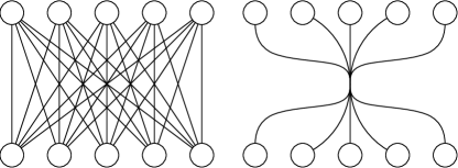
Figure 1: Conventional and confluent drawings of $K_{5,5}$.

Confluent drawing[8, 10, 11, 18, 20, 33, 12] is a style of graph drawing in which multiple edges are combined into shared tracks, and two vertices are considered to be adjacent if a smooth path connects them in these tracks (Figure 1). This style was introduced to reduce crossings, and in many cases it will also improve the ink requirement by representing dense subgraphs concisely. However, it has had a limited impact to date, as there are only a few specialized graph classes for which we can either guarantee the existence of a confluent drawing or test for confluence efficiently. A closely related graph drawing technique, edge bundling [19, 13], differs from confluence in emphasizing the visualization of high level graph structure, but does not necessarily seek to reduce the number of edge crossings.

Hasse diagrams are a type of upward drawing of transitively reduced directed acyclic graphs (DAGs) that have been used since the late 19th century to visualize partially ordered sets. To maximize the readability of Hasse diagrams, as with other types of graph drawing, we would like to draw them without crossings. Thus upward planar graphs (DAGs that can be drawn so that all edges go upwards and no edges cross) have been an important thread of research in graph drawing. A DAG is upward planar if and only if it is a subgraph of a planar st-graph, i.e. a planar DAG with one source and one sink, both on the outer face [7]. Testing upward planarity is NP-complete [15] but for DAGs with a single source or a single sink it may be tested efficiently [21, 4]. However, many DAGs (even planar DAGs such as the one in Figure 2) are not upward planar.

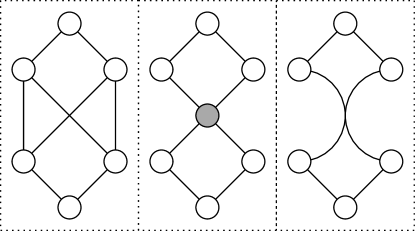
Figure 2: A simple DAG $P$ (left) that is not upward planar, although its underlying graph is planar. Its Dedekind–MacNeille completion (middle) is upward planar, with an added element (shaded). Replacing that element with a junction creates an upward confluent drawing of $P$ (right).

In this paper, we bring these threads together by finding efficient algorithms for upward confluent drawing of transitively reduced DAGs. We show that a graph has an upward confluent drawing if and only if it represents a partial order $P$ with order dimension at most two, and that these drawings correspond to two-dimensional lattices containing $P$. We construct the smallest lattice containing $P$ (its Dedekind–MacNeille completion) in worst-case-optimal time, and draw it confluently in area $O(n^{2})$, using as few confluent junctions as possible. For series-parallel partial orders, the time and number of junctions can be reduced to linear.

Summarizing, we have the following new results:

• We characterize the transitively reduced digraphs with confluent upward drawings: they are the digraphs whose reachability relation has order dimension at most two.

• We construct a confluent upward drawing for any transitively reduced digraph that has one, by constructing the Dedekind–MacNeille completion of the reachability poset and creating confluent junctions corresponding to the added elements in the completion. Our drawings have $O(n^{2})$ junctions and track segments and can be embedded into an $O(n)\times O(n)$ grid in $O(n^{2})$ time. The number of junctions is the minimum possible for any confluent upward drawing of the given digraph.

• For series-parallel partial orders and the corresponding transitively reduced graphs, we show how to construct a confluent drawing with $O(n)$ elements, in an $O(n)\times O(n)$ grid, in $O(n)$ time given a series-parallel decomposition of the partial order.

2 Preliminaries

2.1 Posets and Lattices

Here we review some basic definitions and notation concerning posets and lattices. For more, see e.g. [5, 34]. A partially ordered set (partial order, or poset) $P=(V,\leq)$ is a set $V$ with a reflexive, antisymmetric, and transitive binary relation $\leq$. We adopt the convention that $n=|V|$ unless otherwise stated. We also use $a<b$ to denote that $a\leq b$ and $a\neq b$. We say that $a$ covers $b$ in $P$ if $b<a$ and $\nexists x\in P\mbox{ such that }b<x<a$. Elements $a,b\in P$ are comparable if $a\leq b$ or $b\leq a$; otherwise, we write $a||b$ to indicate that they are incomparable. A total order or linear order is a partial order in which every pair of elements in $P$ is comparable. If $R$ is a set of linear orders $R_{i}$, we can define a poset $P$ as the intersection of $R$: that is, $a\leq b$ in $P$ if and only if $a\leq b$ in every linear order $R_{i}$. If $P$ can be defined from $R$ in this way, then $R$ is called a realizer of $P$. Every partial order $P$ has a realizer; the dimension $\dim(P)$ is the smallest number of linear orders in a realizer of $P$.

If $X\subseteq P$ is any subset of $P$, then an element $a\in P$ is called a lower bound of $X$ if it is less than or equal to every element of $X$. Similarly, an element $b$ is called an upper bound of $X$ if it is greater than or equal to every element of $X$. If $X$ has a lower bound $a$ that belongs to $X$ itself, then $a$ is the (unique) least element in $X$, and similarly if $X$ has an upper bound $b$ that belongs to $X$ then $b$ is the (unique) greatest element in $X$. If the set $A$ of lower bounds of $X$ has a greatest element $a$, then $a$ is the greatest lower bound or infimum of $X$, and similarly if the set $B$ of upper bounds of $X$ has a lowest element $b$ then $b$ is the least upper bound or supremum of $X$. If $P$ itself has an infimum or a supremum, these elements are typically denoted by $0$ and $1$ respectively. If $P$ contains both an infimum and a supremum, it is said to be bounded.

A poset $L$ is a lattice if for every pair of elements $x$ and $y$ in $L$ the set $\{x,y\}$ has both an infimum and a supremum. In this context, the supremum of $\{x,y\}$ is called the meet of $x$ and $y$ and denoted $x\wedge y$, and similarly the infimum is called the join and denoted $x\vee y$. A lattice $L$ is complete if every subset of $L$ has an infimum and supremum in $L$. Every finite lattice is complete and bounded.

2.2 Hasse Diagrams and Upward Planarity

Every poset $P=(V,\leq)$ can be represented by a directed acyclic graph $G$ which has a vertex for each element in $P$ and an edge $uv$ for each pair $(u,v)$ with $u\leq v$ in $P$. However, when we draw a poset it is more common to draw a different DAG, the transitive reduction $G^{\prime}$ of $G$, in which there is an edge from $u$ to $v$ in $G^{\prime}$ if and only if $v$ covers $u$ in $P$. A Hasse diagram of $P$ is an upward drawing of $G^{\prime}$, meaning that the $y$ coordinate of the head of each edge is greater than the $y$ coordinate of the tail of each edge, and each edge is a $y$-monotone curve, so that the drawing “flows” upward from smaller elements to larger elements. In a Hasse diagram, we do not need to explicitly draw the edges as directed edges: the direction of an edge is represented implicitly by the relative position of its endpoints. There is an upward path from $a$ to $b$ in a Hasse diagram of $P$ if and only if $a\leq b$. A poset is planar if it has a Hasse diagram that is upward planar, i.e. its transitive reduction has an upward drawing in which none of the edges intersect except at a shared vertex.

A finite lattice is planar if and only if its transitive reduction is a planar st-graph, a DAG which contains exactly one source $s$ and one sink $t$ both of which belong to the outer face of an upward planar drawing [32]. More generally, any DAG is upward planar if and only if it is a subgraph of a planar st-graph [7]. In the other direction, every planar finite bounded poset must be a lattice [3, 5, 23]. This implies that a two-dimensional bounded poset that is not a lattice (such as the one on the left of Figure 2) cannot have an upward planar drawing, and that planarity (a crossing-free drawing) and two-dimensionality (realization by a pair of linear orders) are distinct for non-lattice posets.

2.3 Lattice Completion of a Poset

The Dedekind–MacNeille completion of a poset $P$ (also called the normal completion or the completion) is the smallest complete lattice containing $P$ [26]. Its construction is based on Dedekind’s construction of the real numbers as Dedekind cuts of rational numbers. For any subset $X$ of $P$, let $X^{-}$ and $X^{+}$ denote the set of lower bounds and upper bounds of $X$ respectively. A cut of $P$ is a pair $A,B\subseteq P$ such that $A^{+}=B$ and $A=B^{-}$; the completion of $P$ has these cuts as its elements. The completion is partially ordered by set containment: if $(A,B)$ and $(C,D)$ are cuts, then $(A,B)\leq(C,D)$ if and only if $A\subseteq C$ and $B\supseteq D$. The element of the completion corresponding to an element $x$ of $P$ is the cut $(\{x\}^{-},\{x\}^{+})$, and the new elements added to $P$ to make it into a lattice come from cuts $(A,B)$ for which $A\cap B=\emptyset$. The completion automatically has the same dimension as the partial order from which it was constructed [31].

Ganter and Kuznetsov [14] give a stepwise algorithm for constructing the completion of $P$. Given a poset $P$ and its completion $L$ they show how to complete a one-element extension of $P$ in time $O(|L|\cdot|P|\cdot\omega(P))$, where $\omega(P)$ denotes the width of $P$. To compute the completion of a large poset, they begin with a single-element poset (whose completion is trivial) and use this subroutine to add elements one at a time; therefore, the total time is $O(|L|\cdot|P|^{2}\cdot\omega(P))$. Nourine and Raynaud [30] give an algorithm with running time $O((|P|+|B|)\cdot|B|\cdot|L|)$ where $B$ is a basis of $P$ (a set of subsets of $P$ which generate $L$). As part of our drawing algorithm, we improve these results in the case of two-dimensional posets: we show for such sets how to construct the completion in time $O(|P|^{2})$, optimal in the worst case since (as we also show) there exist two-dimensional posets whose completion has a quadratic number of elements.

2.4 Confluent Drawing

Confluent drawing is a technique for drawing non-planar diagrams without crossings [8, 10, 11, 18, 20, 33, 12] by merging together groups of edges and drawing them as tracks that, like train tracks, meet smoothly at junction points but do not cross. A confluent drawing consists of a set of labeled points (vertices and junctions) and curves (track segments) in the Euclidean plane, such that the two endpoints of each track segment are vertices or junctions, such that no two track segments intersect except at a shared endpoint, and such that all track segments that meet at a junction share a common tangent line at that point. The graph represented by a confluent drawing has as its vertices the vertices of the drawing; two vertices $u$ and $v$ are adjacent if and only if there is a smooth curve in the plane from $u$ to $v$ that is a union of track segments and that does not pass through any other vertex. (Some papers on confluence require that this curve also be non-self-intersecting but that requirement is irrelevant for upward drawings since monotone curves cannot self-intersect.) An undirected graph $G$ is confluent if and only if there exists a confluent drawing that represents it.

We define a confluent diagram of a poset to be a drawing of its transitive reduction in a way that is both confluent and upwards. In other words, if $G$ is a directed acyclic graph representing a poset $P$, then we define a confluent diagram of $P$ to be an upward confluent drawing of the transitive reduction of $G$ in which all tracks are oriented upwards (monotonic in the $y$ direction), and therefore all smooth curves passing through the tracks are similarly oriented. For each pair of elements $a,b\in P$, the drawing should have a smooth track from $a$ upwards to $b$ if and only if $a$ is covered by $b$. We also require that for each source there exists an unbounded $y$-monotone curve downwards that does not cross the diagram – that is, that each source can be seen from below – and symmetrically that each sink can be seen from above. In the application to visualization of partial orders, this is a natural restriction as it makes the minimal and maximal elements easy to find in the drawing.

3 Drawing Posets of Dimension Two

Let $G$ be a poset with dimension at most two. We now describe an $O(n^{2})$ algorithm to embed a confluent diagram of $P$ in an $O(n)\times O(n)$ grid. That is, we will generate an upward confluent drawing of the transitive reduction of a DAG representing $P$ such that each vertex in the drawing has integer coordinates.

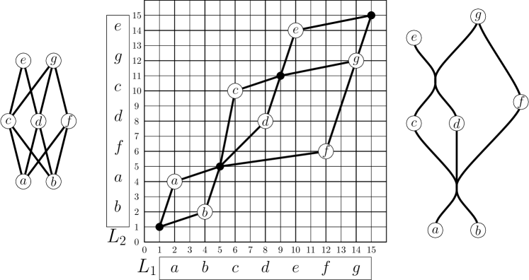
Figure 3: Example of our algorithm. Left: Input poset $P$. Middle: Grid embedding with added points and dominance pairs. Right: Completion points replaced by confluent junctions and rotated $45^{\circ}$.

Our algorithm has three phases. In the first phase, we embed the elements of $P$ in a $(2n+1)\times(2n+1)$ grid. Recall that since $P$ has dimension two, it is realized by two linear orders, which correspond to two different total orderings of the same $n$ elements in $P$. Thus, the first steps of our algorithm are:

1. 1. Find two linear orders $L_{1}$ and $L_{2}$ that realize $P$. This can be done in $O(n^{2})$ time from any graph whose transitive closure is $P$ by Algorithm 1 of Ma and Spinrad [25].

   2. For each element $p$ of $P$, having position $i$ in $L_{1}$ and $j$ in $L_{2}$ with $1\leq i,j\leq n$, place a vertex representing $p$ in the grid with coordinates $(2i,2j)$.

After this step, the even rows and columns in the grid each contain exactly one element of $P$, and the dominance relationship of these points corresponds to the order of the elements in $P$. Recall that for two elements $p$ and $q$ in the plane, $p$ dominates $q$ if and only if $p_{i}\geq q_{i}$ for each coordinate $i$ and $p\neq q$.

In the second phase, we insert additional points representing elements of the completion of $P$; these completion nodes correspond to confluent junctions in the confluent diagram of $P$. We defer to Section 4 the proof that the dominance order on the points generated in the first two phases gives the completion of $P$.

1. For each pair of odd indices $(i,j)\in[3,2n-1]^{2},$ insert a junction in the grid with coordinates $(i,j)$ if all of the following four conditions hold:

   • The poset point with $x$-coordinate $i-1$ has $y$-coordinate less than $j-1$.

   • The point with $x$-coordinate $i+1$ has $y$-coordinate greater than $j+1$.

   • The point with $y$-coordinate $j-1$ has $x$-coordinate less than $i-1$.

   • The point with $y$-coordinate $j+1$ has $x$-coordinate greater than $i+1$.

   In addition if $P$ does not already have a least or a greatest element, then insert invisible points at $(1,1)$ and $(2n+1,2n+1)$ respectively.

In the third phase, we generate the segments of the confluent diagram. These segments correspond to direct dominance pairs of points from the first two phases. It is possible to find all dominance pairs in a set of $N$ points in time $O(N\log N+k)$ [16] where $k$ is the number of dominance pairs, but in our case $N$ may be too large, so this would only lead to an $O(n^{2}\log n)$ time bound. Instead, we leverage the fact that the vertices are embedded in an $O(n)\times O(n)$ grid, and use the following $O(n^{2}+k)$ time method to generate dominance pairs using a stack-based algorithm related to Graham scan within each row. We prove later that the diagram is planar and therefore that the number $k$ of dominance pairs is $O(n^{2})$.

1. For each column $c$ we maintain a value $t_{c}$, the topmost element seen so far in column $c$. Initialize each $t_{c}$ to None.

   Then, for each row $r$ from $1$ to $2n+1$:

   1. Initialize an empty stack $S$.

   2. For each column $c$ from $1$ to $2n+1$:

      1. If there is a vertex or junction $p$ at $(r,c)$, add an edge from every element of $S$ to $p$, add an edge from $t_{c}$ to $p$ (if $t_{c}$ is is not None), and set $t_{c}$ to $p$.

      2. If $t_{c}$ is is not None, pop all items from $S$ whose row number is less than or equal to the row number of $t_{c}$, and push $t_{c}$ onto $S$.

Thus we have computed the coordinates of all elements, confluent junctions, and edges in the confluent diagram. When we render the drawing, we rotate it $45^{\circ}$ counterclockwise to make it upward confluent (Figure 3).

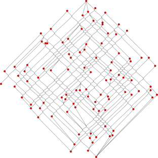
Figure 4: A 100-element partially ordered set, the intersection of two random permutations, drawn as a conventional Hasse diagram with crossings (left), and as a confluent Hasse diagram (right).

Examples of non-confluent and confluent drawings of the same 100-element set are shown in Figure 4. Our Python implementation renders the confluent track segments as cubic Bézier curves with control points at a small fixed distance directly above and below each confluent junction. Two such curves cannot cross each other: for pairs of edges that do not share an endpoint, this follows from the fact that the convex hulls of the control points are disjoint and that the curves lie within the convex hulls, while for pairs of curves that share an endpoint it follows from the fact that the two curves are images of each other under an affine transformation of the plane and that (for pairs of edges sharing an endpoint) the direction that any point on the curve is translated by this affine transformation is transverse to the tangent direction of the curve at that point.

If the input is provided as a realizer rather than as a graph, and its completion has few elements, then it is possible to construct the diagram more efficiently. To do so, construct for each odd-indexed row or column of the integer grid an axis-parallel line segment that passes through a grid point if and only if that point meets two of the four conditions for adding a junction in phase two of our algorithm. The junctions can be recovered as the intersections of these line segments, and we may compute the edges of the diagram using an output-sensitive algorithm for dominance pairs. By using integer searching data structures the total time for this algorithm may be reduced to $O((n+k)\log\log n)$, where $k$ is the number of confluent junctions; we omit the details.

4 Algorithm Correctness and Minimality

In this section we prove that the algorithm of Section 3 is correct and has optimal running time. Our analysis also shows that a poset $P$ has a confluent diagram if and only if it has dimension at most two.

Lemma 4.1 (Baker, Fishburn and Roberts [3]).

Let $P$ be a bounded finite planar poset. Then $P$ is a lattice and has dimension at most 2.

Lemma 4.2.

Let $P$ be a finite poset with a confluent Hasse diagram $D$. Then $\dim(P)\leq 2$, and there exists a two-dimensional lattice $C$ containing $P$ such that the elements of $C\setminus P$ (other than the top and bottom element, if they do not belong to $P$) correspond one-for-one with the confluent junctions of $D$.

Proof.

Replace the confluent junctions of $D$ with vertices, and re-interpret the confluent segments as edges between these vertices. If there is more than one minimal vertex of $P$, add a vertex below all minimal vertices, connected to the minimal vertices by upward edges, and similarly if there is more than one maximal vertex of $P$, add a vertex above all maximal vertices connected to them by edges. The modified drawing is st-planar and hence by Lemma 4.1 represents a lattice, which clearly contains $P$. ∎

Lemma 4.3.

Let $P$ be a finite poset with order dimension at most two, let $C$ be the completion of $P$, and let $S$ be the set of elements of $C\setminus P$ (other than the top and bottom element, if $P$ itself is not bounded). Then the elements of $S$ coincide with the junction points added in phase 2 of our algorithm, and the dominance ordering on these points coincides with the lattice ordering in $C$.

Proof.

In one direction, let $p$ be a junction point added in phase 2 of our algorithm, and $p^{-}$ and $p^{+}$ be the sets of points from phase 1 that are dominated by $p$ and that dominate $p$ respectively. Then it follows from the four conditions according to which phase 2 adds a point that $(p^{-},p^{+})$ forms a cut in $P$. The equivalence of the dominance and lattice orderings on pairs consisting of a junction point and a point from $P$ follows immediately, and the same equivalence for pairs of junction points is also easy to verify.

In the other direction, we must show that we add a junction point for every element of $S$, that is, every cut $(L,U)$ where $L$ has more than one maximal element and $U$ has more than one minimal element. Let $i$ be one less than the minimum $x$-coordinate of a point in $U$, and let $j$ be one less than the minimum $y$-coordinate; then (because the coordinates of points in $P$ are their positions in the two orderings of a realizer) the set $L$ of points dominated by every point in $U$ equals the set of points below and to the left of $(i,j)$. Two of the four conditions of phase 2 are automatically met at $(i,j)$: the points with $x$-coordinate $i+1$ and with $y$-coordinate $j+1$ are both in $U$ and are distinct because $U$ has more than one minimal point. The other two conditions must also be met, for if they were not then the point violating the condition would dominate $L$, contradicting the fact that all points that dominate $L$ belong to $U$. ∎

Theorem 4.4.

A given partial order $P$ has a confluent diagram if and only if $\dim(P)\leq 2$. If $P$ has a confluent diagram, the algorithm of Section 3 computes a valid confluent diagram of $P$, and embeds that diagram in a $O(n)\times O(n)$ grid in worst case optimal $O(n^{2})$ time. The number of confluent junctions in the drawing is the minimum possible for any confluent diagram of $P$.

Proof.

If a poset $P$ has dimension three or more, then so does any lattice containing it, and by Lemma 4.1 and Lemma 4.2 there can be no confluent diagram of $P$. Otherwise, we may assume that $P$ has dimension at most two.

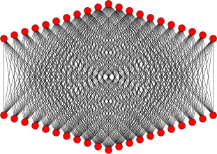
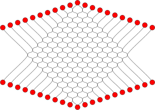
Figure 5: A poset $P$ with $O(n)$ elements and dimension 2 whose completion has size $\Omega(n^{2})$. On the left is the normal Hasse diagram, and on the right is the confluent version as drawn by our algorithm. The two permutations $L_{1}$ and $L_{2}$ generating $P$ are the identity and the permutation $(3n,3n-2,\dots,n;4n+1,n-1,4n,n-2,\dots,3n+2,0;3n+1,3n-1,\dots,n+1)$.

By Lemma 4.3, the dominance ordering on the points computed by our algorithm coincides (except possibly for the removal of the top and bottom elements) with the completion of $P$. In this set of points, there can be no crossing pairs of dominance relations, for if the edges $(L_{1},U_{1})$–$(L_{2},U_{2})$ and $(L_{3},U_{3})$–$(L_{4},U_{4})$ crossed (where $(L_{i},U_{i})$ is a cut either added in the completion or corresponding to an original point of $P$) then $(L_{1}\cup L_{3},U_{2}\cup U_{4})$ would also be a cut whose point would lie between the other four points, contradicting the assumption that these edges represent minimal dominance pairs. Therefore, the diagram constructed by our algorithm is planar, and by Lemma 4.1 it must represent a lattice superset of $P$. The added elements belong to the completion, so the diagram must represent a subset of the completion, and since the completion has no proper lattice subsets it must represent the completion itself. The completion gives the minimum number of added elements (and therefore, by Lemma 4.2, the minimum number of junctions) of any diagram for $P$.

Our algorithm spends $O(n^{2})$ time in its first two phases as it iterates over $O(n^{2})$ grid cells spending constant time per cell. In the third phase, it uses constant time per edge and by planarity there are $O(n^{2})$ edges, so the time is again $O(n^{2})$. This time bound is optimal since (as shown in Figure 5) there exist two-dimensional posets whose completion has $\Omega(n^{2})$ elements. ∎

Although our method produces drawings in a grid of linear dimensions, it may be possible in some cases to compact our drawings into a smaller grid. An algorithm of de la Higuera and Nourine [17] may be used to find the smallest grid into which a drawing produced by our algorithm can be compacted.

Subsequent to our work, a different embedding into lattices has been applied by Czédli [6] to characterize the partial orders of dimension two as being the posets with quasiplanar Hasse diagrams, diagrams in which each incomparable elements has one element on a consistent side of all maximal chains through the other element. The lattices into which Czédli embeds a partial order are semimodular, a property that does not hold for all two-dimensional lattices. Therefore, unlike the Dedekind–MacNeille completion that we use, these lattices do not have a minimal number of elements: a non-semimodular two-dimensional lattice will be drawn with no additional confluent junctions by our algorithm, but will be augmented by additional elements in the method of Czédli.

5 Confluent Drawings of Series-Parallel Posets

Figure 6: A series-parallel poset.

A series-parallel partial order is a poset that can be built up from single elements by two simple composition operations:

• The series composition $P;Q$ of posets $P$ and $Q$ is the order on the set $P\cup Q$ in which $p\leq q$ for every $p\in P$ and $q\in Q$.

• The parallel composition $P||Q$ is the order on $P\cup Q$ in which $p||q$ for every $p\in P$ and $q\in Q$.

Pairs of elements that are both from $P$ or both from $Q$ retain their ordering in the larger set.

Series-parallel partial orders are attractive because many important computational problems can be solved more easily in them than in more general posets, and because they have applications to a wide variety of problems including scheduling [29], concurrency [24], data mining [27], networking [2], and more (see [28]).

Series-parallel partial orders can be represented naturally by a binary tree, known as a decomposition tree of the order. The leaves of the tree correspond to single element sets and the internal nodes of the tree correspond to series or parallel composition operations. As the following theorem shows, given a decomposition tree $T$ for a series-parallel partial order $P$, we can draw the confluent diagram of $P$ in linear time by traversing $T$, performing the corresponding composition operations, and inserting confluent junctions when necessary.

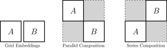
Figure 7: Series and parallel composition operations on two drawings $A$ and $B$.

Theorem 5.1.

Let $P$ be a series-parallel partial order, given as its decomposition tree. Then a confluent diagram of $P$ with a linear number of junctions can be drawn in an $O(n)\times O(n)$ grid in linear time.

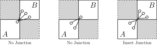
Figure 8: Series composition $A;B$ has a confluent junction if and only if $A$ has no unique upper bound and $B$ has no unique lower bound.

Proof.

We traverse the decomposition tree in post-order, recursively finding embeddings for each subtree. For each tree node, we do the following:

1. If the node is a leaf, then we embed the corresponding element in a single grid cell

2. Otherwise, if the node is a series or parallel node, then we translate the grid embeddings of its two children so that their bounding boxes meet corner to corner (Figure 7).

3. For a series composition $A;B$ we also insert a confluent junction at the shared corner of $A$ and $B$ if and only if $A$ has more than one maximal element and $B$ has more than one minimal element (Figure 8).

By using a linked list of the maximal and minimal nodes for the current subtrees, we can perform these operations in time proportional to the number of leaves in the decomposition tree. Therefore the total time is linear. The size of the grid will be proportional to the size of the decomposition tree, i.e., $O(n)\times O(n)$ ∎

6 Experiments

As a proof of concept for our method, we implemented it and tested how well it performs, in terms of the number of edges or confluent segments drawn and the ink usage of our drawings.

In our experiments, we consider drawing two classes of partial orders separately, first, the special case of series-parallel partial orders and second, all two-dimensional partial orders. We consider several different sizes, and for each size and class we generate graphs of that class and size uniformly at random. We calculate the number of edges and total edge length (ink) in the traditional Hasse diagram and confluent Hasse diagram corresponding to each graph. In the traditional Hasse diagram, each edge is drawn as a straight line between two vertices. In the confluent diagram, an “edge” between two vertices may go through multiple confluent junctions, and multiple “edges” may reuse the same curve incident to a junction. Thus, we count the number of edges in the confluent diagram as the number of confluent segments; we define a confluent segment as a curve between endpoints, where each endpoint is either a vertex or a confluent junction. Each segment is drawn as a cubic bezier curve, but for practical reasons we approximate its length as the length of the three line segments through its control points (Figure 9). Note that this measure will never underestimate the ink used by any edge in our confluent diagram. Because of the quadratic growth in the output complexity of some of our drawings, we limited our experiments to graphs of at most 2048 vertices. For each of the smaller graph sizes, 10,000 permutations were generated uniformly at random. For the larger sizes, we only generated 1000, because of the long run-times, and the low variance of the results.

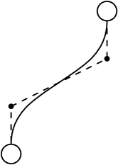
Figure 9: Ink used by each cubic bezier segment is approximated by the straight-line path through its control points.

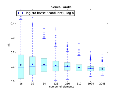
Figure 10: A log-log box plot of the ratio of the number of edges in a traditional Hasse diagram to the number of edges in a confluent Hasse diagram as a function of the number of vertices in upward drawings of series-parallel partial orders. The ratio is normalized by dividing by $\log n$.

Figure 11: A log-log box plot of the ratio of the ink used in a traditional Hasse diagram to the ink used in a confluent Hasse diagram as a function of the number of vertices in upward drawings of series-parallel partial orders. The ratio is normalized by dividing by $\log n$.

In Figure 11 and Figure 11, we compare the average edge count and average ink used for traditional and confluent Hasse diagrams of series-parallel partial orders. The result is that confluent drawings are consistently better than the traditional Hasse diagram in both number of edges and ink used for this class of inputs.

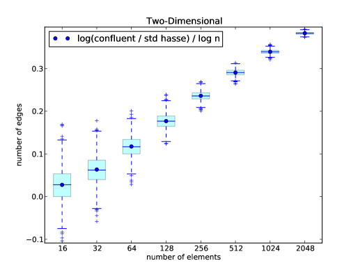
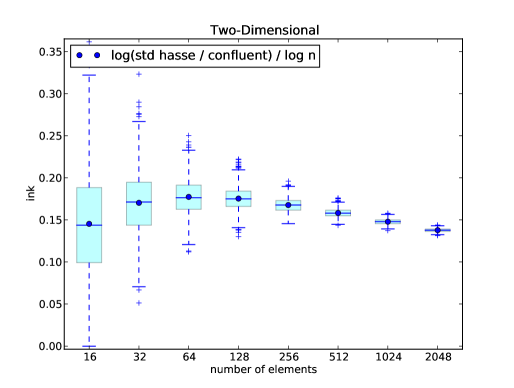
Figure 12: A log-log box plot of the ratio of the number edges in a confluent Hasse diagram to the number of edges in a traditional Hasse diagram as a function of the number of vertices in upward drawings of two-dimensional partial orders. The ratio is normalized by dividing by $\log n$.

Figure 13: A log-log box plot of the ratio of the ink used in a traditional Hasse diagram to the ink used in a confluent Hasse diagram as a function of the number of vertices in upward drawings of two-dimensional partial orders. The ratio is normalized by dividing by $\log n$.

In Figures 13 and 13, we compare the average edge count and average ink used for traditional and confluent Hasse diagrams of two-dimensional partial orders. The result fpr these inputs is that on average the confluent Hasse diagram uses substantially less ink than the traditional Hasse despite the fact that it contains many more edges. Thus, although the confluent Hasse diagram is more complex to render it is also dramatically easier to read.

The reason random two-dimensional partial orders use more edges in a confluent drawing than in a traditional Hasse diagram is that they have a large number of confluent junctions. As we show below, for two-dimensional partial orders generated uniformly at random, the expected number of edges in a Hasse diagram is $\Theta(n\log n)$, but the expected number of confluent junctions in a confluent diagram is $\Theta(n^{2})$. The large number of confluent junctions necessarily implies a drawing with a large number of edges. However, each confluent junction reduces the visual clutter of at least one edge crossing. Thus, while a large number of junctions indicates a drawing with a large number of edges, it also indicates a drawing that is substantially easier to read than the corresponding traditional Hasse diagram.

Graph Generation

Input graphs were sampled uniformly at random from the set of all input graphs for each given size and type (two-dimensional or series-parallel partial orders).

We generate each two-dimensional partial order of size $n$ by generating a permutation on $n$ elements uniformly at random. Each permutation $\pi$ maps the set of elements $L_{n}=[1,n]$ in sorted order to some other order $\pi(L_{n})$. Thus, we have a pair of linear orders $L_{n},\pi(L_{n})$ which define a partial order, since each two-dimensional partial order is realized by pair of linear orders, and by relabeling the elements, any pair of size $n$ linear orders corresponds to $L_{n}$ and some permutation of $L_{n}$.

The set of series-parallel partial orders is a subset of the two-dimensional partial orders. Thus, we generate each series-parallel partial order by sampling uniformly at random from only those permutations that correspond to a series-parallel partial order. Such a permutation can be decomposed uniquely into series and parallel compositions with the constraint that the left argument of each series decomposition is parallel (or an atom) and the left argument of each parallel decomposition is series (or an atom). By means of this decomposition, we may count the number of permutations whose outer composition operation is series (so that the Hasse diagram is connected) by the recurrence relation

$$C_{n}=C_{n-1}+\sum_{i=1}^{n-2}2C_{i}C_{n-i}.$$

The numbers generated by this recurrence are called the little Schroeder numbers. Here $i$ is the size of the left argument of the outer series composition, $n-i$ is the size of its right argument, and the factor of $2$ accounts for the choice of whether to use a series or parallel composition in the right argument. When the right argument has only one element (i.e., when $n-i=1$), this choice is irrelevant, so the term for $i=n-1$ omits the factor of two and is pulled out of the sum as $C_{n-1}$. Our algorithm for generating a random order chooses a random integer in the range from $0$ to $C_{n}-1$, compares it to the partial sums of the terms on the right hand side of the recurrence to determine which value of $i$ to use, and returns the concatenation of two randomly generated permutations of sizes $i$ and $n-i$ (with the first of these two permutations always reversed so that its outer composition operation is parallel rather than series, and the second reversed with probability $1/2$).

Expected edge count.

Eckhardt et al. [9] show that the expected number of edges in a transitively reduced digraph is $\Theta(n\log n)$ in a random graph model where each edge is included in the graph with probability $p$. Our model for generating the graphs is somewhat different, but leads to the same asymptotic bound. There is a clear bijection between any permutation on $n$ elements and a two-dimensional partial order of $n$ elements. Thus, we generate a permutation uniformly at random, which corresponds exactly to a two-dimensional partial order. Under this model each element in the partial order has a pair of coordinates equal to the index and value of the corresponding element in the permutation. There is an edge $(u,v)$ in the Hasse diagram if and only if vertex $v$ covers vertex $u$. That is, $v$ dominates $u$ ($\textit{u.index}<\textit{v.index}$ and $\textit{u.value}<\textit{v.value}$), and there is no third vertex $z$ such that $z$ dominates $u$ and $v$ dominates $z$.

Let $e_{k}$ be the element with index $k$ in column $k$. For each element $e_{j+k}$ in indices $j+k$, $j\in[1,n-k]$, $e_{j}$ covers $e_{k}$ if it is the successor of $e_{k}$ among the $j+1$ elements in indices $[k,k+j]$ ordered by value. Thus, the probability that $e_{j+k}$ covers $e_{k}$ is $1/(j+1)$.

Let $C_{k}$ denote the number of elements which cover element $e_{n-k}$.

$$E[C_{k}]=\sum_{j=1}^{k}\frac{1}{j+1}=\sum_{i=2}^{k+1}\frac{1}{i}=\sum_{i=1}^{k+1}\frac{1}{i}-1=H_{k+1-1}$$

Thus, by linearity of expectation, the expected number of edges in a traditional drawing of a random two-dimensional partial order is

$$\sum_{k=0}^{n-1}E[C_{k}]=\sum_{k=0}^{n-1}H_{k+1}-1=\sum_{k=1}^{n}H_{k}-1=\Theta(n\log n)$$

Expected number of confluent junctions.

Note that each even row and each even column in $[2,2n]$ in the grid contains exactly one point. Let $x_{j}$ denote the $x$-coordinate of the poset point with $y$-coordinate $j$ and let $y_{i}$ denote the $y$ coordinate of the poset point with $x$-coordinate $i$. Let $p^{x}_{j}=(x_{j},j)$ be the unique point with $y$-coordinate $j$, and let $p^{y}_{i}=(i,y_{i})$ be the unique point with $x$-coordinate $i$.

Since we generated the coordinates of the vertices uniformly at random, we can view the $y$ coordinates of the vertices as $n$ uniformly random samples $s_{k}$ without replacement from the integer range $[1,n]$. Thus, the $k$th vertex in the graph is at position $2k,y_{2k}$, given by the value of the $k$th sample $s_{k}=y_{2k}$.

Now consider the probability that a point in a particular row $j$ has a certain $x$ coordinate $x_{j}=i$:

$$Pr(x_{j}=i)=Pr(y_{i}=j)$$

That is, the point in row $j$ has $x$-coordinate $i$ if and only if the unique point in column $i$ (the $\frac{i}{2}th$ sample) has $y$-coordinate $j$. Hence, given that $p_{j}\neq q_{i}$, the values $x_{j}$ and $y_{i}$ are independent.

By construction, for each odd $(i,j)$ in $[3,2n-1]$ there exists a confluent junction at position $(i,j)$ if and only if all of the following conditions hold:

$$y_{i-1} <j-1$$ (1a)

$$y_{i+1} >j+1$$ (1b)

$$x_{j-1} <i-1$$ (1c)

$$x_{j+1} >i+1$$ (1d)

Note that since all the coordinates are integers, we can equivalently state these conditions as follows

$$y_{i-1}<j \quad\text{and}\quad y_{i-1}\neq j-1$$ (2a)

$$y_{i+1}>j \quad\text{and}\quad y_{i+1}\neq j+1$$ (2b)

$$x_{j-1}<i \quad\text{and}\quad x_{j-1}\neq i-1$$ (2c)

$$x_{j+1}>i \quad\text{and}\quad x_{j+1}\neq i+1$$ (2d)

Moreover, the inequality constraint in equation 2a is satisfied if and only if the inequality constraint in equation 2c is satisfied, since there is exactly one vertex in each even row and column. Likewise, the inequality constraints in equations 2b and 2d are equivalent. Hence, we need only keep one of the inequality constraints from each pair of equations, and the inequality constraints can be equivalently stated: $p^{x}_{j-1}\neq p^{y}_{i-1}$ and $p^{x}_{j+1}\neq p^{y}_{i+1}$.

Thus, there exists a junction at $(i,j)$ if and only if

$$x_{j-1}<i<x_{j+1}$$ and

$$y_{i-1}<j<y_{i+1}$$ and

$$p^{x}_{j-1}\neq p^{y}_{i-1}$$ and

$$p^{x}_{j+1}\neq p^{y}_{i+1}$$

That is, the three $x$-coordinates must be in a specific order, the three $y$-coordinates must be in a specific order, and there is a $1/n$ fraction of forbidden coordinates in each of the inequality constraints.

Let $i$ and $j$ be chosen independently and uniformly at random. Then, the probability that $(i,j)$ has a confluent junction is

$$Pr\left(p^{x}_{j-1}\neq p^{y}_{i-1}\right)\cdot Pr\left(p^{x}_{j+1}\neq p^{y}_{i+1}\mid p^{x}_{j-1}\neq p^{y}_{i-1}\right)$$

$$\cdot Pr\left(x_{j-1}<i<x_{j+1}\mid p^{x}_{j-1}\neq p^{y}_{i-1},p^{x}_{j+1}\neq p^{y}_{i+1}\right)$$

$$\cdot Pr\left(y_{i-1}<j<y_{i+1}\mid p^{x}_{j-1}\neq p^{y}_{i-1},p^{x}_{j+1}\neq p^{y}_{i+1},x_{j-1}<i<x_{j+1}\right)$$

$$=(1-\frac{1}{n})^{2}\cdot\frac{1}{6}\cdot\frac{1}{6}$$

Thus, by linearity of expectation, the total expected number of confluent junctions over the whole grid, in a confluent drawing of a random two-dimensional partial order, is $\Theta(n^{2})$.

7 Conclusions

We have designed, analyzed, and implemented an algorithm for drawing confluent Hasse diagrams using a minimum number of confluent junctions. We experimentally verified that confluent diagrams consistently use less ink than the corresponding traditional Hasse diagrams of both two-dimensional and series-parallel partial orders. Confluent diagrams of series-parallel partial orders also use fewer edges. Confluent diagrams of two-dimensional partial orders often use substantially more edges than the corresponding traditional Hasse diagram. However, the larger number of edges used is required by the larger number of confluent junctions required to address all the edge crossings in these graphs. The result is a drawing with more edges but substantially less visual clutter.

Upward planarity may be tested even for non-st-planar graphs that have only one source or one sink; can similar conditions be extended to the case of upward confluent drawings? Can we efficiently find upward planar drawings of graphs that are not transitively reduced? If a partially ordered set must be drawn with crossings, can we use confluence in a principled way to keep the number of crossings small? We leave these questions to future research.

Acknowledgements

This work was supported in part by NSF grants 0830403 and 1217322 and by the Office of Naval Research under grant N00014-08-1-1015.

References

- [1] A. Aeschlimann and J. Schmid. Drawing orders using less ink. Order 9(1):5–13, 1992, doi:10.1007/BF00419035.
- [2] P. Amer, C. Chassot, T. Connolly, M. Diaz, and P. Conrad. Partial-order transport service for multimedia and other applications. IEEE/ACM Transactions on Networking 2(5):440–456, October 1994, doi:10.1109/90.336326.
- [3] K. A. Baker, P. C. Fishburn, and F. S. Roberts. Partial orders of dimension 2. Networks 2(1):11–28, 1972, doi:10.1002/net.3230020103.
- [4] P. Bertolazzi, G. Di Battista, C. Mannino, and R. Tamassia. Optimal upward planarity testing of single-source digraphs. SIAM J. Comput. 27(1):132–169, February 1998, doi:10.1137/S0097539794279626.
- [5] G. Birkhoff. Lattice Theory. AMS Colloquium Publications 25. American Mathematical Society, Providence, 3rd edition, 1967.
- [6] G. Czédli. Quasiplanar diagrams and slim semimodular lattices, arXiv:1212.6904. Unpublished preprint, 2012.
- [7] G. Di Battista and R. Tamassia. Algorithms for plane representations of acyclic digraphs. Theoret. Comput. Sci. 61(2-3):175–198, 1988, doi:10.1016/0304-3975(88)90123-5.
- [8] M. T. Dickerson, D. Eppstein, M. T. Goodrich, and J. Y. Meng. Confluent drawings: visualizing non-planar diagrams in a planar way. J. Graph Algorithms Appl. 9(1):31–52, 2005, doi:10.7155/jgaa.00099.
- [9] S. Eckhardt, A. M. Mühling, and J. Nowak. Fast lowest common ancestor computations in dags. Proc. 15th Eur. Symp. Algorithms (ESA 2007), pp. 705–716. Springer, Lecture Notes in Computer Science 4698, 2007, doi:10.1007/978-3-540-75520-3_62.
- [10] D. Eppstein, M. T. Goodrich, and J. Y. Meng. Delta-confluent drawings. Proc. 13th Int. Symp. Graph Drawing (GD 2005), pp. 165–176. Springer-Verlag, Lecture Notes in Computer Science 3843, 2006, doi:10.1007/11618058_16, arXiv:cs.CG/0510024.
- [11] D. Eppstein, M. T. Goodrich, and J. Y. Meng. Confluent layered drawings. Algorithmica 47(4):439–452, 2007, doi:10.1007/s00453-006-0159-8.
- [12] D. Eppstein, D. Holten, M. Löffler, M. Nöllenburg, B. Speckmann, and K. Verbeek. Strict confluent drawing. Proc. 21st Int. Symp. Graph Drawing (GD 2013), 2013.
- [13] E. Gansner, Y. Hu, S. North, and C. Scheidegger. Multilevel agglomerative edge bundling for visualizing large graphs. Pacific Visualization Symposium (PacificVis), 2011 IEEE, pp. 187–194, March 2011, doi:10.1109/PACIFICVIS.2011.5742389.
- [14] B. Ganter and S. O. Kuznetsov. Stepwise construction of the Dedekind–MacNeille completion. Proc. 6th Int. Conf. Conceptual Structures: Theory, Tools and Applications (ICCS98), pp. 295–302. Springer-Verlag, Lecture Notes in Computer Science 1453, 1998, doi:10.1007/BFb0054922.
- [15] A. Garg and R. Tamassia. On the computational complexity of upward and rectilinear planarity testing. SIAM J. Comput. 31(2):601–625, February 2002, doi:10.1137/S0097539794277123.
- [16] R. H. Güting, O. Nurmi, and T. Ottmann. Fast algorithms for direct enclosures and direct dominances. J. Algorithms 10(2):170–186, 1989, doi:10.1016/0196-6774(89)90011-4.
- [17] C. de la Higuera and L. Nourine. Drawing and encoding two-dimensional posets. Theoret. Comput. Sci. 175(2):293–308, 1997, doi:10.1016/S0304-3975(96)00205-8.
- [18] M. Hirsch, H. Meijer, and D. Rappaport. Biclique edge cover graphs and confluent drawings. Proc. 14th Int. Symp. Graph Drawing (GD 2006), pp. 405–416. Springer-Verlag, Lecture Notes in Computer Science 4372, 2007, doi:10.1007/978-3-540-70904-6_39.
- [19] D. Holten. Hierarchical edge bundles: Visualization of adjacency relations in hierarchical data. IEEE Trans. Visualization and Computer Graphics 12(5):741–748, 2006, doi:10.1109/TVCG.2006.147.
- [20] P. Hui, M. J. Pelsmajer, M. Schaefer, and D. Štefankovič. Train tracks and confluent drawings. Algorithmica 47(4):465–479, 2007, doi:10.1007/s00453-006-0165-x.
- [21] M. D. Hutton and A. Lubiw. Upward planar drawing of single source acyclic digraphs. SIAM J. Comput. 25(2):291–311, 1996, doi:10.1137/S0097539792235906.
- [22] G.-V. Jourdan, I. Rival, and N. Zaguia. Upward drawing on the plane grid using less ink. Proc. 2nd Int. Symp. Graph Drawing (GD 1994), pp. 318–327. Springer-Verlag, Lecture Notes in Computer Science 894, 1995, doi:10.1007/3-540-58950-3_387.
- [23] D. Kelly and I. Rival. Planar lattices. Canad. J. Math. 27(3):636–665, 1975, doi:10.4153/CJM-1975-074-0.
- [24] K. Lodaya and P. Weil. Series-parallel posets: algebra, automata and languages. STACS 98 (Paris, 1998), pp. 555–565. Springer-Verlag, Lecture Notes in Computer Science 1373, 1998, doi:10.1007/BFb0028590.
- [25] T.-H. Ma and J. Spinrad. Transitive closure for restricted classes of partial orders. Order 8(2):175–183, 1991, doi:10.1007/BF00383402.
- [26] H. M. MacNeille. Partially ordered sets. Trans. Amer. Math. Soc. 42(3):416–460, 1937, doi:10.2307/1989739.
- [27] H. Mannila and C. Meek. Global partial orders from sequential data. Proc. 6th ACM SIGKDD Int. Conf. on Knowledge Discovery and Data Mining, pp. 161–168. ACM, KDD ’00, 2000, doi:10.1145/347090.347122.
- [28] R. H. Möhring. Computationally tractable classes of ordered sets. Algorithms and Order, pp. 105–193. Kluwer Academic Publishers, 1989.
- [29] R. H. Möhring and M. W. Schäffter. Scheduling series-parallel orders subject to -communication delays. Parallel Computing 25(1):23–40, 1999, doi:10.1016/S0167-8191(98)00100-8.
- [30] L. Nourine and O. Raynaud. A fast algorithm for building lattices. Inform. Process. Lett. 71(5-6):199–204, 1999, doi:10.1016/S0020-0190(99)00108-8.
- [31] V. Novák. Über eine Eigenschaft der Dedekind-MacNeilleschen Hülle. Math. Ann. 179:337–342, 1969, doi:10.1007/BF01350778.
- [32] C. R. Platt. Planar lattices and planar graphs. J. Combinatorial Theory, Ser. B 21(1):30–39, 1976, doi:10.1016/0095-8956(76)90024-1.
- [33] G. Quercini and M. Ancona. Confluent drawing algorithms using rectangular dualization. Proc. 18th Int. Symp. Graph Drawing (GD 2010), pp. 341–352. Springer-Verlag, Lecture Notes in Computer Science 6502, 2011, doi:10.1007/978-3-642-18469-7_31.
- [34] W. T. Trotter. Combinatorics and partially ordered sets. Johns Hopkins Series in the Mathematical Sciences. Johns Hopkins University Press, Baltimore, MD, 1992, pp. xvi+307. Dimension theory.
- [35] E. R. Tufte. The Visual Display of Quantitative Information. Graphics Press, 1983, p. 197.