KCL-PH-TH/2011-27, LCTS/2011-13, CERN-PH-TH/2011-212

Spin Correlations of $\Lambda{\overline{\Lambda}}$ Pairs

as a Probe of Quark-Antiquark Pair Production

John Ellis¹ and Dae Sung Hwang²

¹Theoretical Particle Physics and Cosmology Group, Physics Department,

King’s College London, Strand, London, UK;

Theory Division, Physics Department, CERN, 1211 Geneva 23, Switzerland

²Department of Physics, Sejong University, Seoul 143–747, South Korea

Abstract

The polarizations of $\Lambda$ and ${\overline{\Lambda}}$ are thought to retain memories of the spins of their parent $s$ quarks and ${\overline{s}}$ antiquarks, and are readily measurable via the angular distributions of their daughter protons and antiprotons. Correlations between the spins of $\Lambda$ and ${\overline{\Lambda}}$ produced at low relative momenta may therefore be used to probe the spin states of $s{\overline{s}}$ pairs produced during hadronization. We consider the possibilities that they are produced in a ³P₀ state, as might result from fluctuations in the magnitude of $\langle{\overline{s}}s\rangle$, a ¹S₀ state, as might result from chiral fluctuations, or a ³S₁ or other spin state, as might result from production by a quark-antiquark or gluon pair. We provide templates for the $p{\overline{p}}$ angular correlations that would be expected in each of these cases, and discuss how they might be used to distinguish $s{\overline{s}}$ production mechanisms in $pp$ and heavy-ion collisions.

PACS numbers: 13.60.Rj Baryon production, 13.87.Fh Fragmentation into hadrons, 13.88.+e Polarization in interactions and scattering, 14.20.Jn Hyperons

1 Introduction

Hadronization proceeds via the production of ${\overline{q}}q$ pairs, that may arise via a combinations of perturbative and non-perturbative mechanisms, such as gluon splitting $g\to{\overline{q}}q$ and fluctuations in the chiral condensate $\langle{\overline{q}}q\rangle$. It is quite possible that the relative importances of these mechanisms may depend on the types of particles colliding, e.g., $pp$ or heavy-ion collisions, and on the kinematic conditions, e.g., low momenta in minimum-bias events or at high $p_{T}$ inside jets.

These mechanisms suggest various different possibilities for the ${\overline{q}}q$ quantum numbers, and in particular their possible spin states. However, it is not immediately apparent how one could determine these spin states by penetrating the ‘hadronization firewall’ via measurements of final-state hadrons. However, one tool for measuring quark spins indirectly is known, namely measuring the polarization states of unstable final-state hyperons, particularly $\Lambda$ baryons [1]. These may be determined by measuring the angular distributions of their decay products, which are in general of the form $(1+P\alpha\cos\theta)$, where $P$ is the polarization and $\alpha\sim 0.6$ in the case of $\Lambda\to p\pi^{-}$ decay [2]. Models of baryon spins based on SU(6) wave functions suggest that the $\Lambda$ ‘remembers’ very well the polarization of its parent $s$ quark, with the accompanying $ud$ pair expected to be in a spin-singlet state [3]. Experimentally, this naive picture seems to be qualitatively correct, e.g., from measurements of $\Lambda$ polarization in final states resulting from $s$ quarks with known spin states [4].

Here we go one step further by proposing to use measurements of the angular correlations between the ${\overline{p}}$ and $p$ produced in the decays of ${\overline{\Lambda}}\Lambda$ pairs to analyze the spin states of parent ${\overline{s}}s$ pairs, specifically those with small relative momenta that could have been produced by a common production reaction.

In the case of perturbative $g\to{\overline{s}}s$ splitting, the final state pair would be in a vector state, that could correspond to a ³S₁ or ³D₁ configuration. The former would dominate if the strange quark mass could be neglected, but the latter is potentially also important for massive quarks, as evidenced by the appearance of a ³D₁ ${\overline{c}}c$ vector meson in $e^{+}e^{-}$ annihilation. Both these configurations are spin-triplet states, so in both cases one might expect the ${\overline{\Lambda}}\Lambda$ pair also to have a spin-triplet configuration. However, whereas in the ³S₁ case the ${\overline{\Lambda}}\Lambda$ pairs could be expected to have parallel polarizations, this is not necessarily the case in the ³D₁ case. In the case of perturbative $gg\to{\overline{s}}s$ production with centre-of-mass energy $\sqrt{s}$, other configurations for the ${\overline{\Lambda}}\Lambda$ spin correlations become possible, interpolating between ³S₁ if the $s$ quark mass can be neglected to a spin-singlet configuration if $\sqrt{s}=2m_{s}$.

In the non-perturbative case, models for ${\overline{s}}s$ and ${\overline{\Lambda}}\Lambda$ pair production would take their inspiration from our understanding of chiral dynamics. In the standard QCD vacuum, it is known that $\langle 0|{\overline{q}}q|0\rangle\neq 0$ for $q=u,d,s$ [5], and the lowest-lying pseudoscalar mesons correspond to chiral spin waves [6], i.e., spatial fluctuations in the chiral orientation of the $\langle 0|{\overline{q}}q|0\rangle$ condensate. It is also known that at high temperatures, such as those that may be attained in heavy-ion collisions, the quark condensates $\langle 0|{\overline{q}}q|0\rangle\to 0$ [7], whereas perturbative calculations of ‘hot’ initial states assume implicitly that the $\langle 0|{\overline{q}}q|0\rangle$ can be neglected. Therefore, it seems possible that either (i) the magnitude of $\langle{\overline{q}}q\rangle$ varies during the hadronization process and/or (ii) that chiral spin ‘ripples’ with ${\overline{q}}\gamma_{5}q\neq 0$ are generated during hadronization. The former might lead to production of ${\overline{s}}s$ pairs in a scalar ³P₀ configuration, and the latter to ${\overline{s}}s$ pairs in a pseudoscalar ¹S₀ configuration. In both cases, the ${\overline{\Lambda}}$ and $\Lambda$ spins would be in a totally anti-correlated spin-singlet state.

In order to select ${\overline{\Lambda}}\Lambda$ pairs that are most likely to be due to pair-production of a single ${\overline{s}}s$ pair, we propose to examine ${\overline{\Lambda}}\Lambda$ pairs with small relative 3-momenta ${\mathbf{p}}$. In the cases of S-wave configurations, namely the ³S₁ and ¹S₀ mentioned above, there would be no correlation between the directions of ${\mathbf{p}}$ and the ${\overline{\Lambda}}$ and $\Lambda$ spins. In the P- and D-wave cases ³P₀ and ³D₁, such a correlation could be expected, but we do not discuss this possibility here.

In this paper we calculate these spin and momentum correlations for all the possibilities discussed above and evaluate the possibility of measuring them in the hadronic final states produced in $pp$ and/or heavy-ion collisions. We note again that the dominant hadronization processes in these two classes of reactions might be different. Specifically, the final states in heavy-ion collisions are thought to have evolved from a thermal plasma, albeit a strongly-interacting one in which the relevant degrees of freedom close to the phase transition might not be the conventional perturbative quarks and gluons. The type of analysis proposed here might provide some insight into the nature of the relevant degrees of freedom. On the other hand, different mechanisms are likely to come into play in $pp$ collisions, which are unlikely to have been thermal and might be perturbative at high ${\mathbf{p}}_{T}$. The type of analysis proposed here might provide interesting insights into the similarities and/or differences between hadronization mechanisms in $pp$ and heavy-ion collisions.

2 $\Lambda{\overline{\Lambda}}$ Spin Correlation as a Discriminant between Models of ${\overline{s}}s$ Production

The polarization of the $\Lambda$ (${\overline{\Lambda}}$) can be measured from the angular distribution of the daughter particles in the decay channel $\Lambda\to p\pi^{-}$ (${\overline{\Lambda}}\to{\overline{p}}\pi^{+}$). The angular distribution of the final-state (anti-)proton in the $\Lambda$ (${\overline{\Lambda}}$) rest frame is given by

$${dN\over d{\cos{\theta^{*}}}}\;=\;{N_{\rm tot}\over 2}(1+\alpha P{\cos{\theta^{*}}})\ ,$$ (1)

where $N_{\rm tot}$ is the total number of $\Lambda$ (${\overline{\Lambda}}$), $\alpha=+(-)0.642\pm 0.013$ is the $\Lambda$ (${\overline{\Lambda}}$) decay parameter [2], $P$ is the $\Lambda$ (${\overline{\Lambda}}$) polarization, and $\theta^{*}$ is the angle between the (anti-)proton momentum and the $\Lambda$ (${\overline{\Lambda}}$) polarization direction in the $\Lambda$ (${\overline{\Lambda}}$) rest frame. Corresponding to (1), the double angular distribution for $\Lambda{\overline{\Lambda}}$ pair production with polarizations $P_{1,2}$ and centre-of-mass decay angles $\theta_{1,2}^{*}$ is given by

$${d^{2}N\over d{\cos{\theta_{1}^{*}}}d{\cos{\theta_{1}^{*}}}}\;=\;{N_{\rm tot}\over 4}(1+\alpha_{1}P_{1}{\cos{\theta_{1}^{*}}})(1+\alpha_{2}P_{2}{\cos{\theta_{2}^{*}}})\ ,$$ (2)

where $\alpha_{2}=-\alpha_{1}$ for particle-antiparticle pairs, and our next task is to estimate $P_{1,2}$ in different models for $\Lambda{\overline{\Lambda}}$ pair production.

2.1 Production via a Scalar or Pseudoscalar Coupling

Production of ${\overline{s}}s$ pairs in a scalar ³P₀ or pseudoscalar ¹S₀ state might be favoured in some non-perturbative scenarios. In particular, as already commented in the Introduction, the transition from the perturbative (or high-temperature) vacuum with $\langle s{\overline{s}}\rangle=0$ that might be relevant at short distances (or high densities and pressures) to the non-perturbative vacuum with $\langle s{\overline{s}}\rangle\neq 0$ relevant at large distances (or low temperatures) maybe accompanied by fluctuations in the modulus of the ${\overline{s}}s$ condensate that could manifest themselves as ³P₀ ${\overline{s}}s$ pairs. Alternatively, during this transition there might arise chiral spin waves that could manifest themselves as ¹S₀ ${\overline{s}}\gamma_{5}s$ pairs. In either case, the ${\overline{s}}s$ pair is produced in a spin-singlet state, and hence the polarizations of ${\overline{s}}$ and $s$ would be either both along their momentum directions, or both opposite to their momentum directions. Furthermore, the amplitudes for these two states would have the same magnitudes, and they would not interfere. Hence we may add incoherently contributions of the form (2) with $P_{1}=+1,P_{2}=+1$ and with $P_{1}=-1,P_{2}=-1$, obtaining a decay-angle correlation that is proportional to:

$${1\over 2}\Big{[}(1+a{\cos{\theta^{*}_{1}}})((1-a{\cos{\theta^{*}_{2}}})+(1-a{\cos{\theta^{*}_{1}}})((1+a{\cos{\theta^{*}_{2}}})\Big{]}=(1-a^{2}{\cos{\theta^{*}_{1}}}{\cos{\theta^{*}_{2}}})\ ,$$ (3)

where $a=0.642\pm 0.013$ is the $\Lambda$ decay parameter [2]. Fig. 1 displays the between $\cos{{\theta}^{*}_{1}}$ and $\cos{{\theta}^{*}_{2}}$ to be expected on the basis of (3) in the case of a scalar or pseudo-scalar coupling.

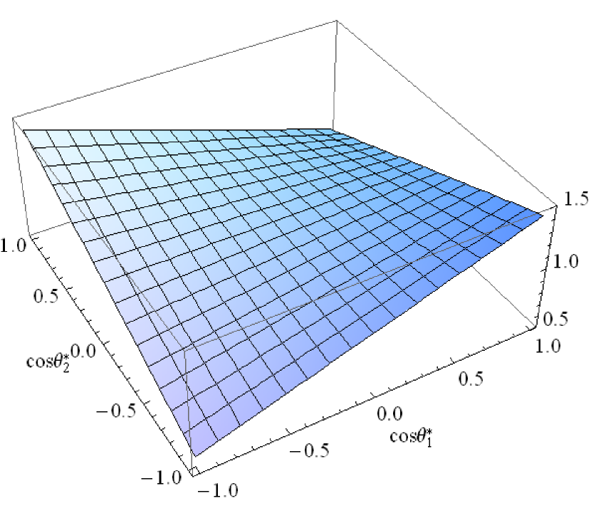
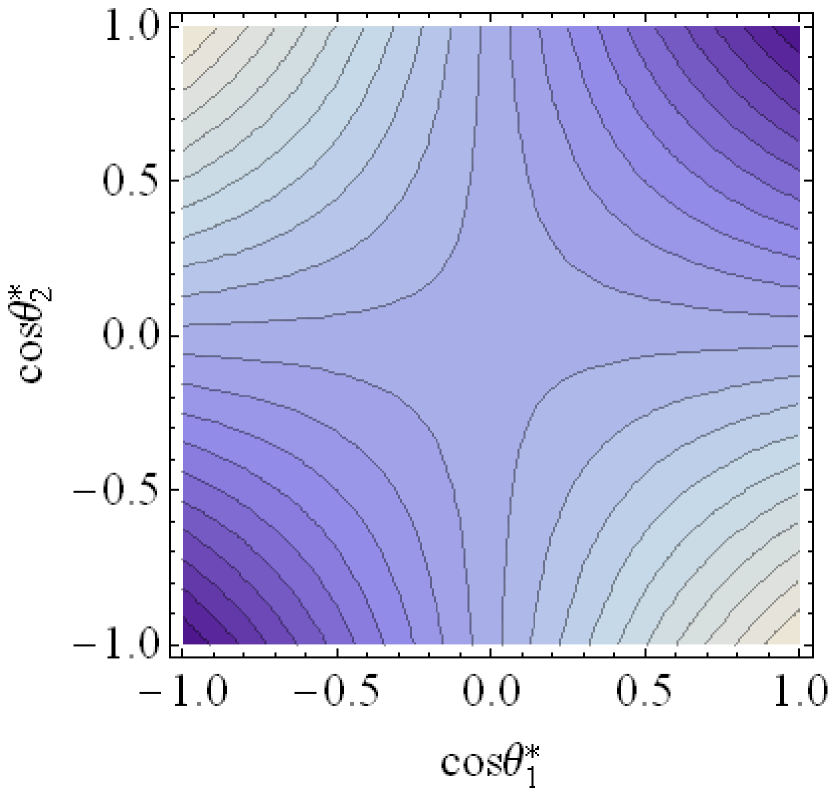
Figure 1: Correlation between $\cos{{\theta}^{*}_{1}}$ and $\cos{{\theta}^{*}_{2}}$ for a scalar or pseudo-scalar coupling.

2.2 Production via a Vector Coupling

As alternatives, we consider a couple of perturbative production mechanisms, namely the process ${\overline{q}}q\to{\overline{s}}s$ that is mediated by gluon exchange and hence via a vector coupling, or the process $gg\to{\overline{s}}s$ to which several perturbative diagrams contribute leading to a more complicated spin structure. In this subsection we consider the ${\overline{q}}q\to{\overline{s}}s$ case, initially assuming that the $s$ mass can be neglected.

In this case, there are only two combinations of the $s$ and ${\overline{s}}$ polarizations: either the polarization of the $s$ is along and that of the ${\overline{s}}$ is opposite to its momentum direction or the polarization of the $s$ is opposite and that of the ${\overline{s}}$ is along its momentum direction. When we consider the collision of unpolarized proton and proton or unpolarized lead-lead nuclei as in LHC, the cross sections for the above two combinations of the $s$ and ${\overline{s}}$ polarizations are the same. Hence we may add incoherently contributions of the form (2) with $P_{1}=+1,P_{2}=-1$ and with $P_{1}=-1,P_{2}=+1$, obtaining a correlation that is proportional to:

$${1\over 2}\Big{[}(1+a{\cos{\theta^{*}_{1}}})((1+a{\cos{\theta^{*}_{2}}})+(1-a{\cos{\theta^{*}_{1}}})((1-a{\cos{\theta^{*}_{2}}})\Big{]}=(1+a^{2}{\cos{\theta^{*}_{1}}}{\cos{\theta^{*}_{2}}})\ ,$$ (4)

where $a=0.642\pm 0.013$ [2]. Fig. 2 displays the between $\cos{{\theta}^{*}_{1}}$ and $\cos{{\theta}^{*}_{2}}$ to be expected on the basis of (4) in the case of a vector gluon coupling with $m_{s}=0$. We see that this is, in principle, easily distinguishable from the scalar/pseudoscalar case (3), thanks to the completely different $\Lambda{\overline{\Lambda}}$ polarization correlations and the strong analyzing power of $\Lambda\to p\pi^{-}$ decay.

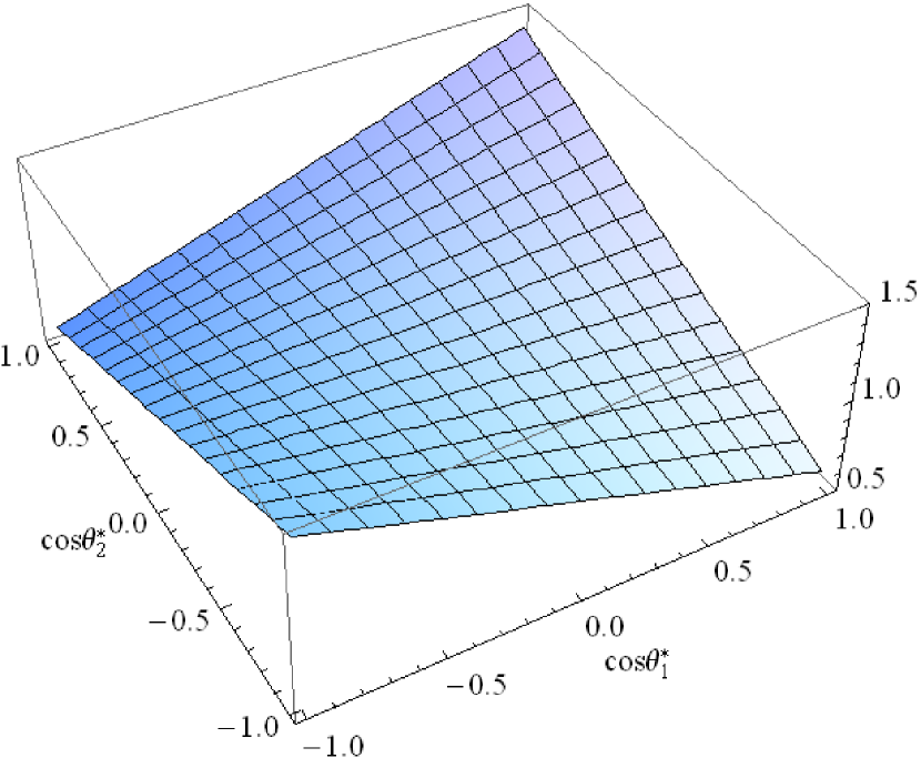
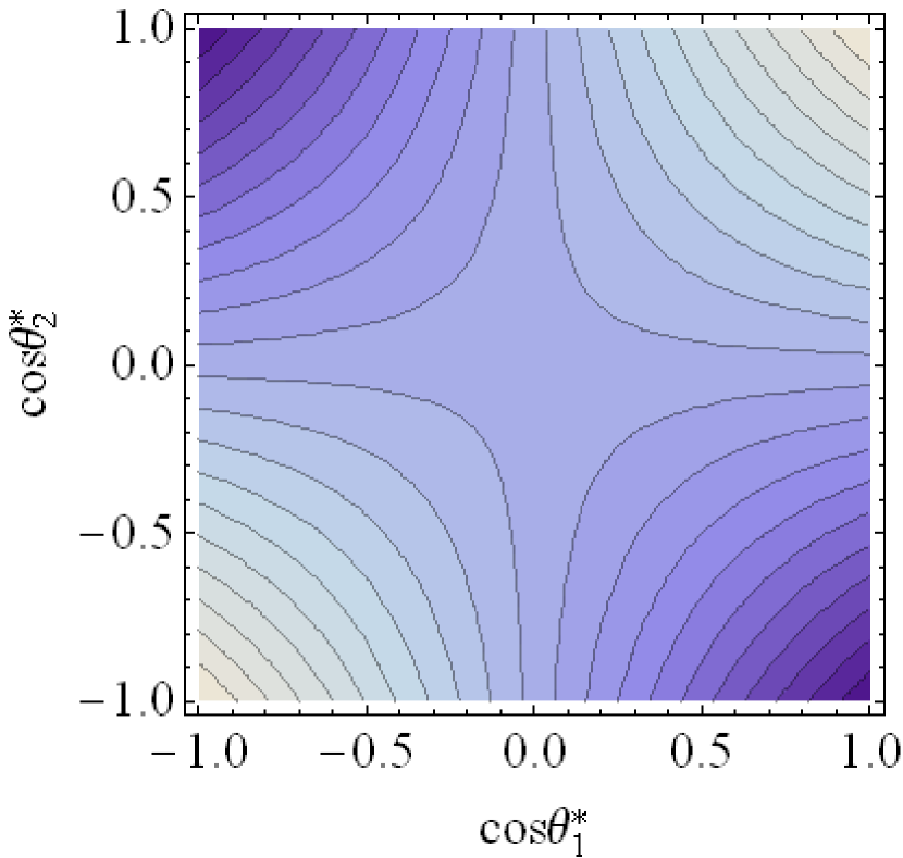
Figure 2: Correlation between $\cos{{\theta}^{*}_{1}}$ and $\cos{{\theta}^{*}_{2}}$ for a vector coupling when $m_{s}=0$.

The case $m_{s}\neq 0$ is slightly more complicated, with a non-trivial combination of $\Lambda{\overline{\Lambda}}$ polarization states becoming possible. An elementary calculation of ${\overline{q}}q\to{\overline{s}}s$, averaging over the polarizations of the massless quarks in the initial state and keeping track of the final-state polarizations, yields a decay-angle correlation that is proportional to:

$$\left[1+a^{2}{\cos{\theta^{*}_{1}}}{\cos{\theta^{*}_{2}}}\right]+\frac{x^{2}}{2}\left[1-a^{2}{\cos{\theta^{*}_{1}}}{\cos{\theta^{*}_{2}}}\right]\,,$$ (5)

where $a=0.642\pm 0.013$ is the $\Lambda$ decay parameter, as before, and $x\equiv 2m_{s}/\sqrt{s}$. This reduces to the case (4) in the limit $m_{s}\to 0$, but we see from the second term in (5) that the spin correlation in the massless case is diluted for $m_{s}\neq 0$, reflecting an admixture of the ³D₁ state. However, the spin correlation remains relatively large and of the same sign for all masses. As a measure of this, we define a one-dimensional correlation parameter $f(x)$ as follows:

$${(TR+BL)-(TL+BR)\over(TR+BL)+(TL+BR)}\ \equiv\ {a^{2}\over 4}\ f(x)\ =\ {a^{2}\over 4}\ {2-x^{2}\over 2+x^{2}}\ ,$$ (6)

where TR, BL, TL, and BR refer to the top-right, bottom-left, top-left and bottom-right quadrants, respectively, in the lower panels of Figs. 1 and 2, i.e., T $\equiv\cos{\theta^{*}_{2}}>0$, B $\equiv\cos{\theta^{*}_{2}}<0$, R $\equiv\cos{\theta^{*}_{1}}>0$ and L $\equiv\cos{\theta^{*}_{1}}<0$.

Graphs of the correlation function $f(x)$ for the different production mechanisms considered are shown in Fig. 3. We see that a clear distinction can be drawn between the scalar/pseudoscalar case, for which $f(x)=-1$ for all $x$, and the vector case, for which $1\geq f(x)\geq 1/3$. We return later to the $gg\to{\overline{s}}s$ case, which is shown as the intermediate line in Fig. 3.

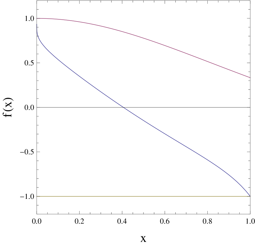
Figure 3: Graphs of the correlation $f(x)$ defined in (6) as a function of $x\equiv{2m_{s}\over{\sqrt{s}}}$, where $m_{s}$ is the strange quark mass. The topmost line is for the vector case (5), the lowest line is for the scalar and pseudoscalar cases (3), and the intermediate line is for the $gg\to{\overline{s}}s$ case $f_{gg}(x)$ given by (10).

2.3 Production via $gg$ Fusion

In this case there are three perturbative diagrams at lowest order: two ‘QED-like’ diagrams with $s$-quark exchanges in the $t$ and $u$ channels, and one distinctively non-Abelian diagram with direct $s$-channel gluon exchange. By itself, the latter would yield a vector coupling to ${\overline{s}}s$, akin to the previous ${\overline{q}}q$ case, but other couplings are made possible by the other diagrams, and become important if $m_{s}$ cannot be neglected. For example, if two gluons with the same helicity collide with $\sqrt{s}=2m_{s}$, they may produce an ${\overline{s}}s$ via an effective scalar or pseudoscalar coupling.

Although it is a trivial standard calculation [8] , for easy reference we include here the full squared amplitude for $gg\to{\overline{q}}q$ where $q$ is a generic massive quark, summed over final colours and averaged over initial colours and polarizations, in the form

$$\Sigma|{\cal M}|^{2}\ \;=\;\ {1\over 4}\ \pi^{2}{\alpha}_{S}^{2}\ ({\cal F}+\lambda{\cal G})\ ,$$ (7)

where $\lambda=-1$ when the polarizations of the $q$ and ${\overline{q}}$ are the same, $\lambda=+1$ when the polarizations of the $q$ and ${\overline{q}}$ are opposite, and we work in the centre-of-mass frame of the $gg$ and ${\overline{q}}q$ pairs. The coefficients ${\cal F}$ and ${\cal G}$ in (7) are given by

$${\cal F} = +\ {8\over 3}\ {E^{2}(E^{2}-p^{2}{\rm cos}^{2}\theta)+m^{2}E(E-p{\rm cos}\theta)-m^{4}\over E^{2}(E-p{\rm cos}\theta)^{2}}$$ (8)

$$+\ {8\over 3}\ {E^{2}(E^{2}-p^{2}{\rm cos}^{2}\theta)+m^{2}E(E+p{\rm cos}\theta)-m^{4}\over E^{2}(E+p{\rm cos}\theta)^{2}}$$

$$+\ (-{1\over 8})\times{16\over 3}\ {m^{2}p^{2}\over E^{2}(E-p{\rm cos}\theta)(E+p{\rm cos}\theta)}$$

$$+\ 3\ {(E^{2}-p^{2}{\rm cos}^{2}\theta)\over E^{2}}$$

$$-\ 3\ {E^{2}(E^{2}-p^{2}{\rm cos}^{2}\theta)-m^{2}Ep{\rm cos}\theta\over E^{3}(E-p{\rm cos}\theta)}$$

$$-\ 3\ {E^{2}(E^{2}-p^{2}{\rm cos}^{2}\theta)+m^{2}Ep{\rm cos}\theta\over E^{3}(E+p{\rm cos}\theta)}$$

and

$${\cal G} = +\ {8\over 3}\ {(-p^{4}+E^{4}{\rm cos}^{2}\theta-m^{2}Ep{\rm cos}\theta)\over E^{2}(E-p{\rm cos}\theta)^{2}}$$ (9)

$$+\ {8\over 3}\ {(-p^{4}+E^{4}{\rm cos}^{2}\theta+m^{2}Ep{\rm cos}\theta)\over E^{2}(E+p{\rm cos}\theta)^{2}}$$

$$+\ (-{1\over 8})\times{16\over 3}\ {m^{2}\Big{(}E^{2}(1-{\rm cos}^{2}\theta)+p^{2}\Big{)}\over E^{2}(E-p{\rm cos}\theta)(E+p{\rm cos}\theta)}$$

$$-\ 3\ {E^{2}(1-{\rm cos}^{2}\theta)-m^{2}{\rm cos}^{2}\theta\over E^{2}}$$

$$+\ 3\ {E^{4}(1-{\rm cos}^{2}\theta)+m^{2}Ep{\rm cos}\theta-m^{2}E^{2}{\rm cos}^{2}\theta\over E^{3}(E-p{\rm cos}\theta)}$$

$$+\ 3\ {E^{4}(1-{\rm cos}^{2}\theta)-m^{2}Ep{\rm cos}\theta-m^{2}E^{2}{\rm cos}^{2}\theta\over E^{3}(E+p{\rm cos}\theta)}\,,$$

where $E$, $p$, $m$ are the energy, magnitude of 3-momentum and mass of the final-state quark or antiquark, respectively, and $\theta$ is the angle between the 3-momentum of one of the initial gluons and that of final-state quark.

The correlation function $f(x)$ defined in (6) is given in this case by

$$f_{gg}(x)\;=\;\frac{({F}-{G})-({F}+{G})}{({F}-{G})+({F}+{G})}\;=\;-\,\,\frac{G}{F}\,,$$ (10)

where $F=\int_{-1}^{+1}d({\rm cos}\theta){\cal F}$ and $G=\int_{-1}^{+1}d({\rm cos}\theta){\cal G}$ with ${\cal F}$ and ${\cal G}$ given in (8) and (9), respectively. We note that ${\cal F}$ in (8) agrees with the formula presented in Ref. [9] for the spin-summed squared amplitude.

The sum of the first three terms in (8) and (9) is proportional to the formula for QED if we drop the relative color factor $(-{1\over 8})$ in their third terms. The value of $f_{gg}(x)=-\,{G}/{F}$ for $gg\to{\overline{s}}s$ is shown in Fig. 3 as a function of $x=2m_{s}/\sqrt{s}$. As expected, we see that the vector case $f\to 1$ is recovered in the massless limit $x\to 0$, whereas the scalar/pseudoscalar case $f\to-1$ is recovered in the non-relativistic limit $x\to 1$, and $f_{gg}$ interpolates monotonically between these limits for intermediate $x$ .

3 Summary and Discussion

We have pointed out that $\Lambda{\overline{\Lambda}}$ spin correlations offer, in principle, an interesting window into the hadronization process, as possible fossils of the spin correlations of their ancestral ${\overline{s}}s$ pairs. We have shown that $\Lambda{\overline{\Lambda}}$ pairs produced via perturbative vector couplings to ${\overline{s}}s$ could have very different spin correlations from those produced via non-perturbative scalar or pseudoscalar couplings to ${\overline{s}}s$. The spin correlations of $\Lambda{\overline{\Lambda}}$ pairs produced perturbatively via $gg$ collisions would be intermediate, tending towards the vector case if $m_{s}$ could be neglected, and towards the scalar/pseudoscalar case in the limit of non-relativistic ${\overline{s}}s$ pairs.

A detailed discussion of the experimental possibilities for measuring these correlations lies beyond the scope of this paper, but we emphasize that the ${\overline{s}}s$ production mechanisms might be quite different in different kinematic regimes. For example, ${\overline{s}}s$ pairs produced in high-$p_{T}$ jets might have a more ‘perturbative’ origin, whereas those produced in minimum-bias or heavy-ion collisions might have a more ‘non-perturbative’ origin. It would therefore be interesting to compare and contrast any $\Lambda{\overline{\Lambda}}$ spin correlations measured in these different conditions.

Superficial consideration of the LHC experiments suggests that ALICE [10] may be best suited for measurements of $\Lambda{\overline{\Lambda}}$ spin correlations in minimum bias and low-$p_{T}$ heavy-ion collisions, whereas ATLAS [11] and CMS [12] may be better suited for measurements at higher $p_{T}$. We emphasize that the $\Lambda{\overline{\Lambda}}$ pairs of interest are those with the lowest possible invariant mass, which are most likely to originate from the same ‘parent’ ${\overline{s}}s$ pair. Pairs with larger relative momenta are not expected to exhibit any significant spin correlations.

Acknowledgements

The work of J.E. is supported partly by the London Centre for Terauniverse Studies (LCTS), using funding from the European Research Council via the Advanced Investigator Grant 267352. The work of D.S.H. is supported partly by Korea Foundation for International Cooperation of Science & Technology (KICOS) and National Research Foundation of Korea (2011-0005226). D.S.H. thanks CERN for its hospitality while working on this subject. We thank Adam Jacholkowski for discussions of the experimental possibilities with ALICE, and Homer Neal and Daniel Scheirich for discussions of the experimental possibilities with ATLAS.

References

- [1] See, for example, J. R. Ellis, A. Kotzinian, D. Naumov and M. Sapozhnikov, Eur. Phys. J. C 52, 283 (2007) [arXiv:hep-ph/0702222], and references therein.
- [2] K. Nakamura et al. (Particle Data Group), J. Phys. G 37, 075021 (2010) and 2011 partial update for the 2012 edition.
- [3] See, for example, M. Burkardt and R. L. Jaffe, Phys. Rev. Lett. 70, 2537 (1993) [arXiv:hep-ph/9302232]; D. Ashery and H. J. Lipkin, Phys. Lett. B 469, 263 (1999) [arXiv:hep-ph/9908355]; B. Q. Ma, I. Schmidt, J. Soffer and J. J. Yang, Phys. Rev. D 64, 014017 (2001) [Erratum-ibid. D 64, 099901 (2001)] [arXiv:hep-ph/0103136].
- [4] See, for example, J.T. Jones et al. [WA21 Collaboration], Z. Phys. C 28, 23 (1987); S. Willocq et al. [WA59 Collaboration], Z. Phys. C 53, 207 (1992); D. deProspo et al. [E632 Collaboration], Phys. Rev. D 50, 6691 (1994); D. Buskulic et al. [ALEPH Collaboration], Phys. Lett. B 374, 319 (1996); K. Ackerstaff et al. [OPAL Collaboration], Eur. Phys. J. C 2, 49 (1998); P. Astier et al. [NOMAD Collaboration], Nucl. Phys. B 605, 3 (2001) [arXiv:hep-ex/0103047].
- [5] M. Gell-Mann, R. J. Oakes and B. Renner, Phys. Rev. 175, 2195 (1968).
- [6] Y. Nambu, Phys. Rev. Lett. 4, 380 (1960).
- [7] A. Bazavov et al., Phys. Rev. D 80, 014504 (2009) [arXiv:0903.4379 [hep-lat]].
- [8] G. Mahlon and S. Parke, Phys. Rev. D 53, 4886 (1996) and Phys. Rev. D 81, 074024 (2010), and references therein.
- [9] B.L. Combridge, Nucl. Phys. B 151, 429 (1979).
- [10] K. Aamodt et al. [ALICE Collaboration], JINST 3, S08002 (2008).
- [11] G. Aad et al. [ATLAS Collaboration], JINST 3, S08003 (2008).
- [12] S. Chatrchyan et al. [CMS Collaboration], JINST 3, S08004 (2008).