Mapping class groups of once-stabilized Heegaard splittings

Abstract.

We show that if a Heegaard splitting is the result of stabilizing a high distance Heegaard splitting exactly once then its mapping class group is finitely generated.

A Heegaard splitting for a compact, connected, closed, orientable 3-manifold $M$ is a triple $(\Sigma,H^{-},H^{+})$ where $\Sigma$ is a compact, separating surface in $M$ and $H^{-}$, $H^{+}$ are handlebodies in $M$ such that $M=H^{-}\cup H^{+}$ and $\partial H^{-}=\Sigma=H^{-}\cap H^{+}=\partial H^{+}$. The mapping class group $Mod(M,\Sigma)$ of the Heegaard splitting is the group of homeomorphisms $f:M\rightarrow M$ that take $\Sigma$ onto itself, modulo isotopies that fix $\Sigma$ setwise.

Heegaard splitings of distance greater than 3 are known to have finite mapping class groups [8] and certain distance two Heegaard splittings are known to have virtually cyclic mapping class groups [6]. By distance, we mean the distance $d(\Sigma)$ defined by Hempel [5], which we will review below. However, for stabilized (distance zero) Heegaard splittings, the problem of understanding their mapping class groups is much harder. Genus-two Heegaard splittings of the 3-sphere have finitely presented mapping class groups [1][4][12], but determining whether the mapping class groups of higher genus splittings of $S^{3}$ are finitely generated has proved to be a very difficult problem. We will study Heegaard splittings that results from stabilizing a high distance Heegaard splitting exactly once:

1 Theorem.

Let $(\Sigma^{\prime},H^{-}_{\Sigma^{\prime}},H^{+}_{\Sigma^{\prime}})$ be a Heegaard surface with genus $g$ and distance $d(\Sigma^{\prime})>2g+2$. If $(\Sigma,H^{-}_{\Sigma},H^{+}_{\Sigma})$ is the Heegaard splitting that results from stabilizing $\Sigma^{\prime}$ exactly once then $Mod(M,\Sigma)$ is finitely generated.

In fact, we will describe an explicit generating set in Section 1. Because every automorphism of $(M,\Sigma)$ is an automorphism of $M$, there is a canonical map $i:Mod(M,\Sigma)\rightarrow Mod(M)$. We will write $Isot(M,\Sigma)$ for the kernel of the map $i$, and will call this the isotopy subgroup. When $M$ is hyperbolic, $Isot(M,\Sigma)$ will be a finite index subgroup of $Mod(M,\Sigma)$.

To prove Theorem 1, we show that $Isot(M,\Sigma)$ is finitely generated in a very specific way. This will imply that $Mod(M,\Sigma)$ is finitely generated because $d(\Sigma^{\prime})>2g+2>3$, so $M$ must be hyperbolic, and $Isot(M,\Sigma)$ is finite index in $Mod(M,\Sigma)$. We will see that $Isot(M,\Sigma)$ is generated by two subgroups that have been recently classified by Scharlemann [13], with a well understood intersection. We conjecture that $Isot(M,\Sigma)$ is in fact a free product with amalgamation, but we are unable to prove this.

Note that every element in $Isot(M,\Sigma)$ is determined by an isotopy of $\Sigma$ in $M$, i.e. a continuous family of embedded surfaces $\{\Sigma_{r}\}$ such that $\Sigma_{0}=\Sigma_{1}=\Sigma$. The two subgroups that generate $Isot(M,\Sigma)$ will be defined as follows:

The stabilized Heegaard surface $\Sigma$ can be isotoped into either of the handlebodies $H^{\pm}_{\Sigma^{\prime}}$ bounded by the original Heegaard surface $\Sigma^{\prime}$. After such an isotopy it forms a Heegaard surface for the handlebody. Define $St^{-}(\Sigma)$ as the subgroup of $Isot(M,\Sigma)$ corresponding to isotopies entirely in $H^{-}_{\Sigma^{\prime}}$ and let $St^{+}(\Sigma)$ be the subgroup corresponding to isotopies in $H^{+}_{\Sigma^{\prime}}$.

These two subgroups are the isotopy subgroups of the mapping class groups for $\Sigma$, thought of as a Heegaard splitting for $H^{-}_{\Sigma^{\prime}}$ or $H^{+}_{\Sigma^{\prime}}$. Scharlemann [13] shows that such groups are finitely generated. We will show that $Isot(M,\Sigma)$ is generated by these two subgroups.

We review this generating set in Section 1, then determine a condition on isotopies of $\Sigma$ in $M$ that will guarantee that the corresponding element of $Isot(M,\Sigma)$ is generated by elements of $St^{-}(\Sigma)\cup St^{+}(\Sigma)$. The proof is based on the double sweep-out machinery developed by Cerf [2], Rubinstein-Scharlemann [11] and the author [7], which we review Sections 2 and 3. The proof of this Lemma and Theorem 1 are completed in Section 5.

1. Mapping class groups in handlebodies

A genus $g$ handlebody $H$ has, up to isotopy, a unique Heegaard splitting for each genus $h\geq g$ [14]. For $h=g$, this Heegaard splitting is a boundary parallel surface, which cuts $H$ into a genus $g$ handle-body and a trivial compression body $\partial H\times[0,1]$. The higher genus Heegaard splittings come from adding unknotted handles to the genus $g$ Heegaard splitting, as in Figure 1. This construction is called stabilization.

Figure 1. The genus $3$ Heegaard surface for a genus two handlebody.

An equivalent way to construct a genus $g+k$ Heegaard splitting of a handlebody $H$ is to take $k$ boundary parallel, properly embedded arcs $\alpha_{1},\dots,\alpha_{k}$ in $H$ and let $\Sigma$ be the boundary of a regular neighborhood of $\partial H\cup\alpha_{1}\cup\dots\cup\alpha_{k}$.

Let $\Sigma$ be the genus $g+1$ Heegaard splitting for $H$. Scharlemann [13] has determined a very simple generating set for the isotopy subgroup $Isot(H,\Sigma)$ in terms of the boundary parallel arc $\alpha\subset H$ that defines $\Sigma$. The surface $\Sigma$ bounds a genus $g+1$ handlebody on one side and a compression body with a single one-handle on the other side. There is exactly one non-separating compressing disk in the compression body, dual to the arc $\alpha$, so the isotopy subgroup of $\Sigma$ can be described entirely in terms of isotopies of $\alpha$.

Let $D\subset H$ be a disk whose boundary consists of the arc $\alpha$ and an arc in $\partial H$ (since $\alpha$ is unknotted) and let $E_{1},\dots,E_{g}$ be a collection of compressing disks for $\partial H$ that are disjoint from $D$ and cut $H$ into a single ball. By Theorem 1.1 in [13], $Isot(H,\Sigma)$ is generated by the following two subgroups. (We use slightly different notation here.)

1. Let $\mathfrak{F}(H,\Sigma)$ be the subgroup generated by isotoping the disk $D$ around $H$, and dragging $\alpha$ with it. Because $D\cap\partial H$ is an arc, each element is defined by a path in $\partial H$, modulo spinning around a regular neighborhood of $D\cap\partial H$. Thus this subgroup is isomorphic to an extension of $\pi_{1}(\partial H)$ by the integers.
   

2. Let $\mathfrak{A}(H,\Sigma)$ be the subgroup generated by fixing one endpoint of $\alpha$ and dragging the other around in the complement of a collection of properly embedded disks $D_{1},\dots,D_{g}$ whose complement in $H$ is a single ball. Because the complement of the disks is the ball, any path of one endpoint can be extended to an isotopy of $\alpha$ that ends back where it started. Any such mapping class is determined by an element of the fundamental group of the planar surface $\partial H\setminus(\bigcup D_{i})$, so this group is isomorphic to the fundamental group of the planar surface.
   

Figure 2. The isotopies that generate $\mathfrak{F}(H,\Sigma)$ and $\mathfrak{A}(H,\Sigma)$.

In particular, each of these subgroups is finitely generated, so $Isot(H,\Sigma)$ is finitely generated. Each of the subgroups $St^{\pm}(\Sigma)\subset Isot(M,\Sigma)$ is isomorphic to $Isot(H,\Sigma)$. Their intersection contains the subgroups $\mathfrak{F}(H^{\pm}_{\Sigma^{\prime}},\Sigma)$ in each handlebody because the isotopies defining these subgroups can be carried out within a regular neighborhood of the boundary.

We would like to show that if $\Sigma^{\prime}$ is a high distance Heegaard splitting then every element of $Isot(M,\Sigma)$ is a product of elements of $St^{-}(\Sigma)$ and $St^{+}(\Sigma)$. Fix spines $K^{-}$, $K^{+}$ of the handebodies $H^{-}_{\Sigma^{\prime}}$, $H^{+}_{\Sigma^{\prime}}$. The key will be the following Lemma:

2 Lemma.

Let $\{\Sigma_{r}|\ r\in[0,1]\}$ be an isotopy of the surface $\Sigma$ and assume there is a sequence of values $0=r_{0}<r_{1}<\dots<r_{k}=1$ with the property that for $r\in[r_{i},r_{i+1}]$, the surface $\Sigma_{r}$ is disjoint from $K^{-}$ when $i$ is even and disjoint from $K^{+}$ when $i$ is odd. Moreover, assume that each $\Sigma_{r_{i}}$ is a Heegaard surface for the complement of the two spines. Then the element of $Isot(M,\Sigma)$ defined by $\{\Sigma_{r}\}$ is generated by the elements of $St^{-}(\Sigma)\cup St^{+}(\Sigma)$.

Proof.

If every $\Sigma_{r}$ in the isotopy is disjoint from both spines $K^{\pm}$ then there is a value $\epsilon$ such that each $\Sigma_{r}$ is contained in $f^{-1}([\epsilon,1-\epsilon])$. This isotopy is conjugate to an isotopy in $H^{-}_{\Sigma^{\prime}}$ as well as to an isotopy in $H^{+}_{\Sigma^{\prime}}$, so it determines an element in the subgroup $St^{-}(\Sigma)\cap St^{+}(\Sigma)$.

If an isotopy $\{\Sigma_{r}\}$ ends with $\Sigma_{1}$ disjoint from both spines and isotopic to but not equal to $\Sigma$, then we can extend the isotopy so that $\Sigma_{1+\delta}=\Sigma$. This extension is not unique, but it is well defined up to multiplication by elements in $St^{-}(\Sigma)\cap St^{+}(\Sigma)$. Thus such an isotopy ending disjoint from $K^{-}\cup K^{+}$ determines a coset of the intersection.

If an isotopy is disjoint from $K^{+}$ and ends with the image of $\Sigma$ isotopic to a Heegaard surface for the complement of $K^{+}$ and $K^{-}$ then it can be extended to an isotopy that takes $\Sigma$ onto itself. Moreover, because the isotopy is disjoint from $K^{+}$, it is disjoint from the closure of some regular neighborhood $N$ of $K^{+}$ and $N$ is isotopic to $H^{+}(\Sigma^{\prime})$. Thus by conjugating the isotopy of $\Sigma$ with an ambient isotopy that takes $N$ onto $H^{+}(\Sigma^{\prime})$, we can turn the original isotopy into an isotopy of $\Sigma$ in $H^{-}_{\Sigma^{\prime}}$. Such an isotopy determines a coset of the intersection subgroup inside $St^{-}(\Sigma)$. Similarly, if the isotopy is disjoint from $K^{-}$, it determines a coset inside $St^{+}(\Sigma)$.

We have assumed that our isotopy $\{\Sigma_{r}\}$ can be cut into finitely many sub-intervals such that in each interval, $\Sigma_{r}$ is always disjoint from $K^{-}$ or always disjoint from $K^{+}$. The restriction of the isotopy $\{\Sigma_{r}\}$ to each interval determines a coset of $St^{-}(\Sigma)\cap St^{+}(\Sigma)$ in either $St^{-}(\Sigma)$ or $St^{+}(\Sigma)$. The element of $Isot(M,\Sigma)$ defined by the entire isotopy is a product of representatives for these cosets, and is thus in the subgroup generated by $St^{-}(\Sigma)\cup St^{+}(\Sigma)$. ∎

To prove Theorem 1, we must show that we can always find an isotopy of this form. The rest of the paper will be devoted to proving this:

3 Lemma.

If $d(\Sigma^{\prime})$ is greater than $2g+2$ then every element of $Isot(M,\Sigma)$ is represented by an isotopy satisfying the conditions of Lemma 2.

2. Sweep-outs and graphics

A sweep-out is a smooth function $f:M\rightarrow[-1,1]$ such that for each $t\in(-1,1)$, the level set $f^{-1}(t)$ is a closed surface. Moreover, $f^{-1}(-1)$ and $f^{-1}(1)$ is each a graph, called a spine of the sweep-out. The preimages $f^{-1}([-1,t])$ and $f^{-1}([t,1])$ are handlebodies for each $t\in(-1,1)$ so each level surface $f^{-1}(t)$ is a Heegaard surface for $M$ and the spines of the sweep-outs are spines of the two handlebodies in this Heegaard splitting. See [7] for a more detailed description of the methods described in this section.

We will say that a sweep-out represents a Heegaard splitting $(\Sigma^{\prime},H^{-}_{\Sigma^{\prime}},H^{+}_{\Sigma^{\prime}})$ if $f^{-1}(-1)$ is isotopic to a spine for $H^{-}_{\Sigma^{\prime}}$ and $f^{-1}(1)$ is isotopic to a spine for $H^{+}_{\Sigma^{\prime}}$. The level surfaces $f^{-1}(t)$ of such a sweep-out will be isotopic to $\Sigma^{\prime}$. Because the complement of the spines of a Heegaard splitting is a surface cross an interval, we can construct a sweep-out for any Heegaard splitting, i.e. we have the following:

4 Lemma.

Every Heegaard splitting of a compact, connected, closed orientable, smooth 3-manifold is represented by a sweep-out.

Given two sweep-outs, $f$ and $h$, their product is a smooth function $f\times h:M\rightarrow[-1,1]\times[-1,1]$. (That is, we define $(f\times h)(x)=(f(x),h(x))$.) The discriminant set for $f\times h$ is the set of points where the level sets of the two functions are tangent.

Generically, the discriminant set will be a one dimensional smooth submanifold in the complement in $M$ of the spines [9, 10]. The function $f\times h$ defines a piecewise smooth map from this collection of arcs and loops into the square $[-1,1]\times[-1,1]$. At the finitely many non-smooth points, the image is a cusp, which we will think of as a valence-two vertex. At the finitely many points where the restriction of $f$ is two-to-one, we see a crossing which we will think of as a valence-four vertex. There are also valence-one and -two vertices in the boundary of the square. The resulting graph is called the Rubinstein-Scharlemann graphic (or just the graphic for short). Kobayashi-Saeki’s approach [9] uses singularity theory to recover the machinery originally constructed by Rubinstein and Scharlemann in  [11] using Cerf theory [3].

5 Definition.

The function $f\times h$ is generic if the discriminant set is a smooth one-dimensional manifold and each arc $\{t\}\times[-1,1]$ or $[-1,1]\times\{s\}$ contains at most one vertex of the graphic.

Kobayashi and Saeki [9] have shown that after an isotopy of $f$ and $h$, we can assume that $f\times h$ is generic. The author has generalized this to an isotopy of sweep-outs as follows:

6 Lemma (Lemma 34 in [7]).

Every isotopy of the sweep-out $h$ is conjugate to an isotopy $\{h_{r}\}$ so that the graphic defined by $f$ and $h_{r}$ is generic for all but finitely many values of $r$. At the finitely many non-generic points, one of six changes can occur to the graphic, indicated in Figure 3:

1. A pair of cusps forming a bigon may cancel with each other of be created.

2. A pair of cusps adjacent to a common crossing may cancel or be created (similar to a Reidemeister one-move).

3. Three crossing may perform a Reidemeister three-move.

4. Two parallel edges may pinch together to form a pair of cusps, or vice versa.

5. Two edges may perform a Reidemeister two-move.

6. A cusp may pass across an edge.

Figure 3. Changes to the graphic under an isotopy of $f$.

For a more details description of these three moves, see [7].

3. Spanning and Splitting

Let $f$ and $h$ be sweep-outs. For each $s\in(-1,1)$, define $\Sigma_{s}=h^{-1}(s)$, $H^{-}_{s}=h^{-1}([-1,s])$ and $H^{+}_{s}=h^{-1}([s,1])$. Similarly, for $t\in(-1,1)$, define $\Sigma^{\prime}_{t}=f^{-1}(t)$. Following [7], we will say that $\Sigma^{\prime}_{t}$ is mostly above $\Sigma_{s}$ if each component of $\Sigma^{\prime}_{t}\cap H^{-}_{s}$ is contained in a disk subset of $\Sigma^{\prime}_{t}$. Similarly, $\Sigma^{\prime}_{t}$ is mostly below $\Sigma_{s}$ if each component of $\Sigma^{\prime}_{t}\cap H^{+}_{s}$ is contained in a disk in $\Sigma^{\prime}_{t}$.

Figure 4 shows the three possible positions for $\Sigma^{\prime}_{t}$ (shown in blue) with respect to $\Sigma_{s}$ for three different values of $s$ (outlined in red). For the highest value of $s$, $\Sigma^{\prime}_{t}$ is mostly below $\Sigma_{s}$. For the lowest value, it’s mostly above, and for the middle value (in which $\Sigma_{s}$ looks like a quadrilateral, $\Sigma^{\prime}_{t}$ is neither mostly above nor mostly below.

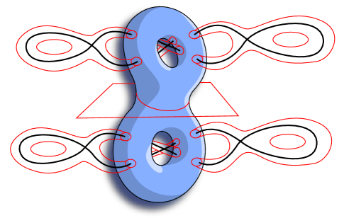
Figure 4. Changes to the graphic under an isotopy of $f$.

Let $R_{a}\subset(-1,1)\times(-1,1)$ be the set of all values $(t,s)$ such that $\Sigma^{\prime}_{t}$ is mostly above $\Sigma_{s}$. Let $R_{b}\subset(-1,1)\times(-1,1)$ be the set of all values $(t,s)$ such that $\Sigma^{\prime}_{t}$ is mostly below $\Sigma_{s}$. For any fixed $t\in(-1,1)$, there will be values $a,b$ such that $\Sigma^{\prime}_{t}$ will be mostly above $\Sigma_{s}$ if and only if $s\in[-1,a)$ and mostly above $\Sigma_{s}$ if and only if $s\in(b,1]$. In particular, both regions will be vertically convex.

As noted in [7], the closure of $R_{a}$ in $(-1,1)\times(-1,1)$ is bounded by arcs of the Rubinstein-Scharlemann graphic, as is the closure of $R_{b}$. The closures of $R_{a}$ and $R_{b}$ are disjoint (as long as the level surfaces of $f$ have genus at least two.)

7 Definition.

Given a generic pair $f$, $h$, we will say $h$ spans $f$ if there is a horizontal arc $[-1,1]\times\{s\}$ that intersects the interiors of both regions $R_{a}$ and $R_{b}$, as on the left side of Figure 5. Otherwise, we will say that $h$ splits $f$, as on the right of the figure.

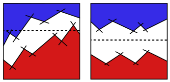
Figure 5. Spanning and splitting forms of the graphic.

Let $f$ be a sweep-out representing $(\Sigma^{\prime},H^{-}_{\Sigma^{\prime}},H^{+}_{\Sigma^{\prime}})$. By Lemma 16 in [7] we can choose a sweep-out $h$ for $(\Sigma,H^{-}_{\Sigma},H^{+}_{\Sigma})$ that spans $f$.

We can identify $\Sigma$ with any level surface of $h$ by an isotopy and we will choose a specific surface in a moment. For now, note that once we have chosen a level surface of $h$ to represent $\Sigma$, every element of $Isot(M,\Sigma)$ is represented by an isotopy of $\Sigma$, which can be extended to an ambient isotopy of $h$. By Lemma 6, we can choose the induced family of sweep-outs $\{h_{r}\}$ to be generic for all but finitely many values of $r$. At all these values, $h_{r}$ either spans or splits $f$. We will rule out splitting using the following Lemma:

8 Lemma (Lemma 27 in [7]).

If $h$ splits $f$ then $d(\Sigma^{\prime})$ is at most twice the genus of $\Sigma$.

Note that the notation here is slightly different than that used in [7]. In particular, the surfaces $\Sigma$ and $\Sigma^{\prime}$ play the opposite roles in [7] as they do here. In the statement of Theorem 1, we assume that $d(\Sigma^{\prime})$ is strictly greater than $2g+2$, so Lemma 8 implies that $h_{r}$ spans $f$ for every generic value of $r$. This will be the key to proving Lemma 3

4. Bicompressible surfaces in handlebodies

Recall that a two-sided surface $S\subset M$ is bicompressible if there are compressing disks for $S$ on both sides of the surface. We will say that $S$ is reducible if there is a sphere $P\subset M$ such that $P\cap S$ is a single loop that is essential in $S$. This term is usually used only for Heegaard surfaces, but we will apply it here to general bicompressible surfaces.

9 Lemma.

Let $F$ be a closed, orientable, genus $g$ surface and $S\subset(F\times[0,1])$ a closed, embedded, bicompressible surface of genus $g+1$ that separates $F\times\{0\}$ from $F\times\{1\}$. Then $S$ is reducible.

Proof.

Let $C^{-}$ be the closure of the component of $F\times[0,1]\setminus S$ adjacent to $F\times\{0\}$ and let $C^{+}$ be closure of the other component. Because $S$ is bicompressible, there are compressing disks $D^{-}\subset C^{-}$ and $D^{+}\subset C^{+}$ for $S$.

If $\partial D^{-}$ is non-separating in $S$ then compressing $S$ across $D^{-}$ produces a genus $g$ surface $S^{-}$ that separates $F\times\{0\}$ from $F\times\{1\}$. Because $F$ is also genus $g$, the surface $S^{-}$ must be isotopic to $F\times\{\frac{1}{2}\}$. In other words, $S^{-}$ separates $F\times[0,1]$ into two pieces homeomorphic to $F\times[0,1]$. If we reattach the tube to produce $S$ from $S^{-}$, we see that $C^{-}$ is a compression body that results from attaching a single one-handle to $F\times[0,1]$.

The same argument applies to $D^{+}$ and $C^{+}$. Thus if we can choose $D^{-}$ and $D^{+}$ to be non-separating, $S$ will be a genus $g+1$ Heegaard surface for $F\times[0,1]$. Every genus $g+1$ Heegaard surface for $F\times[0,1]$ is reducible by Scharlemann-Thompson’s classification of Heegaard splittings for surface-cross-intervals [15], so in this case we conclude that $S$ is reducible.

Otherwise, assume without loss of generality that every compressing disk for $S$ in $C^{-}$ is separating. If we compress $S$ along such a disk $D^{-}$ then the resulting surface $S^{-}$ consists of a genus $g$ component and a torus. As above, the genus $g$ component must be isotopic to $F\times\{\frac{1}{2}\}$ so that the torus component of $S^{-}$ is contained in $F\times[\frac{1}{2},1]$.

Because $F\times[\frac{1}{2},1]$ is atoroidal, the torus component $T$ $S^{-}$ can be compressed to form a sphere $T^{\prime}$. Because $F\times[\frac{1}{2},1]$ is irreducible, $T^{\prime}$ bounds a ball and we can recover $T$ by attaching a tube to $T^{\prime}$. Thus either bounds a solid torus or is contained in a ball (and bounds a knot complement), depending on which side of $T^{\prime}$ the tube us attached. In either case, $T$ has a (non-separating) compressing disk $D^{+}$. There is an arc $\alpha$ dual to the disk $D^{-}$ from the genus $g$ component of $S^{-}$ to $T$. Because $D^{-}$ and $D^{+}$ are on opposite sides of $S$, the arc most be adjacent to $T$ on the same side of the surface as the disk $D^{+}$. This is impossible if $T$ bounds a solid torus on the side containing $D^{+}$. Thus $T$ must be contained in a ball that intersects the arc $\alpha$ in a single point. This sphere will intersect $S$ in a single essential loop, so $S$ is reducible (though not necessarily a Heegaard surface). ∎

5. The Proof of Theorem 1

Proof of Lemma 3.

By assumption, $d(\Sigma^{\prime})>2g+2$ where $g$ is the genus of $\Sigma^{\prime}$. Because $\Sigma$ is a stabilization of $\Sigma^{\prime}$, its genus is $g+1$, so by Lemma 8, the graphic $f\times h_{r}$ can never be spanning. Thus there is a value $s_{r}$ for each sweep-out $h_{r}$ such that the horizontal line $[0,1]\times\{s_{r}\}$ passes through both regions $R_{a}$, $R_{b}$ of the graphic. Moreover, we can choose the values $s_{r}$ so that they vary continuously with $r$ and $s_{0}=s_{1}$. We will further choose values $a_{r}$, $b_{r}$ that vary continuously, except for finitely many jumps, such that $(a_{r},s_{r})\in R_{a}$ and $(b_{r},s_{r})\in R_{b}$. (A jump occurs when $a_{r}$ or $b_{r}$ is in a “tooth” of $R_{a}$ or $R_{b}$ that is moved away from the horizontal arc, as in Figure 6, and we choose a new point in a different tooth that still intersects the arc.)

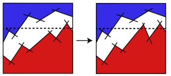
Figure 6. A jump in the value of $b_{r}$.

For each $r$, define $\Sigma_{r}=h^{-1}(s_{r})$. This family of surfaces defines an isotopy of $\Sigma$ corresponding to some element of $Isot(M,\Sigma)$. We will modify this isotopy so that at every time $r$, the surface is disjoint from one of the spines $K^{\pm}$ as follows:

The restriction of $f$ to $\Sigma_{r}$ is a Morse function on the surface, and the level sets at $a_{r}$ and $b_{r}$ form loops in this surface. In the level surface of $f$, these loops are trivial since $\Sigma$ is mostly above or mostly below $\Sigma^{\prime}$ at these points. Thus we can compress $\Sigma$ along these collections of loops to a surface that separates $K^{-}$ from $K^{+}$. Because $\Sigma$ has genus exactly one more than $\Sigma^{\prime}$, at most one of these loops can be an actual compression. For each $r$, this compression is either at $a_{r}$ or $b_{r}$.

At each of the finitely many values of $r$ where the values $a_{r}$ are discontinuous, let $a_{r}$ and $a^{\prime}_{r}$ be the left and right limits. If the level set at level $b_{r}$ contains an essential loop then the level sets at both levels $a_{r}$ and $a^{\prime}_{r}$ must be trivial, so neither defines a compression. If either of the level sets at $a_{r}$ or $a^{\prime}_{r}$ does contain a compression then $b_{r}$ does not. The same argument holds for a jump in $b_{r}$.

Thus we can cut the interval $[0,1]$ at points $0=r_{0}<r_{1}<\dots<r_{k}=1$ so that for $r\in[r_{i},r_{i+1}]$, the level sets at level $b_{r}$ are trivial when $i$ is even and the loops at level $a_{r}$ are trivial when $i$ is odd. Moreover, we can assume that for each even $i$, there is an $r\in[r_{i},r_{i+1}]$ such that the level loops of $a_{r}$ are non-trivial and vice-versa for odd $i$. In other words, we want to cut the interval into as few subintervals as possible.

For $r\in[r_{0},r_{1}]$, the level loops in $\Sigma_{r}$ at level $b_{r}$ are trivial in $\Sigma_{r}$. Each of these loops bounds a disk in each of the surfaces $\Sigma_{r}$, $\Sigma^{\prime}_{b_{r}}$ and there is, up to isotopy, a unique way to project the disk in $\Sigma_{r}$ onto the disk $\Sigma^{\prime}_{a_{r}}$, as in Figure 7. Let $S_{r}$ be the result of projecting all the disks in this way and assume we have chosen the projections to vary continuously with $r$ along the interval.

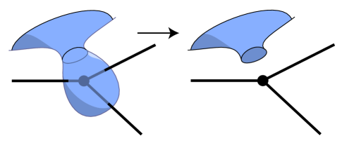
Figure 7. Removing trivial intersections between $\Sigma$ and a spine.

After the projection, the surface $S_{r}$ is entirely below level $b_{r}$ and is thus disjoint from $K^{+}$. For the intervals in which the level loops at level $a_{r}$ are trivial, $S_{r}$ will be disjoint from $K^{-}$. Repeat this construction for each $i$. The resulting isotopy defines the same element of $Mod(M,\Sigma)$ as the original isotopy, so all that remains is to show that $\Sigma_{r_{i}}$ is a Heegaard surface for the complement of both spines for each $i$.

We will start with $r_{1}$ and then repeat the argument for each $i$. By assumption, there is an $r\in[r_{0},r_{1}]$ such that the level set of $\Sigma_{r}$ at level $b_{r}$ is non-trivial. If we compress along all these loops, the resulting surface will contain a component isotopic to the boundary of a regular neighborhood of $K^{-}$, which is on the negative side of $\Sigma_{r}$. Thus at least one of the compressions must have been on the negative side of $\Sigma_{r}$.

Similarly, if we choose $r^{\prime}\in[r_{1},r_{2}]$, we can find a compressing disk on the positive side of $\Sigma_{r^{\prime}}$. If we choose $r$ to be the last such value and $r^{\prime}$ to be the first such value, then these compressing disks will determine compressing disks on both sides of $\Sigma_{r_{1}}$. Since $\Sigma_{r_{1}}$ is bicompressible, it is reducible by Lemma 9, as in Figure 8.

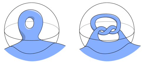
Figure 8. Two possible reducible surfaces in $M\setminus K^{+}$.

For each $r\in[r_{0},r_{1}]$, the surface $\Sigma_{r}$ is disjoint from $K^{-}$. The surfaces thus determine an isotopy of the surface inside the handlebody $M\setminus K^{+}$, so each $\Sigma_{r}$ is a Heegaard surface for this handlebody. Any reducing sphere for a Heegaard surface in an irreducible three-manifold determines a Heegaard surface for the ball bounded by the reducing sphere. In this case, we get a genus-one Heegaard surface, which is a standard unknotted torus [16]. Thus the reducing sphere for $\Sigma_{r_{1}}$, which is disjoint from both spines, bounds an unknotted handle, as on the left in Figure 8, and $\Sigma_{r_{1}}$ is a Heegaard surface for the complement of the two spines. By repeating this argument for each successive $i$, we complete the proof. ∎

Proof of Theorem 1.

Let $\gamma\in Isot(M,\Sigma)$ be an element of the isotopy subgroup of $\Sigma$, which is the result of stabilizing a Heegaard surface $\Sigma^{\prime}$ exactly once. Assume the distance $d(\Sigma^{\prime})$ is strictly greater than $2g+2$. Then by Lemma 3, we can represent $\gamma$ by an isotopy satisfying the conditions of Lemma 2. Then by Lemma 2, $\gamma$ is in the subgroup generated by $St^{-}(\Sigma)\cup St^{+}(\Sigma)\subset Isot(M,\Sigma)$.

Since $\gamma$ was an arbitrary element, $St^{-}(\Sigma)\cup St^{+}(\Sigma)$ must generate the entire group $Isot(M,\Sigma)$. Because $d(\Sigma)>2g+2>3$, $M$ is hyperbolic by Hempel’s Theorem [5] (and geometrization). Thus $Mod(M)$ is finite, so $Isot(M,\Sigma)$ is a finite index subgroup of $Mod(M,\Sigma)$. Since a finite index subgroup of $Mod(M,\Sigma)$ is finitely generated, the entire group is finitely generated. ∎

References

- [1] Erol Akbas, A presentation for the automorphisms of the 3-sphere that preserve a genus two Heegaard splitting, Pacific J. Math. 236 (2008), no. 2, 201–222. MR 2407105 (2009d:57029)
- [2] Jean Cerf, Sur les difféomorphismes de la sphère de dimension trois , Lecture Notes in Mathematics, No. 53, Springer-Verlag, Berlin, 1968. MR 0229250 (37 #4824)
- [3] by same author, La stratefacation naturelle des especes de fonctions differentiables reeles et la theoreme de la isotopie., Publ. Math. I.H.E.S. 39 (1970).
- [4] Sangbum Cho, Homeomorphisms of the 3-sphere that preserve a Heegaard splitting of genus two, Proc. Amer. Math. Soc. 136 (2008), no. 3, 1113–1123 (electronic). MR 2361888 (2009c:57029)
- [5] John Hempel, 3-manifolds as viewed from the curve complex, Topology 40 (2001), no. 3, 631–657. MR 1838999 (2002f:57044)
- [6] Jesse Johnson, Heegaard splittings and open books, in preparation.
- [7] by same author, Bounding the stable genera of Heegaard splittings from below, J. Topol. 3 (2010), no. 3, 668–690. MR 2684516
- [8] by same author, Mapping class groups of medium distance Heegaard splittings, Proc. Amer. Math. Soc. 138 (2010), no. 12, 4529–4535. MR 2680077
- [9] Tsuyoshi Kobayashi and Osamu Saeki, The Rubinstein-Scharlemann graphic of a 3-manifold as the discriminant set of a stable map, Pacific J. Math. 195 (2000), no. 1, 101–156. MR 1781617 (2001i:57026)
- [10] J. Mather, Stability of mappings V., Advances in Mathematics 4 (1970), no. 3, 301–336.
- [11] Hyam Rubinstein and Martin Scharlemann, Comparing Heegaard splittings—the bounded case, Trans. Amer. Math. Soc. 350 (1998), no. 2, 689–715. MR 1401528 (98d:57033)
- [12] Martin Scharlemann, Automorphisms of the 3-sphere that preserve a genus two Heegaard splitting, Bol. Soc. Mat. Mexicana (3) 10 (2004), no. Special Issue, 503–514. MR 2199366 (2007c:57020)
- [13] by same author, Generating the genus g+1 Goeritz group of a genus g handlebody, preprint (2011), arXiv:1108.4671.
- [14] Martin Scharlemann and Abigail Thompson, Heegaard splittings of are standard, Math. Ann. 295 (1993), no. 3, 549–564. MR 1204837 (94b:57020)
- [15] by same author, Heegaard splittings of are standard, Math. Ann. 295 (1993), no. 3, 549–564. MR 1204837 (94b:57020)
- [16] Friedhelm Waldhausen, Heegaard-Zerlegungen der -Sphäre, Topology 7 (1968), 195–203. MR 0227992 (37 #3576)