Quantum Coherent Dynamics at Ambient Temperature in Photosynthetic Molecules

Abstract

Photosynthetic antenna complexes are responsible for absorbing energy from sunlight and transmitting it to remote locations where it can be stored. Recent experiments have found that this process involves long-lived quantum coherence between pigment molecules, called chromophores, which make up these complexes Expected to decay within 100 fs at room temperature, these coherences were instead found to persist for picosecond time scales, despite having no apparent isolation from the thermal environment of the cell. This paper derives a quantum master equation which describes the coherent evolution of a system in strong contact with a thermal environment. Conditions necessary for long coherence lifetimes are identified, and the role of coherence in efficient energy transport is illuminated. Static spectra and exciton transfer rates for the PE545 complex of the cryptophyte algae CS24 are calculated and shown to have good agreement with experiment.

When a solar photon is captured by a photosynthetic organism, it creates a localized excited state, or exciton, in one of several optically active pigment molecules, or chromophores, in a specialized antenna complex. The exciton is then conveyed via electrostatic coupling to a remote reaction center where its energy can be stored and ultimately used to do work. Because the exciton has a natural lifetime on the order of nanoseconds, it is necessary that the transfer process be very rapid, so that the exciton’s energy can be stored before it decays.

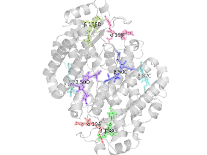
Figure 1: Spatial arrangement of chromophores and protein backbone in PE545.

In order to understand the dynamics of photosynthesis, it is necessary to understand the dynamics of the exciton transfer process. However, such an understanding is complicated by the many internal degrees of freedom in the chromophores, and by interactions between the chromophore and the cellular environment. In the limit of weak coupling between chromophores, Förster theory beljonne2009beyond describes the transfer of excitons as a fully incoherent process. In the opposite limit, of weak coupling between chromophores and the surrounding environment, Redfield theory ishizaki2009adequacy describes the coherent transport of excitons using a perturbative expansion over a weak system-reservoir coupling, but may give unphysical negative or diverging exciton populations. Such unphysical behavior may be avoided through use of a secular approximation may2004charge , at the cost of decoupling the evolution of populations and coherences. Neither the Förster nor the Redfield limits is applicable to the limit in which the coupling between chromophores and between chromophores and the environment are both strong.

Nonperturbative approaches to the problem of exciton dynamics are less easily classified. The Haken, Reineker, Strobl modelhaken1973exactly ; capek1985generalized calculates the evolution of an electronic reduced density matrix due to electrostatic couplings between chromophores, with dephasing due to interaction with the environment. This model predicts long lived coherences between chromophores, but yields an equilibrium state with equal occupation probabilities for all chromophores, which is true only in the high temperature limit. Other approaches include the stochastic Schrödinger equation diósi1997non ; strunz1996linear and methods based on quantum walksmohseni2008environment . Several studies have found that interplay between the system and the environment, including nonmarkovian effects and details of the system’s vibrational structure, can affect coherence lifetimes and the rates of exciton transfer rebentrost2009environment ; caruso2009 .

The need for an improved treatment of exciton dynamics has been highlighted by the recent observation of long lived coherences between chromophores in photosynthetic antenna complexes lee2007coherence ; collini2010coherently ; gregory2007evidence ; savikhin1997oscillating . Whereas a simple energy-time uncertainty approach would suggest that such coherences must die in less than 100 fs van2010quantum , they were instead found to persist for picosecond timescales – on the order of the time needed for excitons to travel between chromophores. Rather than being confined to the low temperature limit, such lifetimes were observed even at room temperature, shedding doubt on the common assumption that biological systems are too ”hot and wet” to display quantum coherent behavior sarovar2010quantum .

The observation of long lived coherences in biological systems at room temperature raises several questions. First, how can these coherences persist in the thermal environment of the cell? Are the coherences somehow protected from interaction with the outside world, or are they preserved through another mechanism? Second, can the organism exploit coherence to improve the efficiency of photosynthesis? Does coherent transport alter the rate at which excitons travel between chromophores? Does the quantum information contained in the coherence terms affect the flow of population through the complex? Some have speculated that the complex may perform quantum information processing to optimize the transfer path gregory2007evidence , although others hoyer2010limits ; rebentrost2009environment have found that such speedup may be short lived. In addition to these questions, the underlying problem of a few state system with internal degrees of freedom interacting with a thermal reservoir may have applications in fields such as quantum computing, where loss of coherence due to interactions with the surrounding environment is a major limiting factor unruh1995maintaining .

This paper presents a new theory of coherent evolution in a multichromophore system which does not rely on a perturbative parameter. Instead, an assumption of rapid thermalization of vibrational degrees of freedom is used to derive equations of motion for a slowly evolving electronic reduced density matrix. In this way, both the transfer of exciton population and the evolution of coherences are treated on an equal footing. The resulting theory gives a simple explanation for long coherence lifetimes in the high temperature limit for a system which interacts strongly with its environment.

Section I derives equations of motion for an electronic reduced density matrix. Part I.3 reduces the full electronic + vibrational+environment density matrix to yield equations of motion for a reduced electronic density matrix, while part I.4 reduces these equations of motion to the form of the Haken Reineker Strobl model haken1973exactly , in which both the density matrix and the effective coupling incorporate thermodynamic quantities. Section II applies the resulting theory to a two chromophore system, to find lifetimes for the decay of coherence or the transfer of population between two chromophores. Section III applies this theory to the PE545 antenna complex of cryptophyte algae Rhodomonas CS24, shown in Figure 1, comparing to experimentally measured transfer times, as well as absorption, circular dichroism and fluorescence spectra.

I Equations of motion

Although the primary function of an antenna complex is to transfer electronic excitation between chromophores, it is not a purely electronic system in the sense of having electronic degrees of freedom which can be separated from the other degrees of freedom in the system. Rather, both the ground and excited ”states” of a particular chromophore correspond to an infinite number of vibronic states. Each of these vibronic states may interact with the local environment of the cell, a system which is complicated and difficult to characterize. In order to calculate equations of motion for the purely electronic quantity of interest, it is necessary to remove the vibrational and environmental information from the system – ie, to reduce the full electronic + vibrational + environmental density matrix to a purely electronic reduced density matrix.

I.1 The Vibrational/Electronic System

The full electronic + vibrational + environmental Hamiltonian may be partitioned into an electronic + vibrational system interacting with a reservoir, $H=H_{S}+H_{R}+H_{SR}$. Here the part of the total Hamiltonian dealing with the system is relatively well characterized, while that dealing with the reservoir is less so. To aid in the reduction to a purely electronic density matrix, it is useful to write vibronic states as the product of vibrational and electronic eigenstates. Writing the system Hamiltonian $H_{S}=H^{\text{el}}_{0}+H^{\text{vib}}_{0}+V$, system eigenstates in the single exciton manifold can be written $\mathinner{|{i,\vec{n}}\rangle}$, where $i$ is the excited chromophore and $\vec{n}$ the vector of excited vibrational states, $\vec{n}=n_{1},n_{2},n_{3}\dots$. In this basis, $H^{\text{el}}_{0}\mathinner{|{i,n}\rangle}=E_{i}\mathinner{|{i,n}\rangle}$, $H^{\text{vib}}_{0}\mathinner{|{i,n_{i}}\rangle}=\epsilon^{(i)}_{n}\mathinner{|{i,n_{i}}\rangle}$ and $\epsilon^{(i)}_{\vec{n}}=\sum_{j}\epsilon^{(i)}_{n_{j}}$. Vibrational states of the excited chromophore $\mathinner{|{i,n_{i}}\rangle}$ may differ from those of the unexcited chromophore $\mathinner{|{0,n_{i}}\rangle}$ due to differing potential energy surfaces. Here it is convenient to introduce electronic $\mu^{+}_{i}=\mathinner{|{i}\rangle}\mathinner{\langle{0}|}$ and vibrational $\nu^{+}_{n_{i}}=\mathinner{|{i,n_{i}}\rangle}\mathinner{\langle{i,0_{i}}|}+\mathinner{|{0,n_{i}}\rangle}\mathinner{\langle{0,0_{i}}|}$ excitation operators, so that the state of the complex can be written as the product of excitation operators acting on an initial ground state

$$\psi=\sum_{i,\vec{n}}(\prod_{j}b^{j}_{m}\nu^{+}_{m_{j}})a_{i}\mu^{+}_{i}\mathinner{|{0}\rangle}.$$ (1)

Deexcitation operators $\mu_{i}$ and $\nu_{n_{i}}$ are given by the Hermitian conjugates of the excitation operators. In the limit that electronically exciting one chromophore does not affect the potential energy surfaces on other chromophores, the electronic excitation/deexcitation operators commute with the vibrational excitation/deexcitation operators for a different chromophore.

I.2 The reservoir

In contrast to the system being studied, whose Hamiltonian is relatively well known and studied, the reservoir may be complicated and difficult to characterize. In Förster theory, rapid dephasing of electronic and vibrational degrees of freedom allow explicit consideration of the reservoir to be avoided, as dynamics can be calculated from the overlap of the donor emission and the acceptor absorption spectra scholes2003long . In Redfield theory, the reservoir is often modeled as an infinite set of harmonic oscillators breuer2002theory .

In the current work, each chromophore is assumed to interact with a separate reservoir, so that $H_{SR}$ can be written as $H_{SR}=\sum_{i}V^{(i)}_{SR}\mathinner{|{i}\rangle}\mathinner{\langle{i}|}$, and the system-reservoir interaction is incapable of transferring excitation between chromophores. As in Förster theory, an assumption of rapid thermalization allows electronic equations of motion to be derived without explicit reference to the form of $V^{(i)}_{SR}$.

If eigenstates of the reservoir Hamiltonian corresponding to chromophore $i$ are given by $H^{(i)}_{R}\mathinner{|{\zeta_{i}}\rangle}=E_{\zeta_{i}}\mathinner{|{\zeta_{i}}\rangle}$, then the mixing of eigenstates $\mathinner{|{i,\vec{n},\zeta_{i}}\rangle}$ is governed by $V$ and $H_{SR}$. The assumption of rapid thermalization is that the short time evolution of the system is given by $U(t,t_{0})\approx\prod_{i}U^{(i)}(t,t_{0})$, where $U^{(i)}(t,t_{0})=\exp[-i\int_{t_{0}}^{t}V^{(i)}_{SR}(\tau)d\tau]\mathinner{|{i}\rangle}\mathinner{\langle{i}|}$. If $\psi(t)=\sum_{i,\vec{n},\zeta_{i}}a_{i}(t)b^{(i)}_{\vec{n}}(t)c_{\zeta_{i}}(t)\mathinner{|{i,\vec{n},\zeta_{i}}\rangle}$, the electronically diagonal character of $U$ means that $a_{i}(t)$ does not evolve, while the vibrational and environmental degrees of freedom are driven to thermal equilibrium

$$\text{Tr}_{\zeta_{i}=\zeta^{\prime}_{i}}b^{(i)}_{n}b^{*(i)}_{n^{\prime}}c^{(i)}_{\zeta_{i}}c^{*(i)}_{\zeta^{\prime}_{i}}=\delta_{n,n^{\prime}}P^{(i)}_{n}.$$ (2)

Here $P^{(i)}_{n}$ is the probability of vibrational state $n$ on chromophore $i$ being excited, while $P^{(i)}_{\vec{n}}=\prod_{j}P^{(i)}_{n_{j}}$ is the probability of a particular vector of vibrational states being excited.

Eq. 2 can now be used to reduce equations of motion for the full electronic + vibrational+environment system to a purely electronic subsystem.

I.3 Density Matrix Reduction

Electronic equations of motion can be found by tracing over environmental and vibrational degrees of freedom. To this end, let

$$\begin{split}\rho_{i\vec{n}\zeta j\vec{m}\eta}=a_{i}b_{\vec{n}}c_{\zeta_{i}}\mathinner{|{i,\vec{n},\zeta_{i}}\rangle}\mathinner{\langle{j,\vec{m},\eta_{j}}|}a^{*}_{j}b^{*}_{\vec{m}}c^{*}_{\eta_{j}}\times\\ e^{-i(E_{i}+\epsilon^{i}_{\vec{n}}+E_{\zeta_{i}}-E_{j}-\epsilon^{(j)}_{\vec{m}}-E_{\eta_{j}})t},\end{split}$$ (3)

be the full density matrix written with factorized coeffients and

$$\sigma_{i\vec{n}\zeta_{i}j\vec{m}\eta_{j}}=c^{*}_{\zeta^{\prime}_{i}}\mathinner{|{\zeta^{\prime}_{i}}\rangle}\mathinner{\langle{\zeta^{\prime}_{i}}|}(\prod_{n^{\prime}_{j}}b^{*}_{n^{\prime}_{j}}\mathinner{|{n^{\prime}_{j}}\rangle}\mathinner{\langle{n^{\prime}_{j}}|})\rho_{i\vec{n}\vec{\zeta}j\vec{m}\vec{\eta}}(\prod_{m^{\prime}_{j}}b_{m^{\prime}_{j}}\mathinner{|{m^{\prime}_{j}}\rangle}\mathinner{\langle{m^{\prime}_{j}}|})c_{\eta^{\prime}_{i}}\mathinner{|{\eta^{\prime}_{j}}\rangle}\mathinner{\langle{\eta^{\prime}_{j}}|}$$ (4)

be an auxiliary matrix defined in terms of the squares of vibrational and environmental coefficients, so that $a_{i}a^{*}_{j}=\sum_{\vec{n},\vec{m},\zeta_{i},\eta_{j}}\sigma_{i\vec{n}\zeta_{i}j\vec{m}\eta_{j}}$. Equations of motion for the electronic coefficients $a_{i}a^{*}_{j}$ can now be found by substituting Eq. 2 into equations of motion for $\sigma$.

The rate of dephasing between different chromophores is found by substituting Eq. 2 into Eq. 4, yielding

$$a_{i}a^{*}_{j}(t)=a_{i}a^{*}_{j}(0)\sum_{\vec{n},\vec{m}}P^{(i)}_{\vec{n}}P^{(j)}_{\vec{m}}e^{-i(E_{i}+\epsilon^{(i)}_{\vec{n}}-E_{j}-\epsilon^{(j)}_{\vec{m}})t},$$ (5)

Similarly, equations of motion for coherent evolution are found by substituting Eq. 2 into the operator equation of motion for $\sigma$ due to $H_{S}+H_{R}$, $\frac{\partial}{\partial t}\sigma=-i[H_{S}+H_{R},\sigma]$, yielding

$$\begin{split}\frac{\partial}{\partial t}a_{i}a^{*}_{j}=-i[V_{i\vec{n}k\vec{p}}P^{(k)}_{\vec{p}}P^{(j)}_{\vec{m}}a_{k}a^{*}_{j}e^{-i(E_{i}+\epsilon^{(i)}_{\vec{n}}-E_{k}-\epsilon^{(k)}_{\vec{p}})t}-\\ a_{i}a^{*}_{k}P^{(i)}_{\vec{n}}P^{(k)}_{\vec{p}}V_{k\vec{p}j\vec{m}}e^{-i(E_{k}+\epsilon^{(k)}_{\vec{p}}-E_{j}-\epsilon^{(j)}_{\vec{m}})t}],\end{split}$$ (6)

where $V_{k\vec{p}j\vec{m}}=\mathinner{\langle{0}|}\mu_{i}\nu_{\vec{n}}V\nu^{+}_{\vec{m}}\mu^{+}_{j}\mathinner{|{0}\rangle}$.

The complicated forms of Eqs. 5 and 6, which result in part from their generality, may be simplified by making assumptions about the vibrational spectrum and the form of the vibrational/electronic operator $V$. In terms of the vibrational density of states

$$D^{(i)}(\epsilon)=\sum_{\vec{n}}\delta(\epsilon-\epsilon^{(i)}_{\vec{n}})$$ (7)

and thermodynamic weighting factor

$$P^{(i)}(\epsilon)=P^{(i)}_{\vec{n}}|_{\epsilon=\epsilon^{(i)}_{\vec{n}}},$$ (8)

the dephasing between two chromophores given in Eq. 5 becomes

$$\begin{split}a_{i}a^{*}_{j}(t)=a_{i}a^{*}_{j}(0)\int d\epsilon\int d\epsilon^{\prime}P^{(i)}(\epsilon)D^{(i)}(\epsilon)P^{(j)}(\epsilon^{\prime})D^{(j)}(\epsilon^{\prime})\times\\ e^{-i(E_{i}+\epsilon-E_{j}-\epsilon^{\prime})t}.\end{split}$$ (9)

while for $i=j$, unitarity of $U^{(i)}(t,t_{0})$ ensures that $a_{i}a^{*}_{i}(t)=a_{i}a^{*}_{i}(0)$.

If the vibronic term $V$ is assumed to be purely electronic, so that $V=\sum_{ij}V_{ij}\mu^{+}_{i}\mu_{j}$, then

$$V_{i\vec{n}j\vec{m}}=V_{ij}\mathinner{\langle{0}|}\mu_{i}\nu_{n_{i}}\mu^{+}_{i}\nu^{+}_{m_{i}}\mathinner{|{0}\rangle}\mathinner{\langle{0}|}\nu_{n_{j}}\mu_{j}\nu^{+}_{m_{j}}\mu^{+}_{j}\mathinner{|{0}\rangle}\prod_{k\neq i,j}\delta_{n_{k},m_{k}}.$$ (10)

where the matrix elements are Franck-Condon overlaps between vibrational states of the excited and unexcited chromophores.

Further simplification can be achieved by replacing the oscillatory integrals in Eq. 6 with their average over some period $\Delta t$. As $\Delta t$ grows, this average goes to 1 if the energies in the exponential sum to 0; 0 otherwise. Including the effects of Lorentzian dephasing between chromophores in this average yields an exponential linewidth, so that

$$\frac{1}{\Delta t}\int dte^{-i(E_{i}+\epsilon^{(i)}_{\vec{n}}-E_{k}-\epsilon^{(k)}_{\vec{p}})t}\frac{\beta^{2}}{\beta^{2}+t^{2}}\propto e^{-2\beta|E_{i}+\epsilon^{(i)}_{\vec{n}}-E_{k}-\epsilon^{(k)}_{\vec{p}}|}.$$ (11)

Eq. 6 then becomes

$$\frac{\partial}{\partial t}(a_{i}a^{*}_{j})=-iV_{ik}T_{k\rightarrow i}(a_{k}a^{*}_{j})+i(a_{i}a^{*}_{k})V_{kj}T_{k\rightarrow j}$$ (12)

where

$$\begin{split}T_{i\rightarrow j}=\int d\epsilon\int d\epsilon^{\prime}&D^{(i)}(\epsilon)D^{(j)}(\epsilon^{\prime})\\ &P^{(i)}(\epsilon)\mathbb{F}(\epsilon,\epsilon^{\prime})\mathbb{L}(E_{i}+\epsilon-E_{j}-\epsilon^{\prime}),\end{split}$$ (13)

$$\mathbb{F}(\epsilon,\epsilon^{\prime})=\mathinner{\langle{0}|}\mu_{i}\nu_{n_{i}}\mu^{+}_{i}\nu^{+}_{m_{i}}\mathinner{|{0}\rangle}\mathinner{\langle{0}|}\nu_{n_{j}}\mu_{j}\nu^{+}_{m_{j}}\mu^{+}_{j}\mathinner{|{0}\rangle}|_{\epsilon=\epsilon^{(i)}_{n},\epsilon^{\prime}=\epsilon^{(j)}_{m}}$$ (14)

is the Franck Condon overlap and $\mathbb{L}(\Delta E)$ is the linewidth.

I.4 The thermalized density matrix

In Eq. 12, $T_{i\rightarrow j}$ plays the role of the overlap between donor emission and acceptor absorption spectra in Förster theory: it reflects the number of acceptor states sufficiently close in energy to an occupied donor state to receive population. The asymmetry of $T_{i\rightarrow j}$ reflects irreversible flow of population from high- to low energy chromophores: for $E_{i}>E_{j}$, every potential donor state on chromophore $i$ has a degenerate acceptor state on chromophore $j$, while the reverse is true only if $\epsilon^{(j)}\geq E_{i}-E_{j}$.

The asymmetric form of Eq. 12 which results from this irreversible flow can be rectified by defining a symmetrized density matrix $\tilde{\rho}_{ij}\equiv e^{\alpha_{i}+\alpha_{j}}a_{i}a^{*}_{j}$ and effective coupling $\tilde{V}_{ij}=V_{ij}T_{i\rightarrow j}e^{\gamma_{i}-\gamma_{j}}$. Requiring that the effective coupling be Hermitian yields $\frac{T_{i\rightarrow j}}{T_{j\rightarrow i}}=e^{2\gamma_{i}-2\gamma_{j}}$, while requiring that Eq. 12 be unaffected by the change of variables requires that $\alpha_{i}=-\gamma_{i}$. Performing this symmetrization and approximating the dephasing between chromophores as exponential yields a master equation of the form

$$\frac{\partial}{\partial t}\tilde{\rho}=-i[\tilde{V},\tilde{\rho}]-(1-\delta_{ij})\Gamma\tilde{\rho}.$$ (15)

For a constant density of states and Boltzmann probability distribution, the Lorentzian dephasing is well approximated by setting $\Gamma=k_{B}T$.

A byproduct of this symmetrization procedure is that $\tilde{\rho}_{ij}$ now incorporates information about the equilibrium distribution. In Eq. 12, with all coherence terms set to 0, equilibrium is given by the condition of detailed balance, when

$$\frac{a_{i}a^{*}_{i}}{a_{j}a^{*}_{j}}=\frac{T_{j\rightarrow i}}{T_{i\rightarrow j}}$$ (16)

for all $i,j$ pairs. Due to the symmetrization procedure, this condition is satisfied when $\tilde{\rho}$ is proportional to the identity matrix. In this way, the current approach differs significantly from that of Haken, Reineker and Strobl haken1973exactly ; capek1985generalized , which applies a quantum master equation of the form of Eq. 15 to an unsymmetrized density matrix, yielding equilibrium distributions in which all chromophores have equal occupations, regardless of excitation energy or ambient temperature. If the density of states is again assumed to be constant and $P^{(i)}(\epsilon)$ to be Boltzmann, $\alpha_{i}=-\gamma_{i}=\beta E_{i}/2$, so that at equilibrium, $a_{i}a^{*}_{i}=\frac{e^{-\beta E_{i}}}{\sum_{j}e^{-\beta E_{j}}}$.

In the high temperature limit, where the weighting factors approach unity, the thermalized and unthermalized density matrices approach one another. For this reason, Eq. 15 may be thought of as a generalization of the HRS model which describes dynamics at low temperatures. Due to the identical form, many results of the HRS model will carry through unchanged to describe the dynamics of the thermalized density matrix.

A second consequence of the symmetrization procedure is that thermodynamic weighting factors have been incorporated into the effective coupling. Assuming a constant density of vibrational states with Boltzmann weighting factors and approximating the linewidth and Franck Condon factors as $\mathbb{F}(\epsilon,\epsilon^{\prime})\mathbb{L}(E_{i}+\epsilon-E_{j}-\epsilon^{\prime})=\delta(E_{i}+\epsilon-E_{j}-\epsilon^{\prime})$ yields $\tilde{V}_{ij}=V_{ij}e^{-\beta|E_{i}-E_{j}|/2}$, so that the effective coupling strength decays exponentially with the difference in excitation energies at a rate dependent on the temperature. Because $k_{B}T$ is only 200 wavenumbers at 300K, the effective interaction between two chromophores will decrease rapidly even for small separations in excitation energy. Because of this, the effective coupling matrix $\tilde{V}$ will be both weaker and effectively more sparse than the matrix of bare electronic couplings, $V$.

II The two chromophore system

The equations of motion derived in the previous section give a simple explanation for the long coherence lifetimes observed in lee2007coherence ; collini2010coherently ; gregory2007evidence ; savikhin1997oscillating . For a system of two chromophores, with $\tilde{V}=\left(\begin{array}[]{cc}\Delta E&d\\ d&-\Delta E\end{array}\right)$, applying Eq. 15 twice yields differential equations for density matrix components

$$\frac{d^{2}}{dt^{2}}(\tilde{\rho}_{00}-\tilde{\rho}_{11})+\Gamma\frac{d}{dt}(\tilde{\rho}_{00}-\tilde{\rho}_{11})+4d^{2}(\tilde{\rho}_{00}-\tilde{\rho}_{11})=0$$

$$\frac{d^{2}}{dt^{2}}(\tilde{\rho}_{10}-\tilde{\rho}_{01})+\Gamma\frac{d}{dt}(\tilde{\rho}_{10}-\tilde{\rho}_{01})+4d^{2}(\tilde{\rho}_{10}-\tilde{\rho}_{01})=0$$

$$\frac{d}{dt}(\tilde{\rho}_{10}+\tilde{\rho}_{01})=-\Gamma(\tilde{\rho}_{10}+\tilde{\rho}_{01})$$

$$\frac{d}{dt}(\tilde{\rho}_{00}+\tilde{\rho}_{11})=0.$$

Here the total population remains constant, while the sum of off diagonal elements decays as $e^{-\Gamma t}$, where $\Gamma=(25\text{fs})^{-1}$ at 300K. However, both the population imbalance and the difference of off diagonal elements behave as damped harmonic oscillators. If If $P=(\tilde{\rho}_{00}-\tilde{\rho}_{11})$ or $(\tilde{\rho}_{10}-\tilde{\rho}_{01})$, $P(t)=Ae^{\lambda_{+}t}+Be^{\lambda_{-}t}$, with

$$\lambda_{\pm}=\frac{-\Gamma\pm\sqrt{\Gamma^{2}-16d^{2}}}{2}.$$ (17)

In the underdamped limit when $\Gamma<4d$, $P(t)$ oscillates within the exponential envelope $e^{-\Gamma t/2}$. When $\Gamma>>4d$, the system is overdamped and decays without oscillating at two rates, with $\lambda_{+}\rightarrow-4d^{2}/\Gamma$, and $\lambda_{-}\rightarrow-\Gamma$.

Significantly, long coherence times do not depend on isolation of the system from the environment or a slow rate of dephasing $\Gamma$. On the contrary, long coherence times are obtained in both the underdamped limit, when $\Gamma\rightarrow 0$ and in the overdamped limit when $\Gamma>>4d$. Because of this, long coherence times will be observed in both the high and low temperature limits.

The preceding analysis has been previously derived in the context of the HSR model haken1973exactly ; capek1985generalized . However, the thermodynamic weighting of the coupling matrix elements is crucial to accurately describing the timescale for exciton transport or the decay of coherence. The exponential weighting term $T_{i\rightarrow j}e^{\gamma_{i}-\gamma_{j}}$ which multiplies the bare matrix element $V_{ij}$, can easily change a particular chromophore pair from the under- to the overdamped limit. For a constant density of states and Boltzmann weighting factors, this term evaluates to $e^{-\beta|E_{i}-E_{j}|/2}$, so that chromophores which are distant in energy relative to the ambient temperature will have very weak effective couplings.

A final observation about the two chromophore system is that extremely long coherence times may correspond to slow exciton transport through the antenna complex. Because the population imbalance $(\tilde{\rho}_{00}-\tilde{\rho}_{11})$ and the antisymmetric off diagonal component $(\tilde{\rho}_{10}-\tilde{\rho}_{01})$ obey the same differential equation, long coherence times correspond to slow decay of population imbalances. As the differential equations decouple from one another, this is not an example of coherence affecting exciton transport; rather, coherence and population dynamics are parametrically varying with respect to the same parameters.

III Comparison With Experiment – PE545

The principles which govern the evolution of the two chromophore system apply as well to the case of a photosynthetic complex, with the exception that, with more than two chromophores, there are now multiple pathways for the exciton to follow through the complex. The effect of these pathways is limited, however, by the thermodynamic weighting of the effective coupling, which may make the effective coupling matrix both weaker and effectively more sparse than the bare electronic coupling matrix.

In order to test the theory derived in Section I, Eq. 15 was used to describe dynamics in the PE545 antenna complex of the cryptophyte algae Rhodomonas CS24, which was found to display long coherence lifetimes in collini2010coherently .

Because the effective coupling strength is exponentially dependent on the energy spacing between two chromophores, it is important to use accurate excitation energies in order to yield the correct dynamics. Here the error in Hartree Fock or ci singles calculations, which may be sizeable fractions of an electron volt, may prove unacceptably large. For this reason, the effective couplings and site energies for PE545 were taken from novoderezhkin2010excitation , where the couplings were calculated ab initio, but the site energies were found by matching to several static and dynamic spectra, as calculated using Redfield theory. The theory was then tested by comparing calculated lineshapes and times for excitons to transfer between chromophores to those measured in experiment. Here it must be noted that the procedure of finding excitation energies by matching to excitation spectra may yield an artificially good agreement for lineshapes calculated using a different theory but the same excitation energies.

The validity of the assumptions made in deriving Eq. 15 – namely, the assumption of a continuous vibrational density of states and a delta function linewidth, can be tested by constructing an effective density of states, corresponding to a discrete vibrational spectrum with a finite linewidth caused by dephasing between chromophores. Figure 2 shows the effective density of states

$$D^{\text{eff}}(\omega)=\sum_{n,i}e^{-\beta|\omega-\omega_{i}(n+1/2)|},$$ (18)

calculated at $t=77K$ and $300K$ for the set of vibrational energies taken from novoderezhkin2010excitation . At both temperatures, the effective density of states levels out at vibrational energies of a few hundred wavenumbers. At both temperatures, the effective density of states shows a dip at zero energy, due to the zero point energy of the vibrational modes. This drop is more accentuated at low temperatures, due to the narrowness of the resulting linewidth.

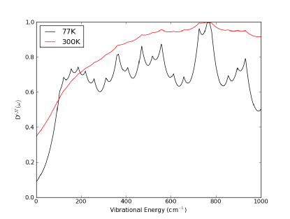
Figure 2: Effective vibrational density of states, calculated for PE545 assuming linewidth $\mathbb{L}(\Delta E)=e^{-\beta|\Delta E|}$.

Because of this, the assumption of a constant density of states may break down for pairs of chromophores which are close to degenerate, or at low temperatures. In these limits, $T_{i\rightarrow j}$ should be calculated using a finite summation in place of the integrals in Eq. 13.

The description of dynamics in PE545 was tested by calculating lineshapes for absorption, circular dichroism and fluorescence spectra, as well as the times necessary to transfer excitation between pairs of chromophores.

PE545 consists of six phycoerythrobilin (PEB) and two dihydrobiliverdin (DBV) chromophores, held in place by a dimer of two $\alpha\beta$ monomers. Each monomer contains three PEB chromophores on the $\beta$ subunit and one DBV chromophore on the $\alpha$ subunit. The DBV chromophores are redshifted with respect to the PEB chromophores, with absorption maxima at 569 nm, compared to 545 for the PEB chromophores van2006energy . Fig 1 shows the spatial arrangement of the chromophores in the complex. Excitons escape the comples by first making their way to the DBV bilins, then slowly settling onto the lowest energy DBV bilin before escaping the complex. Fluorescence experiments doust2006photophysics indicate that excitons primarily escape the complex via a single DBV bilin. Due to spectral overlap in the DBV and PEB bands, it may be difficult for spectroscopic experiments to distinguish precisely which chromophores are excited.

III.1 Static Lineshapes – Absorption, Fluorescence and Circular Dichroism

Spectra for absorption, circular dichroism and fluorescence can be calculated from time dependent expectation values of a density matrix which has been supplemented by addition of the ground state renger2002relation . Here the quantities of interest, $(a_{i}a^{*}_{j})(t)$ can be found by removing the thermodynamic weighting factors from the thermalized density matrix, in which the dynamics are calculated. The absorption spectrum is given by the Fourier transform of the dipole correlation function

$$d(t)=<\vec{\mu}(t)\vec{\mu}(0)>.$$ (19)

where the dipole operator $\vec{\mu}=\sum_{i}\vec{\mu_{i}}(\mathinner{|{i}\rangle}\mathinner{\langle{0}|}+\mathinner{|{0}\rangle}\mathinner{\langle{i}|})$. In terms of the density matrix, this is given by

$$d(t)=\text{Tr}(\vec{\mu}\vec{\rho}(t)),$$ (20)

where $\vec{\rho}(0)=\vec{\psi(0)}\bigotimes\vec{\psi^{*}}(0)$, $\vec{\psi(0)}=\mathinner{|{0}\rangle}+\epsilon\sum_{i}\vec{\mu_{i}}\mathinner{|{i}\rangle}$ and $\vec{\rho}(t)$ is found by propagating $\vec{\tilde{\rho}}$ according to Eq. 15. The parameter $\epsilon$ factors out of the Fourier transform and is discarded upon normalization of the spectrum. Dephasing between the ground and excited states is treated as an exponential decay term $\Gamma_{0i}=(400cm^{-1})$, taken from novoderezhkin2010excitation .

In the same way, the circular dichroism spectrum is found by taking the Fourier transform of

$$\vec{m}(t)=<\vec{m}(t)\vec{\mu}(0)>$$ (21)

where $\vec{m}=\vec{\mu}\times\vec{R}$ is the magnetic dipole operator. Figures 3 and 4 compare the calculated absorption and circular dichroism lineshapes to those measured in experiment in novoderezhkin2010excitation . Because the current theory does not account for reorganization energy of the chromophores following excitation, these spectra have been shifted in energy so that the peak of the calculated spectrum aligns with the peak of the experimental spectrum.

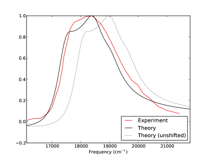
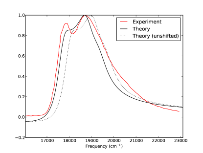
Figure 3: Normalized absorption spectra $\omega*d(\omega)$ for PE545, compared to experimental values taken from novoderezhkin2010excitation . a) 300K, b)77K.

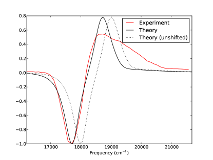
Figure 4: Normalized circular dichroism spectra $\omega*m(\omega)$ calculated at 300K compared to experimental values taken from novoderezhkin2010excitation .

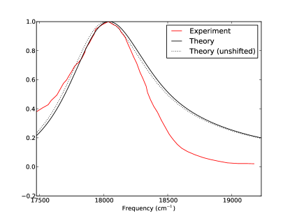
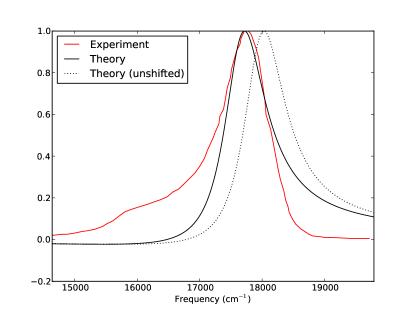
Figure 5: Normalized fluorescence spectra $\omega^{3}*d(\omega)$ for PE545, compared to experimental values taken from novoderezhkin2010excitation . a) 300K, b)77K.

In contrast to the absorption and circular dichroism spectra, the fluorescence spectrum reflects emission at large times, for a system which has settled into the lowest energy eigenstate. If this eigenstate is given by $\psi_{e}$ and $\psi(0)=\psi_{e}+\epsilon\mathinner{|{0}\rangle}$, the fluorescence spectrum is proportional to $w^{3}|\vec{f}(\omega)|^{2}$, where

$$\vec{f}(t)=<\vec{\mu}\rho(t)>$$ (22)

and $\rho(0)=\psi(0)\bigotimes\psi(0)$. Figure 5 compares the normalized fluorescence spectrum to that measured in experiment.

At 300K, the calculated lineshapes show good agreement. The width of the absorption and the negative lobe of the circular dichroism spectra agree closely with the experimental widths, although the positive lobe of the circular dichroism spectrum has a broader tail and less accentuated peak than the calculated lobe. The calculated fluorescence spectrum agrees with experiment in the peak region and on the blue side of the maximum, but falls off more quickly than experiment on the red side of the maximum.

Agreement with experiment is somewhat worse at 77K. The absorption spectrum gives the correct width in the peak region, but falls off more quickly than experiment on the red side of the maximum and less quickly than experiment on the blue side. The fluorescence spectrum shows good agreement with the experimental lineshape on the blue side of the maximum, but falls off much more quickly than the experiment on the red side. Both the absorption and fluorescence spectra miss a broad tail on the red side of the fluorescence. The circular dichroism spectrum at 77K was not available for comparison.

III.2 Exciton Transfer Times

While static lineshapes incorporate some dynamical information in the form of a Fourier transform of a time dependent correlation function, this information is obscured somewhat by the thermodynamic factors favoring population of low energy chromophores and by finite linewidths due to the decay of coherence. In doust2005mediation ,timescales for exciton transfer were measured more directly by finding Evolution Associated Difference Spectra (EADS) associated with particular transfer lifetimes following an excitation pulse of a particular frequency. Here interpretation is complicated by spectral overlap between chromophores, and by the difficulty in distinguishing between similar transfer lifetimes, so that only a few, picosecond scale lifetimes could be measured, and the chromophores being populated/depopulated could not be completely identified.

Within these limitations, the calculated rates for exciton transfer show good agreement with experiment. Table 6 shows the experimentally measured EADS transfer times, measured at 300K and 77K, for excitation wavelengths of 485 nm and 530 nm. Tables 8 and 7 show experimental decay times $\lambda_{+}^{-1}$, calculated using Eq. 17.

T (k)	$\lambda_{\text{excitation}}$ (nm)	T1 (fs)	T2 (fs)	T3 (ps)	T4 (ps)	T5 (ns)
298	485	25	250	1.84	23.5	1
298	530	25	250	1.84	16.4	$>1$
77	485	25	960	3.0	30	$>1$
77	530	25	960	3.0	17.7	$>1$

Figure 6: Experimentally measured transfer times, taken from doust2005mediation .

	$\beta_{50C}$	$\alpha_{19A}$	$\alpha_{19B}$	$\beta_{82C}$	$\beta_{158C}$	$\beta_{50D}$	$\beta_{82D}$	$\beta_{158D}$
$\beta_{50C}$					3.7
$\alpha_{19A}$			8.4	0.96
$\alpha_{19B}$		8.4		$0.06+0.09i$
$\beta_{82C}$		0.96	$0.06+0.09i$
$\beta_{158C}$	3.7
$\beta_{50D}$
$\beta_{82D}$								7.7
$\beta_{158D}$							7.7

Figure 7: Transfer / coherence decay times (ps) shorter than 100 ps for PE545 calculated at 77K.

	$\beta_{50C}$	$\alpha_{19A}$	$\alpha_{19B}$	$\beta_{82C}$	$\beta_{158C}$	$\beta_{50D}$	$\beta_{82D}$	$\beta_{158D}$
$\beta_{50C}$			2.93	2.11	1.21	4.81	12.9	14.9
$\alpha_{19A}$			20.4	2.64	7.37		19.3
$\alpha_{19B}$	2.93	20.4		0.158				27.2
$\beta_{82C}$	2.11	2.64	0.158
$\beta_{158C}$	1.21	7.37				53.5	28.7	25.3
$\beta_{50D}$	4.81				53.5		2.11	7.75
$\beta_{82D}$	12.9	19.3			28.7	2.11		8.67
$\beta_{158D}$	14.9		27.2		25.3	7.75	8.67

Figure 8: Transfer / coherence lifetimes (ps) shorter than 100 ps for PE545 calculated at 300K.

As with static spectra, agreement between theory and experiment is somewhat better at 300K than at 77K. At 300K, population of a DBV chromophore is found to occur in 150 fs, vs an experimentally measured 250 fs, while transfer of population between DBV chromophores is calculated to occur in 20.4 ps, compared to an experimental value of 23.4 ps or 16.4 ps, depending on the excitation frequency. Several pairs of chromophores are calculated to have transfer times in the range of 1-3 ps, comparable to the remaining experimental rate of 1.84 ps.

Agreement with experiment is considerably worse at 77K. Population of a DBV chromophore is now calculated to occur in 956 fs, compared to an experimental value of 960 fs, while a 3.7 ps time for transfer between $\beta_{50C}$ and $\beta_{158C}$ matches well with a 3 ps experimental transfer times. However, the 8.4 ps calculated for transfer between DBV chromophores and the 7.7 ps calculated between $\beta_{50D}$ and $\beta_{82D}$ do not correspond well with experimental times of 30 ps and 17.7 ps. Finally, the theoretical calculations include an underdamped transfer between $\alpha_{19B}$ and $\beta_{82C}$ which is not seen in the experiment, perhaps because the real part of the transfer time, at 60 fs, is shorter than the experimental resolution of 120 fs.

III.3 Density Matrix Propagation vs. Pairwise Decay Model

The agreement between the calculated pairwise decay times and transfer times measured in experiment raise the question of which information in $\tilde{\rho}$ is necessary to describe the dynamics of excitons in the complex. In principle, the entire density matrix is necessary to describe these dynamics, as excitons may follow any pathway through the complex, so that the amplitude to be on any particular chromophore is the sum of many interfering pathways. However, due to thermodynamic weighting of the effective coupling matrix, many of these pathways are strongly overdamped, with weak effective coupling and slow decay of any population imbalance. Because of this, the network of efficient transfer pathways is relatively sparse. This can be seen in Tables 8 and 7, or pictorially in Figure 9, where the opacity of the line connecting two chromophores reflects the rate of decay for population imbalances $(\tilde{\rho}_{ii}-\tilde{\rho}_{jj})$ (or antisymmetric coherence terms $(\tilde{\rho}_{ij}-\tilde{\rho}_{ji})$) between them. As a result of this sparsity, there are relatively few efficient pathways through the complex which may interfere with each other effectively. In Figure 9, two interfering pathways would form a closed curve of lines with nearly equal opacity.

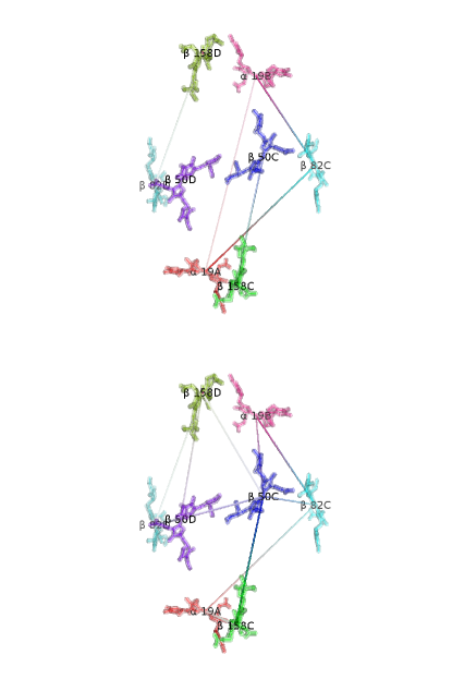
Figure 9: Rates of population transfer / coherence decay in PE545. Lines connecting chromophores have opacity proportional to $\lambda_{+}^{-1}$, with full opacity corresponding to $\lambda_{+}^{-1}=1$ ps. a) Rates calculated at 77K b) Rates calculated at 300K.

At 77K, $\alpha_{19A}$, $\beta_{82C}$ and $\alpha_{19B}$ form the only closed curve, while none are present at 300K (the 150 fs transfer time between $\alpha_{19B}$ and $\beta_{82C}$ is much faster than the  2 ps transfer times between $\alpha_{19B},\beta_{158C}$ and $\beta_{82C},\beta_{158C}$).

Due to the lack of interfering pathways, the flow of excitons through the PE545 antenna complex is well approximated by a minimal model, in which population imbalances in the thermalized density matrix decay exponentially as

$$\frac{d}{dt}(\tilde{\rho}_{ii}-\tilde{\rho}_{jj})=-\lambda_{+}(\tilde{\rho}_{ii}-\tilde{\rho}_{jj}),$$ (23)

with $\lambda_{+}$ given by Eq. 17.

The close agreement between the minimal model and the full density matrix propagation is shown in Figures 10, 11, 12, 13, 14, 15, 16, and 17, which compare the two models for initial conditions with the excitons localized on each individual chromophore. The largest departure between the two models is observed for $\alpha_{19A}$, $\beta_{82C}$ and $\alpha_{19B}$ initial conditions at 77K, which correspond to the closed curve of efficient transfer pathways previously identified.

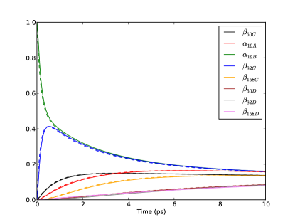
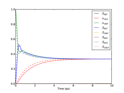
Figure 10: Exciton populations vs time calculated at a) 300K b) 77K for initial state $\alpha_{19B}$. Solid lines give populations calculated by Eq. 15, while dashed lines give populations calculated using the minimal exponential decay model.

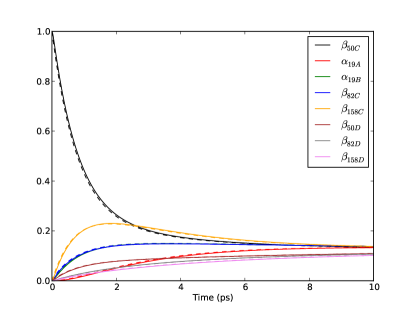
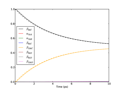
Figure 11: Exciton populations vs time calculated at a) 300K b) 77K for initial state $\beta_{50C}$. Solid lines give populations calculated by Eq. 15, while dashed lines give populations calculated using the minimal exponential decay model.

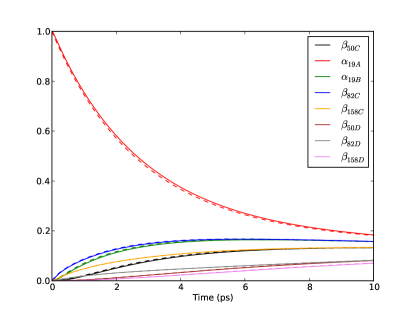
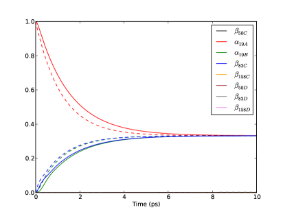
Figure 12: Exciton populations vs time calculated at a) 300K b) 77K for initial state $\alpha_{19A}$. Solid lines give populations calculated by Eq. 15, while dashed lines give populations calculated using the minimal exponential decay model.

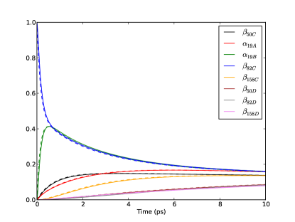
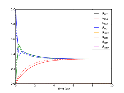
Figure 13: Exciton populations vs time calculated at a) 300K b) 77K for initial state $\beta_{82C}$. Solid lines give populations calculated by Eq. 15, while dashed lines give populations calculated using the minimal exponential decay model.

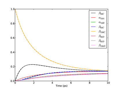
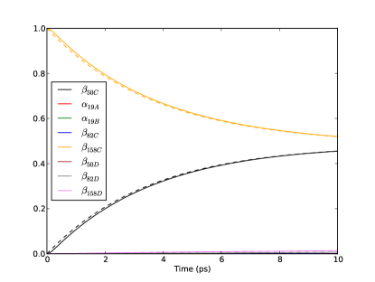
Figure 14: Exciton populations vs time calculated at a) 300K b) 77K for initial state $\beta_{158C}$. Solid lines give populations calculated by Eq. 15, while dashed lines give populations calculated using the minimal exponential decay model.

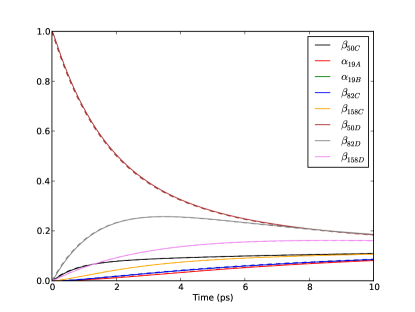
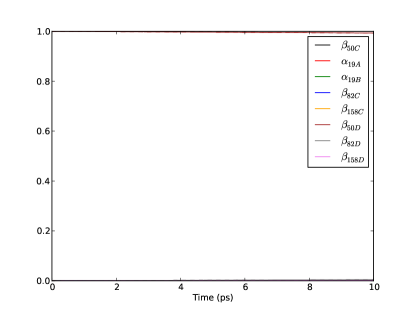
Figure 15: Exciton populations vs time calculated at a) 300K b) 77K for initial state $\beta_{50D}$. Solid lines give populations calculated by Eq. 15, while dashed lines give populations calculated using the minimal exponential decay model.

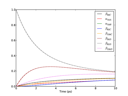
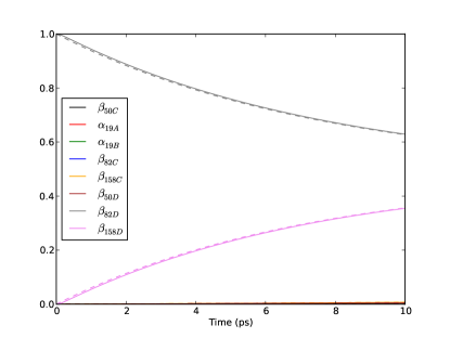
Figure 16: Exciton populations vs time calculated at a) 300K b) 77K for initial state $\beta_{82D}$. Solid lines give populations calculated by Eq. 15, while dashed lines give populations calculated using the minimal exponential decay model.

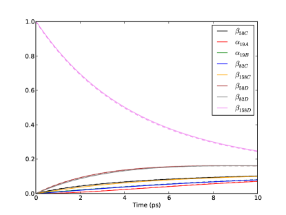
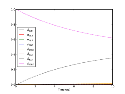
Figure 17: Exciton populations vs time calculated at a) 300K b) 77K for initial state $\beta_{158D}$. Solid lines give populations calculated by Eq. 15, while dashed lines give populations calculated using the minimal exponential decay model.

The close agreement between the two models explains why the experimental transfer rates show good agreement with the pairwise transfer rates, and indicates that the information contained in the long lived antisymmetric coherence terms, which are not included in the exponential decay model, does not play a vital role in the transfer of exciton population. Although the antisymmetric coherence terms show the same picosecond timescales for decay as the population imbalances, the lack of efficient, closed cycles in the PE545 complex leave little opportunity for interference. In addition, all initial conditions settle rapidly to the same equilibrium distribution at 300K, so that any ”quantum speedup” would offer only transient advantages. For these reasons, it appears that the importance of coherence terms in PE545 is dynamic rather than informational – coherence terms are important because they are required to give the correct transfer rates between chromophores, but the information contained in these terms does not appear to play an essential role in the transfer of the exciton population to the radiating DBV chromophore.

IV Conclusions

This paper has presented a new theory of coherent dynamics in photosynthetic complexes. Strong interaction with a reservoir causes rapid thermalization of vibrational states, allowing equations of motion for slowly varying electronic coefficients to be derived. By incorporating thermodynamic quantities into the definition of a thermalized density matrix and an effective coupling, these equations of motion are reduced to the Haken, Reineker, Strobl form. Unlike the original HRS model, the incorporation of thermodynamic information causes the system to settle to the correct thermodynamic equilibrium rather than to equal population of all states. The resulting theory gives good theoretical lineshapes for absorption, fluorescence and circular dichroism for PE545 at 300K and 77K, and yields exciton transfer times which agree with those found by EADS experiments. For both kinds of experiments, agreement is better at 300K than at 77K.

Long lived coherences between chromophores, such as those observed in lee2007coherence ; collini2010coherently ; gregory2007evidence ; savikhin1997oscillating , are simply explained in terms of an overdamped harmonic oscillator, in which the strength of the damping is proportional to the temperature and the effective coupling decreases exponentially with the excitation energy separation between two chromophores. Because of this, coherence terms may survive for arbitrarily long times, even in the high temperature limit for a system which interacts strongly with its environment.

Somewhat surprisingly, the long lifetime for survival of coherence terms appears to have a minimal effect on the transfer of exciton population in the PE545 antenna complex. This can be understood as resulting from the relatively sparse network of efficient transfer pathways in this complex, which has the effect of limiting interference between competing pathways. A minimal exponential decay model describes the flow of exciton population through this network accurately at 300K, when this network has no closed cycles, but departs from the full density matrix calculation at 77K, when such a cycle allows for interference between multiple pathways through the complex. It is possible that other photosynthetic molecules, with functions more sophisticated than the simple direction of exciton population to the lowest energy chromophore, may make more sophisticated use of this information.

The method of thermalized reduction of the density matrix introduced in this paper allows the derivation of quantum coherent equations of motion in a regime of high temperature and strong interaction with the surrounding environment which is often considered inimical to quantum mechanical behavior. Rather than being destroyed rapidly by interaction with the reservoir, coherence terms may persist or even be preserved by interaction with the reservoir. The conditions necessary for reduction – that the reduced degrees of freedom thermalize rapidly with respect to the evolution of the unreduced degrees of freedom – are satisfied in the limit of strong interaction with the reservoir, while the thermodynamic weighting of the effective coupling matrix may yield slow evolution of the unreduced degrees of freedom even when the bare coupling is relatively strong. The simplicity of the conditions necessary for the thermalized reduction procedure show that quantum mechanical behavior does not require low temperatures or elaborate isolation from the surroundings to be observed.

V Acknowledements

This work was supported in part by the SAW grant of the Liebniz society.

References

- (1) Lee, H., Cheng, Y. & Fleming, G. Coherence dynamics in photosynthesis: protein protection of excitonic coherence. Science 316, 1462 (2007).
- (2) Collini, E. et al. Coherently wired light-harvesting in photosynthetic marine algae at ambient temperature. Nature 463, 644–647 (2010).
- (3) Gregory, S., Tessa, R., Elizabeth, L., Tae-Kyu Ahn, T. et al. Evidence for wavelike energy transfer through quantum coherence in photosynthetic systems. Nature 446, 782–786 (2007).
- (4) Savikhin, S., Buck, D. & Struve, W. Oscillating anisotropies in a bacteriochlorophyll protein: Evidence for quantum beating between exciton levels. Chemical physics 223, 303–312 (1997).
- (5) van Grondelle, R. & Novoderezhkin, V. Quantum design for a light trap. Nature 463, 614–615 (2010).
- (6) Beljonne, D., Curutchet, C., Scholes, G. & Silbey, R. Beyond Forster resonance energy transfer in biological and nanoscale systems. The Journal of Physical Chemistry B 113, 6583–6599 (2009).
- (7) Ishizaki, A. & Fleming, G. On the adequacy of the Redfield equation and related approaches to the study of quantum dynamics in electronic energy transfer. The Journal of chemical physics 130, 234110 (2009).
- (8) May, V. & Kühn, O. Charge and energy transfer dynamics in molecular systems (Wiley Online Library, 2004).
- (9) Haken, H. & Strobl, G. An exactly solvable model for coherent and incoherent exciton motion. Zeitschrift für Physik A Hadrons and Nuclei 262, 135–148 (1973).
- (10) Čápek, V. Generalized haken-strobl-reineker model of excitation transfer. Zeitschrift für Physik B Condensed Matter 60, 101–105 (1985).
- (11) Diósi, L. & Strunz, W. The non-markovian stochastic schrödinger equation for open systems. Physics Letters A 235, 569–573 (1997).
- (12) Strunz, W. Linear quantum state diffusion for non-markovian open quantum systems. Physics Letters A 224, 25–30 (1996).
- (13) Mohseni, M., Rebentrost, P., Lloyd, S. & Aspuru-Guzik, A. Environment-assisted quantum walks in photosynthetic energy transfer. The Journal of chemical physics 129, 174106 (2008).
- (14) Rebentrost, P., Mohseni, M., Kassal, I., Lloyd, S. & Aspuru-Guzik, A. Environment-assisted quantum transport. New Journal of Physics 11, 033003 (2009).
- (15) Caruso, F., Chin, A., Datta, A., Huelga, S. & Plenio, M. Highly efficient energy excitation transfer in light-harvesting complexes: The fundamental role of noise-assisted transport. Journal of Chemical Physics 131, 105106 (2010).
- (16) Sarovar, M., Ishizaki, A., Fleming, G. & Whaley, K. Quantum entanglement in photosynthetic light-harvesting complexes. Nature Physics 6, 462–467 (2010).
- (17) Hoyer, S., Sarovar, M. & Whaley, K. Limits of quantum speedup in photosynthetic light harvesting. New Journal of Physics 12, 065041 (2010).
- (18) Unruh, W. Maintaining coherence in quantum computers. Physical Review A 51, 992 (1995).
- (19) Scholes, G. Long-range resonance energy transfer in molecular systems. Annual review of physical chemistry 54, 57–87 (2003).
- (20) Breuer, H. & Petruccione, F. The theory of open quantum systems (Oxford University Press, USA, 2002).
- (21) Novoderezhkin, V., Doust, A., Curutchet, C., Scholes, G. & van Grondelle, R. Excitation dynamics in phycoerythrin 545: Modeling of steady-state spectra and transient absorption with modified redfield theory. Biophysical journal 99, 344–352 (2010).
- (22) van Grondelle, R. & Novoderezhkin, V. Energy transfer in photosynthesis: experimental insights and quantitative models. Physical Chemistry Chemical Physics 8, 793–807 (2006).
- (23) Doust, A., Wilk, K., Curmi, P. & Scholes, G. The photophysics of cryptophyte light-harvesting. Journal of Photochemistry and Photobiology A: Chemistry 184, 1–17 (2006).
- (24) Renger, T. & Marcus, R. On the relation of protein dynamics and exciton relaxation in pigment–protein complexes: An estimation of the spectral density and a theory for the calculation of optical spectra. The Journal of chemical physics 116, 9997 (2002).
- (25) Doust, A. et al. Mediation of ultrafast light-harvesting by a central dimer in phycoerythrin 545 studied by transient absorption and global analysis. The Journal of Physical Chemistry B 109, 14219–14226 (2005).