Description of fully differential Drell-Yan pair production

Abstract

We investigate Drell-Yan pair production in a QCD inspired model, which takes into account all relevant hard processes up to $O(\alpha_{s})$. To address the known shortfalls of such a fixed order calculation we introduce phenomenological parton distributions for initial transverse momentum and quark mass, and devise a subtraction scheme to avoid double-counting when utilizing the standard longitudinal parton distribution functions. We show that we can reproduce Drell-Yan transverse momentum and invariant mass spectra from different proton-proton, proton-nucleus and antiproton-nucleus experiments and at different energies without the need for a $K$ factor. Fixing our parameters at these spectra, we make predictions for Drell-Yan transverse momentum spectra at low hadronic energies, which will be measured for example at $\overline{\text{P}}$ANDA in antiproton-proton collisions.

I Introduction

The Drell-Yan (DY) process Drell and Yan (1970) has been studied for the last 40 years and provides an important tool to access the distribution of partons inside the nucleon. While the primary tool for exploration of the nucleon structure is deep inelastic scattering Bjorken and Paschos (1969), DY data give complementary insights, since, for example, it directly probes sea-quark distributions Alekhin et al. (2006). A lot of experimental effort is being devoted to measurements of the DY process: in antiproton-proton ($\overline{\text{p}}$p) collisions at $\overline{\textrm{P}}$ANDA (FAIR) The PANDA collaboration et al. (2009) and PAX Barone et al. (2005), in proton-proton (pp) collisions at RHIC Bunce et al. (2000, 2008), J-PARC Peng et al. (2006); Goto et al. (2007); Kumano (2008), IHEP Abramov et al. (2005) and JINR Sissakian et al. (2009) and in pion-nucleon collisions at COMPASS Bradamante (1997); Baum et al. (1996). An overview of the experimental situation can be found in Reimer (2007).

Studies of this process Halzen and Scott (1978); Altarelli et al. (1978); Arnold et al. (2009) are generally inspired by perturbative QCD (pQCD). The most simple scheme is the parton model description, which is a leading order (LO) approach ($O(\alpha_{s}^{0}$)). However, it does not fully describe the interesting observables. While the shape of the invariant mass ($M$) spectra of the DY pair can be reproduced, the absolute height can only be accounted for by including an additional $K$ factor. Furthermore transverse momentum ($p_{T}$) spectra are not accessible at all Gavin et al. (1995). The usual approach to handle the latter problem is to fold in a phenomenological Gaussian distribution for the parton transverse momentum D’Alesio and Murgia (2004), the width of which has to be fitted to data. But since these distributions are normalized, the absolute size of the cross sections is still underestimated D’Alesio and Murgia (2004). The next logical step is to turn to next-to-leading order (NLO, $O(\alpha_{s})$) in the contributing hard subprocesses, but this brings about additional problems: the calculated $p_{T}$ spectra are divergent for $p_{T}\rightarrow 0$. In fact, they are divergent in any fixed order of the strong coupling $\alpha_{s}$, due to large logarithmic corrections $\ln\left(M/p_{T}\right)$ Gavin et al. (1995). It is possible to remove these divergences by an all-order resummation. However, since $p_{T}$ is no longer a hard scale at $p_{T}\rightarrow 0$, additional non-perturbative (i.e., experimental) input is needed in these (and all other pQCD) approaches to describe the region of very small $p_{T}$ Collins et al. (1985); Davies et al. (1985); Fai et al. (2003). Note that the parton model (i.e., LO) description is still a very useful starting point, for example for studying spin asymmetries in DY, since there NLO corrections appear to be rather small Shimizu et al. (2005); Barone et al. (2006); Martin et al. (1998). $\overline{\textrm{P}}$ANDA, however, will allow measurements at hadron c.m. energies of a few GeV, where non-perturbative effects are expected to become more important. This highlights the need to model these effects in a phenomenological picture.

In Eichstaedt et al. (2010) we revisited a model, which incorporates phenomenological transverse momentum distributions for quarks and which takes into account the full kinematics in the hard LO subprocess, i.e., the usual collinear approximation is overcome. It was found that results differed only slightly from standard parton model calculations, which underestimate the data. In the present paper we improve on our previous work in several ways: First, we include quark mass distributions in the LO process. We will show that we still underestimate the data. This finding triggered a complete calculation of all hard subprocesses to $O(\alpha_{s})$ including the full kinematics, which will also be presented in the current work. As mentioned above, such a calculation would suffer from divergent $p_{T}$ spectra if the quarks were massless. However, we will show that the phenomenological quark mass distributions we introduced before now effectively smear out the divergent behavior. Such mass distributions or spectral functions are a well known concept in nuclear physics, where they are applied to the strongly coupled system of nucleons in nuclei, see for example Day et al. (1990). Thus it is worthwhile to test the same concept in the nucleon, which is a strongly coupled system of quarks and gluons. For ($p_{T}$ integrated) $M$ spectra the divergent $O(\alpha_{s})$ contributions are commonly absorbed into the parton distribution functions. Therefore, we introduce a subtraction scheme to prevent double counting of those processes which we consider explicitly.

This paper is structured as follows: We introduce our notation and conventions in Sec. I.1 and we give an introduction to the general kinematics of DY pair production in Sec. I.2. In Sec. II we address DY at LO, in particular we describe the standard parton model and our extensions of it, namely including intrinsic parton transverse momentum and quark mass distributions. We show the results of our extended LO model in Sec. II.5. Sec. III presents our NLO calculation. The vertex correction is treated in detail in III.1 and the calculation of gluon bremsstrahlung and gluon Compton scattering is presented in Secs. III.2 and III.3. In Sec. III.4 the influence of quark mass distributions is discussed. Furthermore, we discuss the treatment of collinear singularities and describe our subtraction scheme for the $O(\alpha_{s})$ contributions in detail in Sec. III.5, before we shortly comment on the use of initial transverse momentum distributions. We show the results of our full model in Sec. IV and compare with data from different experiments in pp, p-nucleus and $\overline{\text{p}}$-nucleus reactions. In addition we present our predictions for DY pair production at $\overline{\textrm{P}}$ANDA energies. Finally we present our conclusions in Sec. V. The Appendix collects several topics, that are only briefly touched in the main text: since we assign different masses to the annihilating quarks and antiquarks, we explicitly prove gauge invariance in App. A. Then we investigate the influence of different quark masses on the form factors $F_{1}$ and $F_{2}$ in App. B, and finally we present the details of the phase space evaluation in App. C.

I.1 Notation

In the following we present the conventions and notations used throughout this paper: It will turn out to be useful to write four-momenta using light-cone coordinates. We employ the following convention for general four-vectors $a$ and $b$:

$$a^{+} =a_{0}+a_{z}\ ,$$ (1)

$$a^{-} =a_{0}-a_{z}\ ,$$ (2)

$$\vec{a}_{\perp} =\left(a_{x},a_{y}\right)\ ,$$ (3)

$$\Rightarrow a^{2} =a^{+}a^{-}-({\vec{a}}_{\perp})^{2}\ ,$$ (4)

$$\Rightarrow a\cdot b =\frac{1}{2}\left(a^{+}b^{-}+a^{-}b^{+}-2\,\vec{a}_{\perp}\cdot\vec{b}_{\perp}\right)\ .$$ (5)

Leptons are treated as massless. We define the target nucleon to carry the four-momentum $P_{1}$ and the beam nucleon to carry the four-momentum $P_{2}$ (see Fig. 1). In the hadron center-of-mass (c.m.) frame we choose the $z$-axis as the beam line, and the beam (target) nucleon moves in the positive (negative) direction. Therefore, the nucleon four-momenta read

$$P_{1} =\left(\frac{\sqrt{S}}{2},0,0,-\sqrt{\frac{S}{4}-m_{N}^{2}}\right)\ ,$$ (6)

$$P_{2} =\left(\frac{\sqrt{S}}{2},0,0,+\sqrt{\frac{S}{4}-m_{N}^{2}}\right)\ ,$$ (7)

which implies

$$P_{1}^{-}=P_{2}^{+}=\frac{\sqrt{S}}{2}+\sqrt{\frac{S}{4}-m_{N}^{2}}\xrightarrow{m_{N}\rightarrow 0}\sqrt{S}$$ (8)

for the large momentum components of the nucleons. Note that in Eichstaedt et al. (2010) we presented a calculation with vanishing nucleon mass $m_{N}$. However, we want to study our model also at comparatively low c.m. energies (e.g. $\sqrt{S}\sim 5.5$ GeV at $\overline{\textrm{P}}$ANDA). Therefore, in the present work we include the nucleon mass since its influence should become significant at these energies. We denote the four-momentum of the parton in nucleon 1 (2) as $p_{1}$ ($p_{2}$). The on-shell condition in light-cone coordinates then reads:

$$m_{i}^{2}=p_{i}^{2}=p_{i}^{+}p_{i}^{-}-({\vec{p}}_{i_{\perp}})^{2}\ .$$ (9)

For the virtual photon in Fig. 1 the maximal $q_{z}$ is derived by requiring the invariant mass of the undetected remnants to vanish and the photon to move collinearly to the nucleons:

$$\left(P_{1}+P_{2}-q\right)^{2} =X^{2}\overset{!}{=}0$$ (10)

$$\Rightarrow S+q^{2}-2\sqrt{S}\sqrt{q^{2}+(q_{z})_{\textrm{max}}^{2}} =0$$ (11)

$$\Rightarrow\frac{S-q^{2}}{2\sqrt{S}} =(q_{z})_{\textrm{max}}\ .$$ (12)

In the literature and in the data presented by many experimental groups the Feynman variable Nakamura et al. (2010) is defined as:

$$x_{F} =\frac{2q_{z}}{\sqrt{S}}\simeq\frac{q_{z}}{(q_{z})_{\textrm{max}}}$$

$$\Rightarrow(q_{z})_{\textrm{max}} \simeq\frac{\sqrt{S}}{2}\ .$$ (13)

Note that this approximation for $x_{F}$ is obviously only valid for $q^{2}\ll S$. Since we perform studies in the small-$S$ region, our definition of the Feynman variable $x_{F}^{\prime}$ is :

$$x_{F}^{\prime}=\frac{q_{z}}{(q_{z})_{\textrm{max}}}=q_{z}\cdot\frac{2\sqrt{S}}{S-q^{2}}\ ,$$ (14)

without any approximations. Depending on the experiment which we study we will use $x_{F}$ or $x_{F}^{\prime}$ according to Eq. (13) and Eq. (14) .

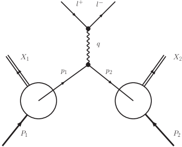
Figure 1: DY production in a nucleon-nucleon collision; $X_{1}$ and $X_{2}$ denote the nucleon remnants. See main text for details.

I.2 General kinematics

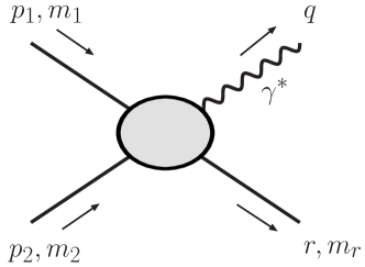
Figure 2: General kinematics of hard subprocesses of DY production.

In this section we shortly present the kinematic scheme, in which our calculations are performed. Note that we show the most general form for DY pair production at NLO, of which the LO process is a special case. Fig. 2 is a reference for our notation.

For the initial particles we choose four-momenta $p_{1}$ and $p_{2}$ and masses $m_{1}$ and $m_{2}$. For the final state we always choose $q$ as the four-momentum of the virtual photon, i.e., the DY pair, and $M=\sqrt{q^{2}}$ as its mass. The four-momentum of the remaining final state particle we define as $r$ and its mass as $m_{r}$ (both $0$ at LO). The differential partonic cross section then takes the following general form:

$$\textrm{d}\hat{\sigma}=F(p_{1},p_{2},q,r)\cdot\delta^{(4)}(p_{1}+p_{2}-q-r)\,\textrm{d}M^{2}\,\frac{\textrm{d}^{3}q}{E_{q}}\,\frac{\textrm{d}^{3}r}{2E_{r}}\ ,$$ (15)

where $F$ contains squared matrix elements, the flux factor and constants, and $E_{q}$ ($E_{r}$) are the energies of the particles with momenta $q$ ($r$). Note that in the LO case there is only the virtual photon in the final state and thus

$$F(p_{1},p_{2},q,r)=\tilde{F}(p_{1},p_{2},q)\cdot\delta^{(4)}(r)\,2E_{r}\textrm{d}E_{r}\ .$$ (16)

The Mandelstam variables read

$$s =(p_{1}+p_{2})^{2}\ ,$$ (17)

$$t =(p_{2}-q)^{2}\ ,$$ (18)

$$u =(p_{1}-q)^{2}\ .$$ (19)

In DY measurements the common observables are the invariant mass $M$, the absolute transverse momentum $p_{T}$ and the longitudinal momentum $q_{z}$ of the lepton pair. Thus we can integrate Eq. (15) over the phase space of $r$ as well as the azimuthal angle $\phi_{q}$ of $q$. Then we obtain

$$\frac{\textrm{d}\hat{\sigma}}{\textrm{d}M^{2}\textrm{d}t}=\frac{\pi}{2\sqrt{s}p_{\text{cm}}}\cdot F(s,t,M^{2},m_{1}^{2},m_{2}^{2},m_{r}^{2})\cdot\Theta(\sqrt{s}-E_{q})\ ,$$ (20)

with the center-of-mass momentum of the incoming states Nakamura et al. (2010)

$$p_{\text{cm}}=\frac{\sqrt{(s-(m_{1}+m_{2})^{2})(s-(m_{1}-m_{2})^{2})}}{2\sqrt{s}}\ .$$ (21)

Now comparing Eqs. (15) and (20) one finds (cf. Halzen and Scott (1978))

$$\frac{E_{q}\textrm{d}\hat{\sigma}}{\textrm{d}M^{2}\textrm{d}^{3}q}=\frac{2\sqrt{s}p_{\text{cm}}}{\pi}\cdot\frac{\textrm{d}\hat{\sigma}}{\textrm{d}M^{2}\textrm{d}t}\cdot\delta\left((p_{1}+p_{2}-q)^{2}-m_{r}^{2}\right)$$ (22)

and finally

$$\frac{\textrm{d}\hat{\sigma}}{\textrm{d}M^{2}\textrm{d}p_{T}^{2}\textrm{d}x_{F}}= \frac{2\sqrt{s}p_{\text{cm}}(q_{z})_{\textrm{max}}}{E_{q}}\cdot\frac{\textrm{d}\hat{\sigma}}{\textrm{d}M^{2}\textrm{d}t}$$

$$\times\delta\left((p_{1}+p_{2}-q)^{2}-m_{r}^{2}\right)\ .$$ (23)

Thus, for all the relevant subprocesses we actually only have to calculate $\frac{\textrm{d}\hat{\sigma}}{\textrm{d}M^{2}\textrm{d}t}$ and we will use the relation (23) especially for the NLO calculation with two particles (virtual photon + quark/gluon) in the final state.

II Leading order Drell-Yan

In this section we will present an approach to DY pair production in LO in the hard subprocess, i.e., $O(\alpha_{s}^{0})$. We will start with the standard parton model approach and then remedy its shortcomings by introducing distributions for transverse momentum and mass of the annihilating quarks. Finally we will present the results of this LO approach.

II.1 Standard parton model

The LO DY differential cross section in the standard parton model reads Drell and Yan (1970)

$$\textrm{d}\sigma_{\text{LO}}=$$

$$\int_{0}^{1}\textrm{d}x_{1}\int_{0}^{1}\textrm{d}x_{2}\sum_{i}q_{i}^{2}\,f_{i}(x_{1},q^{2})\,f_{\,\bar{i}}(x_{2},q^{2})\,\textrm{d}\hat{\sigma}(x_{1},x_{2},q^{2})\ .$$ (24)

The sum runs over all quark flavors and antiflavors, $q_{i}$ denotes the electric charge of quark flavor $i$ and the functions $f_{i}$ are parton distribution functions (PDFs).

As usual, $x_{1}$ and $x_{2}$ are the momentum fractions carried by the annihilating partons inside the colliding nucleons,

$$p_{1} =x_{1}P_{1}\ ,$$ (25)

$$p_{2} =x_{2}P_{2}\ .$$ (26)

Note that this implies

$$p_{1}^{-} =x_{1}P_{1}^{-}\ ,$$ (27)

$$p_{2}^{+} =x_{2}P_{2}^{+}$$ (28)

for the large parton momentum components. The small components are

$$p_{1}^{+}=\frac{m_{1}^{2}}{p_{1}^{-}}\ ,$$ (29)

$$p_{2}^{-}=\frac{m_{2}^{2}}{p_{2}^{+}}\ ,$$ (30)

and they are generally neglected in the standard parton model, since the partons are assumed to be massless. Consistency with the relations (25, 26) is then achieved by assuming also the nucleon mass to be negligible.

$\textrm{d}\hat{\sigma}$ is the differential cross section of the partonic subprocess,

$$\textrm{d}\hat{\sigma}_{\text{LO}}=\frac{4\pi\alpha^{2}}{9q^{2}}\,\delta(M^{2}-q^{2})\,\delta^{(4)}(p_{1}+p_{2}-q)\,\textrm{d}^{4}q\,\textrm{d}M^{2}\ ,$$ (31)

and so we find

$$\frac{\textrm{d}\hat{\sigma}_{\text{LO}}}{\textrm{d}M^{2}\textrm{d}t}=\frac{4\pi\alpha^{2}}{9M^{2}}\,\delta(M^{2}-(p_{1}+p_{2})^{2})\,\delta(t)\ .$$ (32)

Here $q$ is the four-momentum of the virtual photon, $p_{1},p_{2}$ are the four-momenta of the partons (cf. Fig. 1) and $\alpha\approx 1/137$ is the fine-structure constant.

The factorization into hard (subprocess) and soft (PDFs) physics is proven in the collinear case at least for leading twist (expansion in $1/M$) in Collins et al. (1988).

Note that it becomes immediately clear from Eqs. (25) and (26) that the incoming partons move collinearly with the nucleons. According to four-momentum conservation in Eq. (31) no transverse momentum can therefore be generated for the virtual photon (and thus for the DY pair) in the LO process.

The maximal information about the DY pair that can be gained from Eq. (24) is double differential,

$$\frac{\textrm{d}\sigma_{\text{LO}}}{\textrm{d}M^{2}\ \textrm{d}x_{F}}=\sum_{i}q_{i}^{2}f_{i}(x_{1},M^{2})\,f_{\,\bar{i}}(x_{2},M^{2})\,\frac{4\pi\alpha^{2}}{9M^{2}}\,\frac{(q_{z})_{\textrm{max}}}{(P_{1}^{-})^{2}E_{\textrm{coll}}}\ ,$$ (33)

with

$$x_{1} =\frac{-(q_{z})_{\textrm{max}}\,x_{F}+E_{\textrm{coll}}}{P_{1}^{-}}\ ,$$ (34)

$$x_{2} =\frac{(q_{z})_{\textrm{max}}\,x_{F}+E_{\textrm{coll}}}{P_{1}^{-}}$$ (35)

and the energy of the collinear DY pair,

$$E_{\textrm{coll}}=\sqrt{M^{2}+\left((q_{z})_{\textrm{max}}\,x_{F}\right)^{2}}\ .$$ (36)

In this section we have presented the standard parton model solution for the LO DY cross section. The only quantities in this approach not determined by pQCD are the PDFs. These have to be obtained by fitting parametrizations to experimental data, mainly on deep inelastic scattering (DIS), but also on measurements of DY production itself Stirling (2008).

II.2 Intrinsic transverse momentum

As already mentioned above, no DY pair transverse momentum ($p_{T}$) is generated in the simple parton model approach. Nevertheless, measurements indicate a Gaussian form of the $p_{T}$ spectra at not too large $p_{T}$. This has been studied in approaches including initial quark transverse momentum distributions, e.g. D’Alesio and Murgia (2004); Anselmino et al. (2006). In Eichstaedt et al. (2010) we also presented an approach incorporating primordial quark transverse momentum to address this issue. However, we found that additional unphysical solutions for the momentum fractions $x_{i}$ appear, which have to be removed properly. These unphysical solutions are an artifact of rewriting the momentum variables using light-cone coordinates and they reveal themselves as one of two possible solutions of a quadratic equation. The correct solutions can always be identified by putting all transverse momenta to zero and then by checking whether the well known parton model solutions for the $x_{i}$ as given in Eqs. (34,35) are recovered. In Eichstaedt et al. (2010) we found that in the transverse momentum dependent approach the LO DY differential cross section reads

$$\textrm{d}\sigma_{\text{LO}}=\fint_{0}^{1}\textrm{d}x_{1}\fint_{0}^{1}\textrm{d}x_{2}\int\textrm{d}{\vec{p}}_{1_{\perp}}\int\textrm{d}{\vec{p}}_{2_{\perp}}$$

$$\times\sum_{i}q_{i}^{2}{\tilde{f}}_{i}(x_{1},{\vec{p}}_{1_{\perp}},q^{2}){\tilde{f}}_{\,\bar{i}}(x_{2},{\vec{p}}_{2_{\perp}},q^{2})\textrm{d}\hat{\sigma}(x_{1},{\vec{p}}_{1_{\perp}},x_{2},{\vec{p}}_{2_{\perp}},q^{2})\ .$$ (37)

The functions ${\tilde{f}}_{i}(x,{\vec{p}}_{\perp},q^{2})$ are now extensions of the standard longitudinal PDFs, since they also describe the distribution of quark transverse momentum. We will show our ansatz for these functions in Sec. II.4. Note that we take into account the full kinematics in the partonic cross section, i.e. $\textrm{d}\hat{\sigma}_{\text{LO}}=\textrm{d}\hat{\sigma}_{\text{LO}}(x_{1},{\vec{p}}_{1_{\perp}},x_{2},{\vec{p}}_{2_{\perp}},q^{2})$, however, the quark masses are neglected as in the previous section. In this approach the transverse momentum ($p_{T}=|{\vec{q}}_{\perp}|$) of the DY pair is accessible, since the annihilating quark and antiquark can have finite initial transverse momenta.

The symbol $\fint$ represents the requirement that the unphysical solutions for the $x_{i}$ have to be removed, as mentioned above. This is discussed in detail in Eichstaedt et al. (2010). Note that in the current paper we take into account a finite nucleon mass. Thus the following formulas for the momentum fractions $x_{i}$ are recovered from the corresponding formulas in Eichstaedt et al. (2010) by simply replacing $\sqrt{S}$ by $P_{1}^{-}$, cf. Eq. (8). Then we find for the triple-differential hadronic cross section:

$$\frac{\textrm{d}\sigma_{\text{LO}}}{\textrm{d}M^{2}\ \textrm{d}x_{F}\textrm{d}p_{T}^{2}}=\int_{0}^{2\pi}\textrm{d}\phi_{\perp}\int_{0}^{({\vec{k}}_{\perp})^{2}_{\textrm{max}}}\frac{1}{2}\textrm{d}{\vec{k}}_{\perp}^{\,2}\frac{\pi\ (q_{z})_{\textrm{max}}}{E}$$

$$\times \left|(P_{1}^{-})^{2}-\frac{(\hat{\vec{p}}_{1_{\perp}})^{2}(\hat{\vec{p}}_{2_{\perp}})^{2}}{(x_{1})_{-}^{2}(x_{2})_{+}^{2}(P_{1}^{-})^{2}}\right|^{-1}F_{\text{LO}}((x_{1})_{-},\hat{\vec{p}}_{1_{\perp}},(x_{2})_{+},\hat{\vec{p}}_{2_{\perp}},M^{2})$$ (38)

with

$$F_{\text{LO}}((x_{1})_{-},\hat{\vec{p}}_{1_{\perp}},(x_{2})_{+},\hat{\vec{p}}_{2_{\perp}},M^{2})=$$

$$\sum_{i}q_{i}^{2}\,{\tilde{f}}_{i}\left((x_{1})_{-},\hat{\vec{p}}_{1_{\perp}},M^{2}\right)\,{\tilde{f}}_{\,\bar{i}}\left((x_{2})_{+},\hat{\vec{p}}_{2_{\perp}},M^{2}\right)\,\frac{4\pi\alpha^{2}}{9M^{2}}\ ,$$ (39)

$$(x_{1})_{-}=$$

$$\frac{1}{P^{-}_{1}}\left(\frac{q^{-}}{2}-\frac{\vec{k}_{\perp}\cdot\vec{q}_{\perp}}{q^{+}}+\sqrt{\left(\frac{\vec{k}_{\perp}\cdot\vec{q}_{\perp}}{q^{+}}\right)^{2}+\frac{q^{-}}{q^{+}}\left(\frac{1}{4}M^{2}-\vec{k}_{\perp}^{\,2}\right)}\right)\ ,$$ (40)

$$(x_{2})_{+}=$$

$$\frac{1}{P_{1}^{-}}\left(\frac{q^{+}}{2}+\frac{\vec{k}_{\perp}\cdot\vec{q}_{\perp}}{q^{-}}+\sqrt{\left(\frac{\vec{k}_{\perp}\cdot\vec{q}_{\perp}}{q^{-}}\right)^{2}+\frac{q^{+}}{q^{-}}\left(\frac{1}{4}M^{2}-\vec{k}_{\perp}^{\,2}\right)}\right)\$$ (41)

and

$$\hat{\vec{p}}_{1_{\perp}} =\frac{1}{2}{\vec{q}}_{\perp}-{\vec{k}}_{\perp}\ ,$$ (42)

$$\hat{\vec{p}}_{2_{\perp}} =\frac{1}{2}{\vec{q}}_{\perp}+{\vec{k}}_{\perp}\ ,$$ (43)

$$E =\sqrt{M^{2}+p_{T}^{2}+x_{F}^{2}(q_{z})_{\textrm{max}}^{2}}$$ (44)

$$q^{+} =E+x_{F}(q_{z})_{\textrm{max}}\ ,$$ (45)

$$q^{-} =E-x_{F}(q_{z})_{\textrm{max}}\ ,$$ (46)

$$\left|{\vec{q}}_{\perp}\right| =p_{T}\ ,$$ (47)

$$\vec{k}_{\perp}\cdot\vec{q}_{\perp} =|\vec{k}_{\perp}|p_{T}\cos(\phi_{\perp})\ ,$$ (48)

$$({\vec{k}}_{\perp}^{\,2})_{\textrm{max}} =\frac{(M^{2}+p_{T}^{2})\frac{M^{2}}{4}}{M^{2}+p_{T}^{2}(1-\cos^{2}(\phi_{\perp}))}\ .$$ (49)

In Sec. II.5 we will show and compare the results of this approach to the standard parton model and the approach with mass distributions as described in Sec. II.3.

II.3 Quark masses

In Sec. II.2 we have extended the standard collinear PDFs towards quark distributions which also include quark transverse momentum. However, we have kept the masses of the quarks fixed at zero. Since in light cone coordinates the onshell condition reads $m^{2}=p^{2}=p^{+}p^{-}-({\vec{p}}_{\perp})^{2}$, this is equivalent to varying only two of the three, in principal independent quark momentum components $p^{+}$, $p^{-}$ and $p_{\perp}$. A fully unintegrated parton distribution should depend on all three of these components. Therefore, we once more extend the parton distributions of Sec. II.2 by

$${\tilde{f}}_{i}(x,{\vec{p}}_{\perp},q^{2})\rightarrow{\hat{f}}_{i}(x,{\vec{p}}_{\perp},m^{2},q^{2})\ .$$ (50)

We will present our ansatz for $\hat{f}$ in Sec. II.4. The differential hadronic cross section now becomes

$$\textrm{d}\sigma_{\text{LO}}= \fint_{0}^{1}\textrm{d}x_{1}\fint_{0}^{1}\textrm{d}x_{2}\int\textrm{d}{\vec{p}}_{1_{\perp}}\int\textrm{d}{\vec{p}}_{2_{\perp}}\int\textrm{d}{m_{1}^{2}}\int\textrm{d}{m_{2}^{2}}$$

$$\times\sum_{i}q_{i}^{2}{\hat{f}}_{i}(x_{1},{\vec{p}}_{1_{\perp}},m_{1}^{2},q^{2}){\hat{f}}_{\,\bar{i}}(x_{2},{\vec{p}}_{2_{\perp}},m_{2}^{2},q^{2})$$

$$\times\textrm{d}\hat{\sigma}(x_{1},{\vec{p}}_{1_{\perp}},x_{2},{\vec{p}}_{2_{\perp}},m_{1}^{2},m_{2}^{2},q^{2})\ .$$ (51)

The partonic cross section is now given by

$$\textrm{d}\hat{\sigma}_{\text{LO}}= \frac{4\pi\alpha^{2}}{9q^{4}}\frac{2q^{4}-q^{2}(m_{1}^{2}-6m_{1}m_{2}+m_{2}^{2})-(m_{1}^{2}-m_{2}^{2})^{2}}{2\sqrt{(q^{2}-m_{1}^{2}-m_{2}^{2})^{2}-m_{1}^{2}m_{2}^{2}}}$$

$$\times \,\delta(M^{2}-q^{2})\,\delta^{(4)}(p_{1}+p_{2}-q)\,\textrm{d}^{4}q\,\textrm{d}M^{2}\ .$$ (52)

Note that by assigning different masses $m_{1}$ and $m_{2}$ to the quarks, gauge invariance is not preserved at the quark-photon vertex. However, the unphysical polarization states of the virtual photon produced in this manner are projected out at the lepton-photon vertex and thus the entire amplitude is indeed gauge invariant. See Appendix A for details.

Now we have to perform the same procedure as described in Eichstaedt et al. (2010) to remove the unphysical solutions for the longitudinal momentum fractions $x_{i}$. In complete analogy we find (the details of this calculation can be found in Appendix C.2)

$$\frac{\textrm{d}\sigma_{\text{LO}}}{\textrm{d}M^{2}\ \textrm{d}x_{F}\textrm{d}p_{T}^{2}}= \int_{0}^{2\pi}\textrm{d}\phi_{\perp}\int_{0}^{({\vec{k}}_{\perp})^{2}_{\textrm{max}}}\frac{1}{2}\textrm{d}({\vec{k}}_{\perp})^{2}\int_{0}^{(m_{1})^{2}_{\textrm{max}}}\textrm{d}m_{1}^{2}\int_{0}^{(m_{2})^{2}_{\textrm{max}}}\textrm{d}m_{2}^{2}\ \frac{\pi\ (q_{z})_{\textrm{max}}}{E}$$

$$\times\left|\left(P_{1}^{-}\right)^{2}-\frac{\left[\left(\frac{1}{2}\vec{q}_{\perp}-{\vec{k}}_{\perp}\right)^{2}+m_{1}^{2}\right]\left[\left(\frac{1}{2}\vec{q}_{\perp}+{\vec{k}}_{\perp}\right)^{2}+m_{2}^{2}\right]}{(x_{1})_{-}^{2}(x_{2})_{+}^{2}\left(P_{1}^{-}\right)^{2}}\right|^{-1}F_{\text{LO}}((x_{1})_{-},\hat{\vec{p}}_{1_{\perp}},m_{1}^{2},(x_{2})_{+},\hat{\vec{p}}_{2_{\perp}},m_{2}^{2},M^{2})$$

$$\times\Theta\left(1-(x_{1})_{-}\right)\,\Theta\left((x_{1})_{-}\right)\,\Theta\left(1-(x_{2})_{+}\right)\,\Theta\left((x_{2})_{+}\right)\ .$$ (53)

with

$$F_{\text{LO}}((x_{1})_{-},\hat{\vec{p}}_{1_{\perp}},m_{1}^{2},(x_{2})_{+},\hat{\vec{p}}_{2_{\perp}},m_{2}^{2},M^{2})$$

$$=\sum_{i}q_{i}^{2}\,{\hat{f}}_{i}\left((x_{1})_{-},\hat{\vec{p}}_{1_{\perp}},m_{1}^{2},M^{2}\right)\,{\hat{f}}_{\,\bar{i}}\left((x_{2})_{+},\hat{\vec{p}}_{2_{\perp}},m_{2}^{2},M^{2}\right)$$

$$\times\frac{4\pi\alpha^{2}}{9M^{4}}\frac{2M^{4}-M^{2}(m_{1}^{2}-6m_{1}m_{2}+m_{2}^{2})-(m_{1}^{2}-m_{2}^{2})^{2}}{2\sqrt{(q^{2}-m_{1}^{2}-m_{2}^{2})^{2}-m_{1}^{2}m_{2}^{2}}}$$ (54)

$$(x_{1})_{-}=\frac{1}{P^{-}_{1}}\left(\frac{q^{-}}{2}-\frac{\vec{k}_{\perp}\cdot\vec{q}_{\perp}}{q^{+}}-\frac{m_{2}^{2}-m_{1}^{2}}{2q^{+}}\right.$$

$$+\left.\sqrt{\left(\frac{\vec{k}_{\perp}\cdot\vec{q}_{\perp}}{q^{+}}+\frac{m_{2}^{2}-m_{1}^{2}}{2q^{+}}\right)^{2}+\frac{q^{-}}{q^{+}}\left(\frac{1}{4}M^{2}-\vec{k}_{\perp}^{2}-\frac{m_{1}^{2}+m_{2}^{2}}{2}\right)}\right)\ ,$$ (55)

$$(x_{2})_{+}=\frac{1}{P^{-}_{1}}\left(\frac{q^{+}}{2}+\frac{\vec{k}_{\perp}\cdot\vec{q}_{\perp}}{q^{-}}+\frac{m_{2}^{2}-m_{1}^{2}}{2q^{-}}\right.$$

$$+\left.\sqrt{\left(\frac{\vec{k}_{\perp}\cdot\vec{q}_{\perp}}{q^{-}}+\frac{m_{2}^{2}-m_{1}^{2}}{2q^{-}}\right)^{2}+\frac{q^{+}}{q^{-}}\left(\frac{1}{4}M^{2}-\vec{k}_{\perp}^{2}-\frac{m_{1}^{2}+m_{2}^{2}}{2}\right)}\right)\$$ (56)

and

$$\hat{\vec{p}}_{1_{\perp}} =\frac{1}{2}{\vec{q}}_{\perp}-{\vec{k}}_{\perp}\ ,$$ (57)

$$\hat{\vec{p}}_{2_{\perp}} =\frac{1}{2}{\vec{q}}_{\perp}+{\vec{k}}_{\perp}\ ,$$ (58)

$$E =\sqrt{M^{2}+p_{T}^{2}+x_{F}^{2}(q_{z})_{\textrm{max}}^{2}}$$ (59)

$$q^{+} =E+x_{F}(q_{z})_{\textrm{max}}\ ,$$ (60)

$$q^{-} =E-x_{F}(q_{z})_{\textrm{max}}\ ,$$ (61)

$$\left|{\vec{q}}_{\perp}\right| =p_{T}\ ,$$ (62)

$$\vec{k}_{\perp}\cdot\vec{q}_{\perp} =|\vec{k}_{\perp}|p_{T}\cos(\phi_{\perp})\ ,$$ (63)

$$({\vec{k}}_{\perp})^{2}_{\textrm{max}} =\frac{(M^{2}+p_{T}^{2})\frac{M^{2}}{4}}{M^{2}+p_{T}^{2}(1-\cos^{2}(\phi_{\perp}))}\ ,$$ (64)

$$(m_{1})^{2}_{\textrm{max}} =2\vec{k}_{\perp}\cdot\vec{q}_{\perp}+q^{+}q^{-}-\sqrt{4q^{+}q^{-}\left(\vec{k}_{\perp}+\frac{1}{2}\vec{q}_{\perp}\right)^{2}}\ ,$$ (65)

$$(m_{2})^{2}_{\textrm{max}} =-2\vec{k}_{\perp}\cdot\vec{q}_{\perp}+m_{1}^{2}+q^{+}q^{-}$$

$$\ -\sqrt{4q^{+}q^{-}m_{1}^{2}+4q^{+}q^{-}\left(\vec{k}_{\perp}-\frac{1}{2}\vec{q}_{\perp}\right)^{2}}\ .$$ (66)

In Sec. II.5 we show the results of this calculation as well as of the approaches in Secs. II.1 and II.2.

II.4 Distributions

The Bjorken limit and the corresponding infinite momentum frame, in which the standard parton model is well defined and derived from LO pQCD, is an idealization of real experiments. There the nucleons will always move with some finite momentum and thus the partons inside the nucleons will interact before the collision. These interactions will generate momentum components, which are neglected in the (purely collinear) standard parton model, namely momentum components perpendicular to the beam line, $\vec{p}_{1_{\perp}},\vec{p}_{2_{\perp}}$, as well as the small light-cone components $p_{1}^{+},p_{2}^{-}$. The latter translate to non-vanishing quark masses.

Note that the factorization into hard (subprocess) and soft (PDFs) physics is proven in the transverse case at least for partons with low transverse momentum in Ji et al. (2004). For the case of mass distributions for the quarks we assume this factorization.

II.4.1 Transverse momentum distributions

In Sec. II.2 we introduced transverse momentum dependent parton distribution functions ${\tilde{f}}_{i}$. They are functions of the light-cone momentum fraction $x_{i}$, the transverse momentum ${\vec{p}}_{i_{\perp}}$ and the hard scale of the subprocess $q^{2}$. However, the general form of these functions is unknown. Known rather well are the longitudinal PDFs. Since data of DY pair production are compatible with a Gaussian form of the $p_{T}$ spectrum up to a certain $p_{T}$ Webb (2003); Webb et al. (2003), we assume factorization of the longitudinal and the transverse part of ${\tilde{f}}_{i}$ and make the common ansatz Wang (2000); Raufeisen et al. (2002); D’Alesio and Murgia (2004)

$${\tilde{f}}_{i}(x,{\vec{p}}_{\perp},q^{2})=f_{i}(x,q^{2})\cdot f_{\perp}({\vec{p}}_{\perp})\ .$$ (67)

Here $f_{i}$ are the usual longitudinal PDFs and for $f_{\perp}$ we choose a Gaussian form,

$$f_{\perp}({\vec{p}}_{\perp})=\frac{1}{4\pi D^{2}}\exp\left(-\frac{({\vec{p}}_{\perp})^{2}}{4D^{2}}\right)\ .$$ (68)

The width parameter $D$ is connected to the average squared transverse momentum via

$$\left<({\vec{p}}_{\perp})^{2}\right>=\int\textrm{d}{\vec{p}}_{\perp}({\vec{p}}_{\perp})^{2}f_{\perp}({\vec{p}}_{\perp})=4D^{2}\$$ (69)

and it has to be fitted to the available data.

II.4.2 Mass distributions

In Sec. II.3 we have extended our model by also distributing quark masses. This approach is motivated by studies of quark correlations and quark spectral functions, see for example Froemel et al. (2003); Froemel and Leupold (2007). Note that in such a mass distribution approach one effectively parametrizes higher twist effects, i.e. effects which are suppressed by inverse powers of the hard scale $M$. These higher twist contributions should become particurlaly important in the description of DY pair production in the region of small energies (and thus small $M$), which is one aim of our studies.

For the fully unintegrated parton distributions ${\hat{f}}_{i}$ we make the ansatz,

$${\hat{f}}_{i}(x,{\vec{p}}_{\perp},m^{2},q^{2})=f_{i}(x,q^{2})\cdot f_{\perp}({\vec{p}}_{\perp})\cdot A(p)\ .$$ (70)

Again $f_{i}$ are standard PDFs and $f_{\perp}$ are the transverse momentum distributions of Sec. II.4.1. Since the distribution of longitudinal parton momenta is determined by the argument of the PDFs $x\sim p^{+}$, we now allow for a distribution of the remaining degree of freedom, i.e. the small component $p^{-}$, by writing

$$A(p)\,\textrm{d}p^{-}=\frac{1}{N}\frac{\hat{\Gamma}(m^{2})}{\left(p^{-}-\frac{p_{T}^{2}}{p^{+}}\right)^{2}+\hat{\Gamma}^{2}(m^{2})}\,\textrm{d}p^{-}\ ,$$ (71)

with $m^{2}=p^{2}$. Rewriting in terms of $m^{2}$ yields

$$A(p)\,\textrm{d}m^{2}=\frac{1}{N}\frac{\hat{\Gamma}(m^{2})p^{+}}{m^{4}+(p^{+})^{2}\hat{\Gamma}^{2}(m^{2})}\,\textrm{d}m^{2}\ .$$ (72)

We choose a non-constant width such that the quark can never become heavier than its parent nucleon,

$$\hat{\Gamma}(m^{2})=\frac{m_{N}^{2}-m^{2}}{m_{N}^{2}}\,\Gamma\ ,$$ (73)

for $0<m^{2}<m_{N}^{2}$ and $\hat{\Gamma}(m^{2})=0$ otherwise, where $\Gamma$ is a free parameter. The factor $\frac{1}{N}$ normalizes the spectral function such that

$$\int_{0}^{\infty}\textrm{d}m^{2}A(p)=\int_{0}^{m_{N}^{2}}\textrm{d}m^{2}A(p)=1\ .$$ (74)

Figure 3: Spectral function $A$ plotted for different values of the width $\Gamma$. Everywhere $p^{+}=0.5$ GeV.

In Fig. 3 we plot $A(p)$ as a function of $m^{2}$ for fixed $p^{+}=0.5$ GeV for different values of the width $\Gamma$. Note that for not too small $\Gamma$ the region near $m^{2}=0$ is heavily suppressed compared to, for example, $\Gamma=0.01$ GeV.

II.5 Results of the LO calculation

In this section we present and compare our results for the different LO approaches of Secs. II.1 - II.3. The data are from the NuSea Collaboration (E866) Webb (2003); Webb et al. (2003) and from FNAL-E439 Smith et al. (1981). For the collinear PDFs we used the leading order MSTW2008LO68cl parametrization Martin et al. (2009) available through the LHAPDF library, version 5.8.4 Whalley et al. (2005).

II.5.1 E866 – $p_{T}$ spectra

Experiment E866 measured continuum dimuon production in pp collisions at $S\approx 1500$ GeV². The triple-differential cross section as given by the E866 collaboration is

$$E\frac{\textrm{d}\sigma}{d^{3}p}\equiv\frac{2E}{\pi\sqrt{S}}\frac{\textrm{d}\sigma}{\textrm{d}x_{F}\textrm{d}p_{T}^{2}}\ ,$$ (75)

where an average over the azimuthal angle has been taken and where $E$ is the energy of the DY pair, cf.  Eq. (77). The data are given in several bins of $M$, $x_{F}$ and $p_{T}$ and for every datapoint the average values $\left<M\right>$, $\left<x_{F}\right>$ and $\left<p_{T}\right>$ are given. Since our schemes provide Eqs. (38) and (53) we calculate the quantity of Eq. (75) for every datapoint using these averaged values and then perform a simple average in each $M^{2}$ bin:

$$\frac{2E}{\pi\sqrt{S}}\frac{\textrm{d}\sigma}{\textrm{d}x_{F}\textrm{d}p_{T}^{2}} \rightarrow\frac{2E}{\pi\sqrt{S}}\int_{M^{2}\textrm{-bin}}\frac{\textrm{d}\sigma}{\textrm{d}M^{2}\textrm{d}x_{F}\textrm{d}p_{T}^{2}}\textrm{d}M^{2}$$

$$\approx\frac{2E}{\pi\sqrt{S}}\Delta M^{2}\frac{\textrm{d}\sigma}{\textrm{d}M^{2}\textrm{d}x_{F}\textrm{d}p_{T}^{2}}\left(\left<M\right>,\left<x_{F}\right>,\left<p_{T}\right>\right)\ ,$$ (76)

where

$$E=\sqrt{\vrule height=10.0pt,width=0.0pt\left<M\right>^{2}+\left<p_{T}\right>^{2}+\left<x_{F}\right>^{2}\left<(q_{z})_{\textrm{max}}\right>^{2}}$$ (77)

and $\Delta M^{2}=M_{\textrm{max}}^{2}-M_{\textrm{min}}^{2}$ with $M_{\textrm{max}}$ ($M_{\textrm{min}}$) the upper (lower) limit of the bin.

We plot the results for the two different approaches of Secs. II.2 and II.3 in Fig. 4. The different dashed lines represent the massless and the mass distribution approach for different values of $\Gamma$ and they all agree within $\approx 20\%$. Note, however, that with increasing $\Gamma$ the calculated cross section is slightly enhanced. Everywhere a value of $D=0.5$ GeV for the transverse momentum dispersion is chosen. With this choice of the parameter $D$ the shape of the spectra is described rather well. However, in both approaches the absolute size of the cross section is underestimated: we have to multiply the result of the mass distribution approach for $\Gamma=0.5$ GeV by $K=2$ to fit the data (solid line).

Figure 4: $p_{T}$ spectrum obtained at LO from the massless and the mass distribution approach with different values of $\Gamma$. Everywhere $D=0.5$ GeV. The solid line is the mass distribution approach for $\Gamma=0.5$ GeV multiplied by a factor $K=2$. Data are from E866 binned with $4.2$ GeV $<M<5.2$ GeV, $-0.05<x_{F}<0.15$. Only statistical errors are shown.

II.5.2 E439 - $M$ spectrum

Experiment E439 measured dimuon production in pW collisions at $S\approx 750$ GeV². The double differential cross section,

$$\frac{\textrm{d}\sigma}{\textrm{d}M\textrm{d}x_{F}^{\prime}}\ ,$$ (78)

has been given at a fixed $x_{F}^{\prime}=0.1$.

As before we begin with Eqs. (38) and (53) and calculate the quantity Eq. (78) by integrating over $p_{T}^{2}$ and performing a simple transformation from $x_{F}$ to $x_{F}^{\prime}$:

$$\frac{\textrm{d}\sigma}{\textrm{d}M\textrm{d}x_{F}^{\prime}}= \int_{0}^{(p_{T})^{2}_{\textrm{max}}}\textrm{d}p_{T}^{2}\frac{\textrm{d}\sigma}{\textrm{d}M\textrm{d}x_{F}^{\prime}\textrm{d}p_{T}^{2}}$$

$$= \int_{0}^{(p_{T})^{2}_{\textrm{max}}}\textrm{d}p_{T}^{2}\ 2M\left(1-\frac{M^{2}}{S}\right)$$

$$\times\frac{\textrm{d}\sigma}{\textrm{d}M^{2}\textrm{d}x_{F}\textrm{d}p_{T}^{2}}\left(M,x_{F}=x_{F}^{\prime}\left(1-\frac{M^{2}}{S}\right)\right)\ .$$ (79)

Since the experiment was done on tungsten we calculate the cross section for pp and pn and average accordingly (74 protons and 110 neutrons). We compare the results in Fig. 5. Everywhere $D=0.5$ GeV except for the simple parton model, which has no $k_{T}$ distribution. The lowest curve represents the indistinguishable results of the standard parton model (Sec. II.1) and of the (massless) initial $k_{T}$ approach (Sec. II.2). The result of the mass distribution approach (Sec. II.3) for $\Gamma=0.5$ GeV (long dashed) is somewhat larger but still underestimates the data: The solid line is the result of this mass distribution approach multiplied by a factor $K=1.2$ and it fits the data very well.

Figure 5: $M$ spectrum obtained from the standard parton model, $k_{T}$ approach (massless) and mass distribution approach ($D=0.5$ GeV for the latter two). The solid line is the result of the mass distribution approach multiplied by a factor $K=1.2$. Data are from E439 with $x_{F}^{\prime}=0.1$. Only statistical errors are shown.

II.6 Conclusion for the LO calculation

In this section we have presented and compared three different approaches to DY pair production at LO in the partonic subprocess. The standard parton model approach describes invariant mass spectra only up to a $K$ factor and it cannot describe transverse momentum ($p_{T}$) spectra. The latter issue was addressed in the initial $k_{T}$ approach. We found that with a suitable choice of an initial $k_{T}$ distribution the DY $p_{T}$ spectra can be described very well, however, still only up to a $K$ factor. The mass distribution approach can improve the picture somewhat, but the enhancement of the calculated cross sections is too small to describe the data. Still an a priori undetermined multiplicative factor $K$ is needed to reproduce the measured cross sections. This finding has triggered the NLO calculations, which will be presented in Sec. III.

III Next-to-leading order Drell-Yan

Building on the LO ($O(\alpha_{s}^{0})$) calculations of Sec. II we here present an approach, which incorporates all relevant DY pair production processes up to $O(\alpha_{s})$. We will show that by introducing initial $k_{T}$ as well as quark mass distributions we can soften the divergences at low $p_{T}$ of the NLO processes and describe $p_{T}$ and $M$ spectra without the need for a $K$ factor.

In addition to the LO the following processes contribute to DY pair production to $O(\alpha_{s})$. First we have the vertex correction diagram of Fig. 6 (right). This process alone does contribute at order $\alpha_{s}^{2}$, however, due to identical initial and final states it interferes with the LO process of Fig. 6 (left) and the interference is of order $\alpha_{s}$. The same is true for the wave function renormalization processes of Fig. 7. Then there is gluon bremsstrahlung, where either the quark or the antiquark emits a real gluon before annihilating, see Fig. 8. Somewhat different is gluon Compton scattering since there a gluon and a quark/antiquark fuse before or after emitting the virtual photon, see Fig. 9.

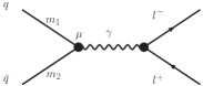
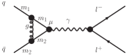
Figure 6: Leading order and vertex correction processes to DY production. Note that only the interference of the two processes contributes at NLO.

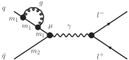
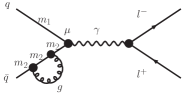
Figure 7: Wave function renormalization processes for DY production at NLO.

It is important to note at this point that our initial state quarks have different masses $m_{1}$ and $m_{2}$ when we evaluate the matrix elements of the loop correction and the bremsstrahlung diagrams, just as in the LO calculation in Sec. II.3. However, we keep the quark mass fixed at the quark-gluon vertex, see Figs. 6, 7 and 8. This guarantees that also in the strong sector gauge invariance is preserved, as we show in Appendix A. For the same reason all gluons are treated as massless.

In the case of gluon Compton scattering we keep the quark mass fixed at every vertex, see Fig. 9, for the following reasons: In principle the final state quark is supposed to be “free” and thus one would assign to it a mass $m_{1}=0$. To preserve gauge invariance the quark mass at the gluon vertex must not change and thus the exchange quark in the right diagram in Fig. 9 would have to be also massless. This, however, immediately generates an infrared (IR) divergence, as will be illustrated in Sec. III.4. Therefore, we assign a mass $m_{1}$ to the entire quark line.

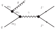
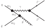
Figure 8: Gluon bremsstrahlung processes for DY production at NLO.

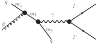
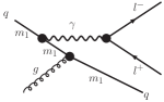
Figure 9: Gluon Compton scattering processes for DY production at NLO.

III.1 Vertex correction

III.1.1 Form factors

The vertex correction process of Fig. 6 together with the wave function renormalization of Fig. 7 modifies the bare quark-photon vertex:

$$\gamma^{\mu}\rightarrow\Gamma^{\mu}=\gamma^{\mu}+\delta\Gamma^{\mu}(\alpha_{s})+O(\alpha_{s}^{2})\ .$$ (80)

From general principles one now can decompose the correction into

$$\delta\Gamma^{\mu}=A\cdot\gamma^{\mu}+B\cdot(p_{1}-p_{2})^{\mu}\ +C\cdot(p_{1}+p_{2})^{\mu},$$ (81)

where $A$, $B$ and $C$ are functions of $q^{2}$, $m_{1}$ and $m_{2}$. However, in DY pair-production the term $(p_{1}+p_{2})^{\mu}$ does not contribute, as we show in detail in Appendix A.1. Therefore, from now on we neglect this term.

The Gordon identity Peskin and Schroeder (1995) for the case of different masses $m_{1}$ and $m_{2}$ reads:

$$\bar{v}(p_{2},m_{2})\gamma^{\mu}u(p_{1},m_{1})=$$

$$\bar{v}(p_{2},m_{2})\left(\frac{(p_{1}-p_{2})^{\mu}}{m_{1}+m_{2}}+\frac{i\sigma^{\mu\nu}q_{\nu}}{m_{1}+m_{2}}\right)u(p_{1},m_{1})$$ (82)

and thus we find:

$$\Gamma^{\mu}=\gamma^{\mu}\cdot\left(1+A+(m_{1}+m_{2})B\right)+\frac{i\sigma^{\mu\nu}q_{\nu}}{m_{1}+m_{2}}\cdot(-(m_{1}+m_{2})B)\ .$$ (83)

We can now identify the well known form factors $F_{1}$ and $F_{2}$ Peskin and Schroeder (1995):

$$F_{1} =1+A+(m_{1}+m_{2})B\ ,$$ (84)

$$F_{2} =-(m_{1}+m_{2})B\ .$$ (85)

The calculation of $A$ and $B$ is tedious, but straightforward. We will only need the real parts of $A$ and $B$, see Eq. (100):

$$\text{Re}(A)=$$

$$\frac{\alpha_{s}}{4\pi}\cdot\text{Re}\left(-3+\log(1-v^{2})-\frac{1}{2}\left(\log(1-\alpha^{2})+\log(1-(\alpha+\phi)^{2})\right)-\frac{\alpha}{2}\left(\log\frac{\alpha+1}{\alpha-1}+\log\frac{\alpha+\phi+1}{\alpha+\phi-1}\right)-\frac{\phi}{2}\log\frac{\alpha+\phi+1}{\alpha+\phi-1}+I_{1}\right)\ ,$$ (86)

with

$$I_{1}= -1+\frac{\phi}{2}\log\frac{1-v^{2}}{1-v^{2}-2\phi}-\frac{4v^{2}+3\phi+\tau+\frac{\phi^{2}}{2}}{2\alpha+\phi}\left(\log\frac{\alpha-1}{\alpha+1}+\log\frac{\alpha+\phi-1}{\alpha+\phi+1}\right)+2(1+v^{2}+\phi)\cdot I_{3}-2\log(\kappa)+\frac{3}{2}\log\left(\frac{m_{1}^{2}}{m_{2}^{2}}\right)\ ,$$ (87)

$$I_{3}= \frac{1}{2r}\left[\log(\kappa)\log\frac{r+1-\frac{\phi}{2}}{r-1-\frac{\phi}{2}}+\log\frac{v^{2}-1}{2r}\log\frac{r+1-\frac{\phi}{2}}{r-1-\frac{\phi}{2}}-\frac{1}{2}\log^{2}(r+1-\frac{\phi}{2})+\frac{1}{2}\log^{2}(r-1-\frac{\phi}{2})\right.$$

$$\left.+\text{Li}_{2}\left(\frac{r+1-\frac{\phi}{2}}{2r}\right)-\text{Li}_{2}\left(\frac{r-1-\frac{\phi}{2}}{2r}\right)+\log^{2}\left(\sqrt{\frac{1-v^{2}}{1-v^{2}-2\phi}}\right)+\log\left(\sqrt{\frac{1-v^{2}}{1-v^{2}-2\phi}}\right)\log(\kappa)\right]\ ,$$ (88)

$$\text{Re}(B)=\frac{\alpha_{s}}{4\pi}\frac{1}{m_{1}}\cdot\text{Re}\left[\frac{\frac{\tau}{4}(1-\alpha)+\frac{v^{2}-1}{2}}{2\alpha+\phi}\left(\log\frac{\alpha-1}{\alpha+1}+\log\frac{\alpha+\phi-1}{\alpha+\phi+1}\right)-\frac{\tau}{4}\log\frac{\alpha+\phi+1}{\alpha+\phi-1}\right]$$ (89)

and

$$v= \sqrt{1-\frac{4m_{1}^{2}}{q^{2}}}\ ,$$ (90)

$$\tau= (1-v^{2})\cdot\left(1-\frac{m_{2}}{m_{1}}\right)\ ,$$ (91)

$$\phi= \frac{1}{2}\cdot\left(1-\frac{m_{2}^{2}}{m_{1}^{2}}\right)\cdot(1-v^{2})\ ,$$ (92)

$$\alpha= -\frac{\phi}{2}+\sqrt{\phi+v^{2}+\frac{\phi^{2}}{4}}\ ,$$ (93)

$$r= \sqrt{\phi+v^{2}+\frac{\phi^{2}}{4}}\ ,$$ (94)

$$\kappa= \frac{\lambda^{2}}{m_{1}^{2}}\ .$$ (95)

$\text{Li}_{2}$ is the Dilogarithm or Spence function.

We have checked and confirmed that in the limit of equal masses $m_{2}\rightarrow m_{1}$ the well known formula for $F_{1}(q^{2},m^{2})$ Muta (1998); Berends et al. (1973) is recovered. We note that also for unequal masses the ultraviolet (UV) divergences of the loops, displayed in Figs. 6, 7, cancel. This is by virtue of the Ward-Takahashi identities, which are fulfilled at the quark-gluon vertices, since there by construction the mass of the quark does not change. However, for $m_{1}\neq m_{2}$ one finds that gauge invariance is broken at the quark-photon vertex (the full amplitude is gauge invariant, see Appendix A.1). The gauge dependence of the quark-photon vertex results in a finite renormalization of the charge, which cannot be canceled by gauge invariant counterterms. Therefore one finds:

$$\underset{q^{2}\rightarrow 0}{\lim}F_{1}(q^{2},m_{1}^{2},m_{2}^{2})\neq 1\ .$$ (96)

On the other hand, $q^{2}=M^{2}$ sets the hard scale in DY pair production and thus our model should only be applied at reasonably large $q^{2}$. A sensible lower limit would be $q^{2}>1\text{ GeV}^{2}$. Thus we probe $F_{1}$ far away from $q^{2}=0$ and we show in Appendix B that for these physically interesting $q^{2}$ the influence of the renormalized charge is negligible.

III.1.2 Soft gluon divergence

To obtain Eqs. (86-95) we have assigned to the gluon a mass $\lambda$ which serves as an IR regulator in the loop integral. According to the theorems by Kinoshita-Poggio-Quinn Kinoshita (1962); Kinoshita and Ukawa (1976); Poggio and Quinn (1976); Sterman (1976) and Kinoshita-Lee-Nauenberg Kinoshita (1962); Lee and Nauenberg (1964) the (IR) divergence of the loop integral cancels against a similar divergence of the bremsstrahlung processes in Fig. 8. Therefore we will also introduce the same gluon mass $\lambda$ in the calculation of the bremsstrahlung in Sec. III.2 and we will show in Sec. IV.1, that the two divergences actually cancel numerically, as they should.

III.1.3 Interference cross section

The LO partonic cross section can be written as ($M^{2}=q^{2}$)

$$\frac{\textrm{d}\hat{\sigma}_{\text{LO}}}{\textrm{d}M^{2}\textrm{d}t}=\frac{1}{3}\frac{\pi\alpha^{2}}{6M^{3}p_{\textrm{cm}}}\cdot T_{\text{LO}}\cdot\delta(s-M^{2})\,\delta(t-m_{1}^{2})\ ,$$ (97)

where $\frac{1}{3}$ is the color factor and

$$T_{\text{LO}}=\left(-g_{\mu\nu}+\frac{q_{\mu}q_{\nu}}{q^{2}}\right)\cdot\text{Tr}\left[(\not{p}_{2}-m_{2})\gamma^{\mu}(\not{p}_{1}+m_{1})\gamma^{\nu}\right]\ .$$ (98)

From this one easily finds that the cross section of the interference of the LO process and the vertex correction can be written as

$$\frac{\textrm{d}\hat{\sigma}_{\text{VC}}}{\textrm{d}M^{2}\textrm{d}t}=\frac{1}{3}\frac{\pi\alpha^{2}}{6M^{3}p_{\textrm{cm}}}\cdot T_{\text{VC}}\cdot\delta(s-M^{2})\,\delta(t-m_{1}^{2})\ ,$$ (99)

with

$$T_{\text{VC}}= \left(-g_{\mu\nu}+\frac{q_{\mu}q_{\nu}}{q^{2}}\right)$$

$$\times \left(2\,\text{Re}(A)\cdot\text{Tr}\left[(\not{p}_{2}-m_{2})\gamma^{\mu}(\not{p}_{1}+m_{1})\gamma^{\nu}\right]\right.$$

$$\left.\ 2\,\text{Re}(B)\cdot\text{Tr}\left[(\not{p}_{2}-m_{2})\gamma^{\mu}(\not{p}_{1}+m_{1})\right]\cdot(p_{1}-p_{2})^{\nu}\right)\ .$$ (100)

Note that $\textrm{d}\hat{\sigma}_{\text{VC}}$ depends on the gluon mass $\lambda$ of Eq. (95) and so does the cross section for gluon bremsstrahlung of Sec. III.2. Only the sum of the two cross sections is a physically meaningful quantity and thus we will only plot the sum of the two in our results in Sec. IV.

III.1.4 Kinematics

Since the vertex correction shares initial and final states with the LO process, the hadronic cross section of the vertex correction is calculated exactly as described for the LO mass distribution case in Sec. II.3.

III.2 Gluon bremsstrahlung

In the case of gluon bremsstrahlung we assign the same fictitious mass $\lambda$ to the gluon as for the vertex correction process. This ensures the cancellation of the soft gluon divergences, as we will show in Sec. IV. Then the partonic cross section becomes ($E_{g}\geq\lambda$)

$$\frac{\textrm{d}\hat{\sigma}_{\text{B}}}{\textrm{d}M^{2}\textrm{d}t}=\frac{4}{9}\frac{\alpha^{2}\alpha_{s}}{48M^{2}}\cdot\frac{T_{\text{B}}}{sp_{\textrm{cm}}^{2}}\cdot\Theta(E_{g})\ .$$ (101)

Here $\frac{4}{9}$ is the color factor and $T_{B}$ is given by

$$T_{\text{B}}=\left(g_{\mu\nu}-\frac{q_{\mu}q_{\nu}}{q^{2}}\right)\cdot\text{Tr}\left[(\not{p}_{2}-m_{2})S^{\alpha\mu}(\not{p}_{1}+m_{1})S^{\nu}_{\ \alpha}\right]$$ (102)

with

$$S^{\alpha\beta}=\gamma^{\alpha}\,\frac{\not{p}_{1}-\not{q}+m_{2}}{(p_{1}-q)^{2}-m_{2}^{2}}\gamma^{\beta}+\gamma^{\beta}\,\frac{\not{q}-\not{p}_{2}+m_{1}}{(p_{2}-q)^{2}-m_{1}^{2}}\gamma^{\alpha}\ .$$ (103)

The calculation of the hadronic cross section basically follows along the same lines as for the LO case in Sec. II.3. Once again one has to remove unphysical solutions for the momentum fractions $x_{i}$, however, the calculation of the phase space is more subtle. The details of this calculation are given in appendix C.1.

III.3 Gluon Compton scattering

For gluon Compton scattering we choose for the initial quark/antiquark to have four-momentum $p_{1}$ and for the gluon to have four-momentum $p_{2}$, thus $m_{2}=0$ since the gluon is real. For the outgoing quark/antiquark we then have $m_{r}=m_{1}$. The partonic cross section then reads ($E_{r}\geq m_{r}$):

$$\frac{\textrm{d}\hat{\sigma}_{\text{C}}}{\textrm{d}M^{2}\textrm{d}t}=\frac{1}{6}\frac{\alpha^{2}\alpha_{s}}{12M^{2}(s-m_{1}^{2})^{2}}\cdot T_{\text{C}}\cdot\Theta(E_{r})\ ,$$ (104)

where $\frac{1}{6}$ is the color factor and $T_{C}$ is given by

$$T_{\text{C}}=\left(g_{\mu\nu}-\frac{q_{\mu}q_{\nu}}{q^{2}}\right)\cdot\text{Tr}\left[(\not{p}_{1}+\not{p}_{2}-\not{q}+m_{1})S^{\mu\alpha}(\not{p}_{1}+m_{1})S_{\alpha}^{\ \nu}\right]$$ (105)

with

$$S^{\alpha\beta}=\gamma^{\alpha}\,\frac{\not{p}_{1}+\not{p}_{2}+m_{1}}{(p_{1}+p_{2})^{2}-m_{1}^{2}}\gamma^{\beta}+\gamma^{\beta}\,\frac{\not{p}_{1}-\not{q}+m_{1}}{(p_{1}-q)^{2}-m_{1}^{2}}\gamma^{\alpha}\ .$$ (106)

The calculation of the hadronic cross section is similar to the case of gluon bremsstrahlung, however, the inherent asymmetry of the initial state (massive quark hits massless gluon) requires additional care. The details can be found in appendix C.3.

III.4 Influence of quark mass distributions on DY $p_{T}$ spectra

As already mentioned in the introduction, massless pQCD calculations of DY pair production at NLO produce divergent $p_{T}$ spectra Gavin et al. (1995). The origin of these IR divergences are twofold: first there is soft gluon emission (bremsstrahlung). This type of soft divergence, however, is not problematic, since it exactly cancels against a divergence in the virtual processes (vertex correction), cf. Sec. III.1.2. Second there is emission (bremsstrahlung) or capture (Compton scattering) of a gluon by a massless participant quark (also called mass or collinear singularity): the $u$-channel exchange quarks in Figs. 8 and 9 can become onshell at $p_{T}=0$ and thus for $m_{1}=m_{2}=0$ the propagators in Eqs. (103,106) produce a non-integrable (in $p_{T}^{2}$) singularity at $p_{T}=0$. To address this problem was one reason for introducing mass distributions for the participating quarks. This procedure aims at smearing out the divergence and so making the $p_{T}$ spectra integrable.

We will illustrate this procedure on the example of the gluon Compton scattering process. In Fig. 10 we compare $p_{T}$ spectra produced by gluon Compton scattering in two different schemes: one calculation with massless quarks and a calculation which includes quark mass distributions. In both cases the quark’s initial transverse momentum is set to zero. It is seen that now indeed a transverse momentum of the dileptons is generated. However, its magnitude is significantly underestimated. One can also see clearly that the rise for $p_{T}\rightarrow 0$ of the calculation with mass distributions is slower than for the calculation with massless quarks. This is a consequence of the effective cut-off, which is introduced by distributing the quark masses. We find that the divergence in $p_{T}$ is softened enough to make the $p_{T}$ spectra integrable.

Figure 10: $p_{T}$ spectrum of gluon Compton scattering obtained from massless and mass distribution approach with initially collinear quarks. The PDFs are the MSTW2008LO68cl set. Data are from E866 binned with $4.2$ GeV $<M<5.2$ GeV, $-0.05<x_{F}<0.15$. Only statistical errors are shown.

III.5 Collinear (mass) singularities and parton distribution functions

As we have just shown, we have regularized the collinear singularities of the NLO processes by introducing quark mass distributions. However, for the calculation of the cross sections we would like to use PDFs as supplied in the literature. But exactly those collinear singularities, that we have just regularized, are commonly absorbed into the definition of the standard PDFs. Thus, to avoid double-counting, in this section we present a subtraction scheme, that leaves us with a consistent cross section to the order of the hard processes we are considering.

To set the stage we first review briefly the introduction of the renormalized PDFs into pQCD. For the DY process this concerns the calculation of $M$ spectra, because the spectra differential in $p_{T}$ are not accessible by pQCD. Since we are interested in the description of fully differential DY spectra by our model, we have to modify the way towards the standard renormalized PDFs. This is outlined in a second subsection.

III.5.1 Collinear singularities in pQCD

If Bjorken-scaling were not violated the PDFs found in deep inelastic scattering were functions of the momentum fraction $x$ only. However, it is well known that the interactions among the quarks and gluons induce scaling violations via processes like gluon bremsstrahlung and gluon quark-antiquark production. To calculate the contributions of these processes to the longitudinal PDFs one has to integrate over the transverse momentum of the emitted particle (quark or gluon) and finds, that they suffer from collinear (or mass) singularities, i.e. they are singular because the quarks are treated as massless. The divergences appear at the boundaries of the transverse momentum integrals (which is why they are called collinear divergences). Thus, one can regulate these divergences by introducing a regulating cut-off $\eta^{2}$ in the transverse momentum integral. In this scheme one can define renormalized longitudinal quark PDFs by absorbing the collinear singularities and the (non-measurable, scaling) bare quark and gluon PDFs, $f_{i}^{0}(x)$ and $g^{0}(x)$, into one function Ellis et al. (1996):

$$f_{i}(x,\mu^{2})$$

$$= f_{i}^{0}(x)+\frac{\alpha_{s}}{2\pi}\int_{x}^{1}\textrm{d}y\ \frac{1}{y}\left\{f_{i}^{0}(y)\left[P_{qq}\left(\frac{x}{y}\right)\log\left(\frac{\mu^{2}}{\eta^{2}}\right)+C^{S}_{q}\left(\frac{x}{y}\right)\right]\right.$$

$$\phantom{f_{i}^{0}(x)+\frac{\alpha_{s}}{2\pi}\int_{x}^{1}\textrm{d}y\ }+\left.g^{0}(y)\left[P_{qg}\left(\frac{x}{y}\right)\log\left(\frac{\mu^{2}}{\eta^{2}}\right)+C^{S}_{g}\left(\frac{x}{y}\right)\right]\right\}\ ,$$ (107)

with the hard scale $\mu^{2}$. The coefficient functions of the divergent logarithms are the splitting functions $P_{qq}$ and $P_{qg}$, which are given below. The functions $C^{\text{S}}_{q}$ and $C^{\text{S}}_{g}$ contain possible finite contributions of the scaling violating processes and the superscript S reminds us of the fact, that these finite contributions depend on the chosen renormalization scheme, since only the divergent contributions actually have to be absorbed into the renormalized PDFs. The splitting functions found in deep inelastic scattering to order $\alpha_{s}$ are given by Ellis et al. (1996)

$$P_{qq}(x) =\frac{4}{3}\left[\frac{1+x^{2}}{\left(1-x\right)_{+}}+\frac{3}{2}\delta\left(1-x\right)\right]\ ,$$ (108)

$$P_{qg}(x) =\frac{1}{2}\left[x^{2}+(1-x)^{2}\right]\ ,$$ (109)

where $\frac{4}{3}$ and $\frac{1}{2}$ are color factors. The plus prescription reads:

$$\int_{0}^{1}\textrm{d}x\frac{f(x)}{\left(1-x\right)_{+}}=\int_{0}^{1}\textrm{d}x\frac{f(x)-f(1)}{1-x}\ ,$$ (110)

where $f$ is a smooth function on $[0,1]$.

Remarkably one finds the same splitting functions when calculating order $\alpha_{s}$ corrections to DY pair production Ellis et al. (1996): $P_{qq}$ collects all the contributions from the processes with $q\bar{q}$ in the initial state, i.e. the vertex correction and gluon bremsstrahlung processes of Figs. 6, 7 and 8. $P_{qg}$ contains the contributions from the gluon Compton scattering processes in Fig. 9. Then the partonic cross section for DY pair production to order $\alpha_{s}$ integrated over the transverse momentum of the DY pair can be written schematically as Ellis et al. (1996)

$$\frac{\textrm{d}\hat{\sigma}}{\textrm{d}M^{2}}=\frac{4\pi\alpha^{2}}{9M^{4}}e_{i}^{2}z\left[\delta\left(1-z\right)+\frac{\alpha_{s}}{2\pi}\left(\mathcal{F}_{q\bar{q}}(z)+\mathcal{F}_{qg}(z)\right)\right]\ ,$$ (111)

for a quark of flavor $i$ and with

$$z=\frac{M^{2}}{\hat{s}}=\frac{M^{2}}{x_{1}x_{2}S}=\frac{\tau}{x_{1}x_{2}}\ ,$$ (112)

where $\sqrt{\hat{s}}$ ($\sqrt{S}$) is the partonic (hadronic) c.m. energy and $x_{1},x_{2}$ the momentum fractions of the quarks. The $\delta$-function in (111) gives just the leading-order contribution and the functions $\mathcal{F}_{q\bar{q}}$ and $\mathcal{F}_{qg}$ give the contributions with initial states consisting of quark-antiquark (vertex correction and gluon bremsstrahlung) and quark-gluon (gluon Compton scattering), respectively:

$$\mathcal{F}_{q\bar{q}}(z) =2P_{qq}(z)\log\left(\frac{M^{2}}{\eta^{2}}\right)+\hat{C}^{\text{S}}_{q}(z)\ ,$$ (113)

$$\mathcal{F}_{qg}(z) =P_{qg}(z)\log\left(\frac{M^{2}}{\eta^{2}}\right)+\hat{C}^{\text{S}}_{g}(z)\ ,$$ (114)

where again the cut-off $\eta^{2}$ was introduced to regulate the transverse momentum integration and where the functions $\hat{C}^{\text{S}}_{q}$ and $\hat{C}^{\text{S}}_{g}$ are again renormalization scheme dependent, finite contributions. In principle one could obtain the hadronic cross section by folding the partonic cross section (111) with the bare parton distributions and summing over all quark flavors:

$$\frac{\textrm{d}\sigma}{\textrm{d}M^{2}}$$

$$= \frac{4\pi\alpha^{2}}{9M^{4}}\sum_{i}e_{i}^{2}\int_{0}^{1}\textrm{d}x_{1}\textrm{d}x_{2}\frac{\tau}{x_{1}x_{2}}\Theta\left(x_{1}x_{2}-\tau\right)$$

$$\times\left\{\left(f_{i}^{0}(x_{1})f_{\bar{i}}^{0}(x_{2})+(f_{i}^{0}\leftrightarrow f^{0}_{\bar{i}})\right)\left[\delta\left(1-z\right)+\frac{\alpha_{s}}{2\pi}\mathcal{F}_{q\bar{q}}(z)\right]\right.$$

$$+\left.\left(g^{0}(x_{1})\left(f_{i}^{0}(x_{2})+f_{\bar{i}}^{0}(x_{2})\right)+(g^{0}\leftrightarrow f^{0}_{i},f^{0}_{\bar{i}})\right)\frac{\alpha_{s}}{2\pi}\mathcal{F}_{qg}(z)\right\}\ .$$ (115)

This cross section cannot be evaluated straigtforwardly, since neither the bare parton distributions are available, nor are $\mathcal{F}_{q\bar{q}}$ and $\mathcal{F}_{qg}$ well defined, since they depend on the arbitrary cut-off $\eta^{2}$. However, we note the following relation for a general function $P$:

$$\int_{0}^{1}\textrm{d}x_{1}\textrm{d}x_{2}\frac{\tau}{x_{1}x_{2}}\Theta\left(x_{1}x_{2}-\tau\right)f_{i}^{0}(x_{1})f_{\bar{i}}^{0}(x_{2})P\left(\frac{\tau}{x_{1}x_{2}}\right)$$

$$= \tau\int_{\tau}^{1}\frac{\textrm{d}x_{1}}{x_{1}}f_{i}^{0}(x_{1})\int_{\frac{\tau}{x_{1}}}^{1}\frac{\textrm{d}x_{2}}{x_{2}}P\left(\frac{\tau}{x_{1}x_{2}}\right)f_{\bar{i}}^{0}(x_{2})$$

$$= \tau\int_{\tau}^{1}\frac{\textrm{d}x_{1}}{x_{1}}f_{i}^{0}(x_{1})\int_{\tau}^{1}\textrm{d}x_{2}\delta\left(x_{2}-\frac{\tau}{x_{1}}\right)\int_{x_{2}}^{1}\frac{\textrm{d}y}{y}P\left(\frac{x_{2}}{y}\right)f_{\bar{i}}^{0}(y)$$

$$= \tau\int_{0}^{1}\textrm{d}x_{1}\textrm{d}x_{2}\textrm{d}z\delta\left(1-z\right)\delta\left(x_{1}x_{2}z-\tau\right)f_{i}^{0}(x_{1})$$

$$\times\int_{x_{2}}^{1}\frac{\textrm{d}y}{y}P\left(\frac{x_{2}}{y}\right)f_{\bar{i}}^{0}(y)\ .$$ (116)

In addition one finds for the product of two renormalized PDFs of the type of Eq. (107)

$$f_{i}(x_{1},M^{2})f_{\bar{i}}(x_{2},M^{2})$$

$$= f_{i}^{0}(x_{1})f_{\bar{i}}^{0}(x_{2})$$

$$+ f_{i}^{0}(x_{1})\frac{\alpha_{s}}{2\pi}\int_{x_{2}}^{1}\textrm{d}y\ \frac{1}{y}\left\{f_{\bar{i}}^{0}(y)\left[P_{qq}\left(\frac{x_{2}}{y}\right)\log\left(\frac{M^{2}}{\eta^{2}}\right)+C^{S}_{q}\left(\frac{x_{2}}{y}\right)\right]\right.$$

$$\phantom{f_{i}^{0}(x_{2})+\frac{\alpha_{s}}{2\pi}\int_{x}^{1}\ \ }+\left.g^{0}(y)\left[P_{qg}\left(\frac{x_{2}}{y}\right)\log\left(\frac{M^{2}}{\eta^{2}}\right)+C^{S}_{g}\left(\frac{x_{2}}{y}\right)\right]\right\}$$

$$+ f_{\bar{i}}^{0}(x_{2})\frac{\alpha_{s}}{2\pi}\int_{x_{1}}^{1}\textrm{d}y\ \frac{1}{y}\left\{f_{i}^{0}(y)\left[P_{qq}\left(\frac{x_{1}}{y}\right)\log\left(\frac{M^{2}}{\eta^{2}}\right)+C^{S}_{q}\left(\frac{x_{1}}{y}\right)\right]\right.$$

$$\phantom{f_{i}^{0}(x_{2})+\frac{\alpha_{s}}{2\pi}\int_{x}^{1}\ \ }+\left.g^{0}(y)\left[P_{qg}\left(\frac{x_{1}}{y}\right)\log\left(\frac{M^{2}}{\eta^{2}}\right)+C^{S}_{g}\left(\frac{x_{1}}{y}\right)\right]\right\}$$

$$+ O\left(\alpha_{s}^{2}\right)\ .$$ (117)

Comparing the last two equations, one finds, that one can express the hadronic cross section (115) in terms of the renormalized PDFs (107). One obtains Ellis et al. (1996)

$$\frac{\textrm{d}\sigma}{\textrm{d}M^{2}}$$

$$= \frac{4\pi\alpha^{2}}{9M^{4}}\tau\sum_{i}e_{i}^{2}\int_{0}^{1}\textrm{d}x_{1}\textrm{d}x_{2}\textrm{d}z\delta\left(x_{1}x_{2}z-\tau\right)$$

$$\times\left\{\left(f_{i}(x_{1},M^{2})f_{\bar{i}}(x_{2},M^{2})+(f_{i}\leftrightarrow f_{\bar{i}})\right)\left[\delta\left(1-z\right)+\frac{\alpha_{s}}{2\pi}\tilde{C}^{\text{S}}_{q}(z)\right]\right.$$

$$+\left[g(x_{1},M^{2})\left(f_{i}(x_{2},M^{2})+f_{\bar{i}}(x_{2},M^{2})\right)\right.$$

$$\phantom{+\ \ }+\left.\left.(g\leftrightarrow f_{i},f_{\bar{i}})\right]\frac{\alpha_{s}}{2\pi}\tilde{C}^{\text{S}}_{g}(z)\right\}\ ,$$ (118)

which is correct to $O(\alpha_{s})$. The collinear divergences and the bare PDFs have been absorbed into the renormalized PDFs. Again there remain scheme-dependent finite contributions $\tilde{C}_{q}$, $\tilde{C}_{g}$.

III.5.2 Collinear singularities in our model

The introduction of the renormalized PDFs gives rise to the famous DGLAP evolution equation which describe successfully the scaling violations Ellis et al. (1996). Clearly for our model we want to inherit this fundamental QCD property. Also from a pragmatic point of view we want to use the standard (renormalized) PDFs from the literature. On the other hand, in the pQCD approach to the DY process the reshuffling of the collinear singularities into the renormalized PDFs is only possible for the $p_{T}$ integrated $M$ spectrum. In our model we also want to describe the DY spectra differential in $p_{T}$. Therefore, we cannot follow the steps outlined in the previous subsection. However, we have an explicit regularization of the collinear singularities. This allows to make contact between the bare and the renormalized PDFs by a kind of backward engineering, which we will describe next.

Since we explicitly take into account all $O(\alpha_{s})$ processes, cf. Secs. III.1-III.3, we now have to ensure that all the $O(\alpha_{s})$ contributions to the cross section, that were absorbed into the renormalized PDFs are subtracted. Otherwise we would double-count the $O(\alpha_{s})$ contributions. Schematically the hadronic cross section for DY pair production to next-to-leading order in $\alpha_{s}$ can be written as

$$\textrm{d}\sigma=\int\sum_{i}e_{i}^{2} \left[\underbrace{\textrm{d}\hat{\sigma}_{\text{LO}}}_{O(\alpha_{s}^{0})=O(1)}f_{i}^{0}\cdot f_{\bar{i}}^{0}+\underbrace{\textrm{d}\hat{\sigma}_{\text{VC+B}}}_{O(\alpha_{s})}\ f_{i}^{0}\cdot f_{\bar{i}}^{0}\right.$$

$$+\left.\underbrace{\textrm{d}\hat{\sigma}_{\text{C}}}_{O(\alpha_{s})}\ g^{0}\cdot(f_{i}^{0}+f_{\bar{i}}^{0})\right]\ ,$$ (119)

with the bare PDFs $f_{i}^{0}$, $g^{0}$. We note that $f_{i}\cdot f_{\bar{i}}=f_{i}^{0}f_{\bar{i}}^{0}+O(\alpha_{s})$ and $g\cdot(f_{i}+f_{\bar{i}})=g^{0}\cdot(f_{i}^{0}+f_{\bar{i}}^{0})+O(\alpha_{s})$, and so to $O(\alpha_{s})$ nothing changes if we replace the bare PDFs multiplying the NLO partonic cross sections:

$$\textrm{d}\sigma=\int\sum_{i}e_{i}^{2} \left[\underbrace{\textrm{d}\hat{\sigma}_{\text{LO}}}_{O(\alpha_{s}^{0})=O(1)}f_{i}^{0}\cdot f_{\bar{i}}^{0}+\underbrace{\textrm{d}\hat{\sigma}_{\text{VC+B}}}_{O(\alpha_{s})}\ f_{i}\cdot f_{\bar{i}}\right.$$

$$+\left.\underbrace{\textrm{d}\hat{\sigma}_{\text{C}}}_{O(\alpha_{s})}\ g\cdot(f_{i}+f_{\bar{i}})\right]+O(\alpha_{s}^{2})\ .$$ (120)

However, if we were to do the same with the LO term, we would get additional $O(\alpha_{s})$ contributions, cf. Eq. (117). How do we subtract these contributions? After all, we cannot calculate the integrals in Eq. (117), since we do not know $\eta$ or the bare PDFs.

In our model we set out to calculate exactly those transverse momentum spectra that were integrated in the derivation of the renormalized PDFs in the pQCD case above. To accomplish this, we have introduced quark mass distributions to handle the collinear divergences that enter the quark PDF in Eq. (107). The important difference between the pQCD approach and our model is, therefore, the following: in pQCD the regulating cut-off $\eta^{2}$ is completely arbitrary and physical results can only be obtained by “absorbing” this arbitrariness into the renormalized PDFs. All the finite and scheme-depedent contributions can be calculated analytically. In our model we know the regulator $\eta$ in (107), it is nothing but our quark mass $m$ (or better $m^{2}$). However, we do not know the finite contributions $C^{\text{S}}_{q,g}$ in our model. To estimate them, we introduce two new parameters $\kappa_{q}$ and $\kappa_{g}$, so that the functions $\mathcal{F}_{q\bar{q}}$ and $\mathcal{F}_{qg}$ become:

$$\mathcal{F}^{m}_{q\bar{q}}(z) =2P_{qq}(z)\log\left(\frac{M^{2}}{\kappa_{q}^{2}m^{2}}\right)\ ,$$ (121)

$$\mathcal{F}^{m}_{qg}(z) =P_{qg}(z)\log\left(\frac{M^{2}}{\kappa_{g}^{2}m^{2}}\right)\ .$$ (122)

Then we can rewrite the renormalized PDFs in Eq. (117) as

$$f_{i}(x_{1},M^{2})f_{\bar{i}}(x_{2},M^{2})$$

$$= f_{i}^{0}(x_{1})f_{\bar{i}}^{0}(x_{2})$$

$$+ f_{i}^{0}(x_{1})\frac{\alpha_{s}}{2\pi}\int_{x_{2}}^{1}\textrm{d}y\ \frac{1}{y}\left\{f_{\bar{i}}^{0}(y)\left[P_{qq}\left(\frac{x_{2}}{y}\right)\log\left(\frac{M^{2}}{\kappa_{q}^{2}m^{2}}\right)\right]\right.$$

$$\phantom{f_{i}^{0}(x_{2})+\frac{\alpha_{s}}{2\pi}\int_{x}^{1}\ \ }+\left.g^{0}(y)\left[P_{qg}\left(\frac{x_{2}}{y}\right)\log\left(\frac{M^{2}}{\kappa_{g}^{2}m^{2}}\right)\right]\right\}$$

$$+ f_{\bar{i}}^{0}(x_{2})\frac{\alpha_{s}}{2\pi}\int_{x_{1}}^{1}\textrm{d}y\ \frac{1}{y}\left\{f_{i}^{0}(y)\left[P_{qq}\left(\frac{x_{1}}{y}\right)\log\left(\frac{M^{2}}{\kappa_{q}^{2}m^{2}}\right)\right]\right.$$

$$\phantom{f_{i}^{0}(x_{2})+\frac{\alpha_{s}}{2\pi}\int_{x}^{1}\ \ }+\left.g^{0}(y)\left[P_{qg}\left(\frac{x_{1}}{y}\right)\log\left(\frac{M^{2}}{\kappa_{g}^{2}m^{2}}\right)\right]\right\}$$

$$+ O\left(\alpha_{s}^{2}\right)\ .$$ (123)

Solving for the product of the bare PDFs gives

$$f_{i}^{0}(x_{1})f_{\bar{i}}^{0}(x_{2})$$

$$= f_{i}(x_{1},M^{2})f_{\bar{i}}(x_{2},M^{2})$$

$$- f_{i}^{0}(x_{1})\frac{\alpha_{s}}{2\pi}\int_{x_{2}}^{1}\textrm{d}y\ \frac{1}{y}\left\{f_{\bar{i}}^{0}(y)\left[P_{qq}\left(\frac{x_{2}}{y}\right)\log\left(\frac{M^{2}}{\kappa_{q}^{2}m^{2}}\right)\right]\right.$$

$$\phantom{f_{i}^{0}(x_{2})+\frac{\alpha_{s}}{2\pi}\int_{x}^{1}\ \ }+\left.g^{0}(y)\left[P_{qg}\left(\frac{x_{2}}{y}\right)\log\left(\frac{M^{2}}{\kappa_{g}^{2}m^{2}}\right)\right]\right\}$$

$$- f_{\bar{i}}^{0}(x_{2})\frac{\alpha_{s}}{2\pi}\int_{x_{1}}^{1}\textrm{d}y\ \frac{1}{y}\left\{f_{i}^{0}(y)\left[P_{qq}\left(\frac{x_{1}}{y}\right)\log\left(\frac{M^{2}}{\kappa_{q}^{2}m^{2}}\right)\right]\right.$$

$$\phantom{f_{i}^{0}(x_{2})+\frac{\alpha_{s}}{2\pi}\int_{x}^{1}\ \ }+\left.g^{0}(y)\left[P_{qg}\left(\frac{x_{1}}{y}\right)\log\left(\frac{M^{2}}{\kappa_{g}^{2}m^{2}}\right)\right]\right\}$$

$$+ O\left(\alpha_{s}^{2}\right)\ .$$ (124)

On the right hand side we can replace all the bare PDFs by their renormalized version, since all additional corrections introduced by this procedure are $O(\alpha_{s}^{2})$:

$$f_{i}^{0}(x_{1})f_{\bar{i}}^{0}(x_{2})$$

$$= f_{i}(x_{1},M^{2})f_{\bar{i}}(x_{2},M^{2})$$

$$- f_{i}(x_{1},M^{2})\frac{\alpha_{s}}{2\pi}\int_{x_{2}}^{1}\textrm{d}y\ \frac{1}{y}\left\{f_{\bar{i}}(y,M^{2})\left[P_{qq}\left(\frac{x_{2}}{y}\right)\log\left(\frac{M^{2}}{\kappa_{q}^{2}m^{2}}\right)\right]\right.$$

$$\phantom{f_{i}^{0}(x_{2})+\frac{\alpha_{s}}{2\pi}\int_{x}^{1}\ \ }+\left.g(y,M^{2})\left[P_{qg}\left(\frac{x_{2}}{y}\right)\log\left(\frac{M^{2}}{\kappa_{g}^{2}m^{2}}\right)\right]\right\}$$

$$- f_{\bar{i}}(x_{2},M^{2})\frac{\alpha_{s}}{2\pi}\int_{x_{1}}^{1}\textrm{d}y\ \frac{1}{y}\left\{f_{i}(y,M^{2})\left[P_{qq}\left(\frac{x_{1}}{y}\right)\log\left(\frac{M^{2}}{\kappa_{q}^{2}m^{2}}\right)\right]\right.$$

$$\phantom{f_{i}^{0}(x_{2})+\frac{\alpha_{s}}{2\pi}\int_{x}^{1}\ \ }+\left.g(y,M^{2})\left[P_{qg}\left(\frac{x_{1}}{y}\right)\log\left(\frac{M^{2}}{\kappa_{g}^{2}m^{2}}\right)\right]\right\}$$

$$+ O\left(\alpha_{s}^{2}\right)\ .$$ (125)

We define

$$f_{i}^{\text{sub}}(x,M^{2}) =\frac{\alpha_{s}}{2\pi}\int_{x}^{1}\textrm{d}y\ \frac{1}{y}f_{i}(y,M^{2})P_{qq}\left(\frac{x}{y}\right)\log\left(\frac{M^{2}}{\kappa_{q}^{2}m^{2}}\right)\ ,$$

$$g^{\text{sub}}(x,M^{2}) =\frac{\alpha_{s}}{2\pi}\int_{x}^{1}\textrm{d}y\ \frac{1}{y}g(y,M^{2})P_{qg}\left(\frac{x}{y}\right)\log\left(\frac{M^{2}}{\kappa_{g}^{2}m^{2}}\right)\ ,$$ (126)

and so we find

$$f_{i}^{0}(x_{1})f_{\bar{i}}^{0}(x_{2})$$

$$= f_{i}(x_{1},M^{2})f_{\bar{i}}(x_{2},M^{2})$$

$$- f_{i}(x_{1},M^{2})f_{\bar{i}}^{\text{sub}}(x_{2},M^{2})-f_{i}(x_{1},M^{2})g^{\text{sub}}(x_{2},M^{2})$$

$$- f_{\bar{i}}(x_{2},M^{2})f_{i}^{\text{sub}}(x_{1},M^{2})-f_{\bar{i}}(x_{2},M^{2})g^{\text{sub}}(x_{1},M^{2})$$

$$+ O\left(\alpha_{s}^{2}\right)\ .$$ (127)

In this scheme the hadronic cross section (120) becomes

$$\textrm{d}\sigma= \int\sum_{i}e_{i}^{2}\left[\textrm{d}\hat{\sigma}_{\text{LO}}f_{i}\cdot f_{\bar{i}}\right.$$

$$-\textrm{d}\hat{\sigma}_{\text{LO}}\left(f_{i}\cdot f^{\text{sub}}_{\bar{i}}+f^{\text{sub}}_{i}\cdot f_{\bar{i}}\right)+\textrm{d}\hat{\sigma}_{\text{VC+B}}\ f_{i}\cdot f_{\bar{i}}$$

$$\left.-\textrm{d}\hat{\sigma}_{\text{LO}}\left(f_{i}\cdot g^{\text{sub}}+f_{\bar{i}}\cdot g^{\text{sub}}\right)+\textrm{d}\hat{\sigma}_{\text{C}}\ g\cdot(f_{i}+f_{\bar{i}})\right]$$

$$+O(\alpha_{s}^{2})\ .$$ (128)

From now on, we label the different contributions to the cross section as sketched in the following:

$$\textrm{d}\sigma_{\text{LO}}=\int\sum_{i}e_{i}^{2} \textrm{d}\hat{\sigma}_{\text{LO}}f_{i}\cdot f_{\bar{i}}\ ,$$ (129)

$$\textrm{d}\sigma_{q\bar{q}}=\int\sum_{i}e_{i}^{2} \textrm{d}\hat{\sigma}_{\text{VC+B}}\ f_{i}\cdot f_{\bar{i}}-\textrm{d}\hat{\sigma}_{\text{LO}}\left(f_{i}\cdot f^{\text{sub}}_{\bar{i}}+f^{\text{sub}}_{i}\cdot f_{\bar{i}}\right)\ ,$$ (130)

$$\textrm{d}\sigma_{qg}=\int\sum_{i}e_{i}^{2} \textrm{d}\hat{\sigma}_{\text{C}}\ g\cdot(f_{i}+f_{\bar{i}})$$

$$- \textrm{d}\hat{\sigma}_{\text{LO}}\left(f_{i}\cdot g^{\text{sub}}+f_{\bar{i}}\cdot g^{\text{sub}}\right)\ .$$ (131)

In Eqs. (130) and (131) we subtract now precisely those $O(\alpha_{s})$ contributions which were absorbed before into the renormalized PDFs. Thus, by this procedure we have produced in our model a consistent cross section to $O(\alpha_{s})$. Indeed, we have checked explicitly that the collinear divergences which appear in $\textrm{d}\sigma_{\text{VC+B}}$, if the quark masses are sent to zero, cancel the corresponding divergence of $f_{i}^{\text{sub}}$ as given in Eq. (126). The same is true for $\textrm{d}\sigma_{\text{C}}$ and $g^{\text{sub}}$. Thus the expressions (130) and (131) remain finite for vanishing quark masses.

For the calculation of our results in Sec. IV we will use Eqs. (129)-(131). The quantities which enter are, on the one hand, the standard PDFs which we can take from the literature, and, on the other hand, the parameters $\kappa_{q}$ and $\kappa_{g}$ which appear in Eq. (126). We recall that these parameters introduced in Eqs. (121) and (122) correspond to finite, i.e. infrared safe, contributions which appear, e.g., as $\hat{C}^{S}_{q,g}$ in Eqs. (113) and (114). We will vary the parameters $\kappa_{q}$ and $\kappa_{g}$ around natural values (i.e. around 1), to estimate these finite contributions.

III.6 Initial transverse momentum distributions

Even in the mass distribution approach at NLO we find that the $p_{T}$ data are heavily underestimated. Therefore, we have also introduced parton initial transverse momentum distributions for the NLO processes, just as we did at LO in Sec. II.2. Taking into account these distributions we obtain a good description of measured cross sections without $K$ factors, as we will show in Sec. IV.

IV Results

In this section we present our combined results of the LO and NLO calculations of Secs. II and III. Since one of our main goals is to gain access to the DY $p_{T}$ spectra, we compare our model with data on $p_{T}$ spectra from different experiments. Most of these experiments were done in proton-nucleus collisions. However, the recent E866 experiment Webb et al. (2003); Webb (2003) measured pp collisions and we will begin to fix the parameters of our model at the data for this more elementary reaction in Sec. IV.1. Using the fixed parameters we compare our results to data for different pp and pA experiments in Secs. IV.2-IV.6. In Sec. IV.7 we study our results for an antiproton-nucleus experiment ($\overline{\text{p}}$N) (E537), which is useful, since one of our aims is to make predictions for DY pair production at $\overline{\text{P}}$ANDA, which will measure antiproton-proton ($\overline{\text{p}}$p) collisions. These predictions can be found in Sec. IV.8.

Our model has effectively four parameters: The width of the initial parton transverse momentum distribution, represented by $D$, the width $\Gamma$ of the quark mass distribution (spectral function) and the two subtraction constants $\kappa_{q}$ and $\kappa_{g}$ which estimate the finite contributions which were absorbed into the PDFs. We will vary $\kappa_{q}$ and $\kappa_{g}$ in a natural range $\frac{1}{2}\dots 2$. The gluon mass $\lambda$ is not really a parameter but a numerical necessity and we will explore its influence on our calculations in Sec. IV.1. In addition our model utilizes standard parton distribution functions. These are calculated by several different groups, for example Martin et al. (2009); Gluck et al. (2008), and they are not unique. We will show results obtained with different leading order PDFs to get an estimate for the theoretical uncertainty. Once again we employ PDFs available through the LHAPDF library, version 5.8.4 Whalley et al. (2005).

At this point we note two things: first, the divergence of the NLO processes near $p_{T}=0$ can also be cured by choosing a finite and fixed quark mass. However it is much more natural to assume a broad mass distribution, since the nucleon is composed of strongly interacting partons; we will show below, that we can describe the experimental data quantitatively well assuming broad quark mass distributions. Second, in principle we could have chosen different transverse momentum and mass distributions for valence quarks, sea quarks and gluons (only transverse momentum in this case). We have not done so for two reasons: on the one hand this would have forced us to introduce additional parameters, while one is of course always inclined to keep the number of parameters as small as possible. On the other hand, as one will see in the results, the data do not require additional modelling. Thus we always use the same distributions from Sec. II.4 for all quarks and gluons (again no mass distributions for the latter).

IV.1 E866 - $p_{T}$ spectrum

In this section we present the results of our full model. The data are from E866 Webb (2003); Webb et al. (2003) for pp collisions at $S=1500\text{ GeV}^{2}$.

Figure 11: $p_{T}$ spectrum obtained from our full model with different values of $D$. Everywhere $\Gamma=0.2$ GeV, $\lambda=5$ MeV, $\kappa_{q}=1$ and $\kappa_{g}=2$. The PDFs are the MSTW2008LO68cl set. Data are from E866 binned with $4.2$ GeV $<M<5.2$ GeV, $-0.05<x_{F}<0.15$. Only statistical errors are shown.

First we want to stress, that the calculation in our full model reproduces measured DY $p_{T}$ spectra without the need for a $K$ factor, see for example Fig. 14. In order to better understand the parameter dependence of our model, in the following we explore the parameter space. The details of how we obtain the presented cross sections were given in Sec. II.5.1. First we show several plots, in which we vary only one parameter and keep the others fixed.

In Fig. 11 we plot the results of our full NLO model for different $D$. As one can see for $D$ around $0.45$ GeV, which corresponds to an average squared initial quark transverse momentum $\langle k_{T}^{2}\rangle=(0.9)^{2}\text{ GeV}^{2}$, the data are reproduced quite well. Obviously, $D$ determines the shape of the $p_{T}$ spectra.

Figure 12: $p_{T}$ spectrum obtained from our full model with different values of $\Gamma$. Everywhere $D=0.45$ GeV, $\lambda=5$ MeV, $\kappa_{q}=1$ and $\kappa_{g}=2$. The PDFs are the MSTW2008LO68cl set. Note that the curves for $\Gamma\geq 0.2$ GeV are on top of each other. Data are from E866 binned with $4.2\text{ GeV }<M<5.2$ GeV, $-0.05<x_{F}<0.15$. Only statistical errors are shown.

In Fig. 12 we show results for different $\Gamma$. The results for several values of $\Gamma$ all agree very well with each other and at the same time reproduce the data quite well. Thus at E866 energies our model appears to be rather insensitive to changes of $\Gamma$ over a wide range.

Figure 13: $p_{T}$ spectrum obtained from our full model with different values of $\lambda$. Everywhere $D=0.45$ GeV, $\Gamma=0.2$ GeV, $\kappa_{q}=1$ and $\kappa_{g}=2$. The PDFs are the MSTW2008LO68cl set. Note that the curves for $\lambda\leq 5$ MeV are on top of each other. Data are from E866 binned with $4.2$ GeV $<M<5.2$ GeV, $-0.05<x_{F}<0.15$. Only statistical errors are shown.

Remember that the gluon mass $\lambda$ is introduced to regulate divergences that occur when the gluons become very soft. In the limit of $\lambda\rightarrow 0$ these divergences of the bremsstrahlung and the vertex correction processes should exactly cancel. Therefore, it is sensible to choose $\lambda$ as small as numerically feasible. Results for different choices of the gluon mass $\lambda$ are shown in Fig. 13. While the results for $\lambda=100,250$ MeV are still visibly larger than the results for $5$ and $0.5$ MeV, the latter two agree very well with each other. Thus the calculated cross section appears to converge in the $\lambda\rightarrow 0$ limit. Therefore, we chose $\lambda=5$ MeV for the calculation of all the following results.

Figure 14: $p_{T}$ spectrum obtained from our full model with different PDF sets. Everywhere $D=0.45$ GeV, $\Gamma=0.2$ GeV, $\lambda=5$ MeV, $\kappa_{q}=1$ and $\kappa_{g}=2$. Data are from E866 binned with $4.2$ GeV $<M<5.2$ GeV, $-0.05<x_{F}<0.15$. Only statistical errors are shown.

We show an example of the influence of different parton distribution functions in Fig. 14. The results with the MSTW2008LO68cl Martin et al. (2009) and GJR08lo Gluck et al. (2008) sets agree quite well with each other, with only small deviations. This is an illustration of the uncertainties induced by the different integrated parton distributions.

Figure 15: $p_{T}$ spectrum obtained from our full model with different values of the subtraction parameter $\kappa_{q}$. Everywhere $D=0.45$ GeV, $\Gamma=0.2$ GeV, $\lambda=5$ MeV and $\kappa_{g}=2$. The PDFs are the MSTW2008LO68cl set. Data are from E866 binned with $4.2$ GeV $<M<5.2$ GeV, $-0.05<x_{F}<0.15$. Only statistical errors are shown.

Figure 16: $p_{T}$ spectrum obtained from our full model with different values of the subtraction parameter $\kappa_{g}$. Everywhere $D=0.45$ GeV, $\Gamma=0.2$ GeV, $\lambda=5$ MeV and $\kappa_{q}=1$. The PDFs are the MSTW2008LO68cl set. Data are from E866 binned with $4.2$ GeV $<M<5.2$ GeV, $-0.05<x_{F}<0.15$. Only statistical errors are shown.

To determine the subtraction parameters $\kappa_{q}$ and $\kappa_{g}$ we explore the dependence of the cross section on these two parameters in Figs. 15 and 16. In the range of natural choices ($\kappa_{q},\kappa_{g}=\frac{1}{2}\dots 2$) we find, that with $\kappa_{q}=1$ and $\kappa_{g}=2$ the data are desribed rather well. Although Fig. 15 would indicate a better fit for smaller $\kappa_{q}$, we stick to $\kappa_{q}=1$, since for this value the slope of the $M$ spectra fits also very well, as we show for example in Sec. IV.4.

Figure 17: $p_{T}$ spectrum obtained from our model decomposed into the different contributions as described at the end of Sec. III.5. Note that we plot the negative quark-gluon contribution. Everywhere $D=0.45$ GeV, $\Gamma=0.2$ GeV, $\lambda=5$ MeV, $\kappa_{q}=1$ and $\kappa_{g}=2$. The PDFs are the MSTW2008LO68cl set. Data are from E866 binned with $4.2$ GeV $<M<5.2$ GeV, $-0.05<x_{F}<0.15$. Only statistical errors are shown.

In Fig. 17 the cross sections of the different contributions to the full result are plotted individually. The definition of the LO, quark-antiquark ($q\bar{q}$) and quark-gluon (qg) contributions is given at the end of Sec. III.5. Note that the sum of the LO contribution and the $q\bar{q}$ corrections make up most of the cross section. The contribution of the $qg$ correction is relatively small and negative for not too large $p_{T}$.

Fig. 18 shows a comparison of the results of our model with the results of a PYTHIA event generator calculation. For this specific plot PYTHIA version 6.225 Sjostrand et al. (2001) with CTEQ5L PDFs Lai et al. (2000) is used and the results are scaled up by a factor $K=2$. The comparison with the experimental data suggests a good fit of the shape of the spectrum for a value of $\langle k_{T}^{2}\rangle=(0.8\text{ GeV})^{2}$ in PYTHIA (internal parameter $\text{PARP(91)}=0.8$). For our value of $D$ we get $\langle k_{T}^{2}\rangle=(2D)^{2}=(0.9\text{ GeV})^{2}$. Although the PYTHIA parameter is obviously intended to have the same meaning as our definition for the average initial transverse momentum, the complex internal treatment of the interaction in the PYTHIA code leads to some numerical mismatch with our implementation.

Figure 18: $p_{T}$ spectrum comparison of PYTHIA results with our full model. For the PYTHIA calculations version 6.225 with CTEQ5L PDFs were used. The PYTHIA result is plotted for two different values of the average initial $k_{T}^{2}$ and multiplied by a factor $K=2$. Our model was calculated with $D=0.45$ GeV, $\Gamma=0.2$ GeV, $\lambda=5$ MeV, $\kappa_{q}=1$, $\kappa_{g}=2$ and MSTW2008LO68cl PDF set. Data are from E866 binned with $4.2$ GeV $<M<5.2$ GeV, $-0.05<x_{F}<0.15$. Only statistical errors are shown.

For comparison we show our results for a different $M$ bin in Fig. 19. With the parameters determined above our full model reproduces the measured spectrum very well. In contrast to the LO approach of Sec. II we do not need a $K$ factor to describe the absolute height of the spectrum. At the same time the width $D$ of the intrinsic (non-perturbative) $k_{T}$ distributions changes only little ($D=0.5$ GeV vs. $D=0.45$ GeV) when passing from the LO to the NLO calculation. Note, however, that Fig. 17 indicates, that at least the results for the $q\bar{q}$ corrections deviate from a Gaussian behavior at $p_{T}\geq 3$ GeV. Thus the contributions of some of the hard NLO processes are only significant in the high (perturbative) $p_{T}$ region. Therefore, to describe the low $p_{T}$ regime at NLO one still requires almost the same non-perturbative input for the intrinsic parton $k_{T}$, i.e., only little transverse momentum is generated dynamically and the width parameter $D$ does not change considerably.

Figure 19: $p_{T}$ spectrum obtained from our full model. Everywhere $D=0.45$ GeV, $\Gamma=0.2$ GeV, $\lambda=5$ MeV, $\kappa_{q}=1$ and $\kappa_{g}=2$. The PDFs are the MSTW2008LO68cl set. Data are from E866 binned with $7.2$ GeV $<M<8.7$ GeV, $-0.05<x_{F}<0.15$. Only statistical errors are shown.

IV.2 E866 - $M$ spectrum

In this section we compare our results with the measured $M$ spectrum from E866, which are basically the $p_{T}$ spectra integrated over $p_{T}$. The double-differential cross section is given by the E866 collaboration as

$$M^{3}\frac{\textrm{d}\sigma}{\textrm{d}M\textrm{d}x_{F}}\ .$$ (132)

Again the data are given in several bins of $M$ and $x_{F}$ and for every datapoint the average values $\left<M\right>$ and $\left<x_{F}\right>$ are provided. For the different contributions in our model we calculate the quantity of Eq. (132) by integrating over $p_{T}^{2}$ for every datapoint using these averaged values:

$$M^{3}\frac{\textrm{d}\sigma}{\textrm{d}M\textrm{d}x_{F}}\rightarrow\left<M\right>^{3}\int_{0}^{(p_{T})^{2}_{\textrm{max}}}\textrm{d}p_{T}^{2}\frac{\textrm{d}\sigma}{\textrm{d}M\textrm{d}x_{F}\textrm{d}p_{T}^{2}}$$

$$=\left<M\right>^{3}\int_{0}^{(p_{T})^{2}_{\textrm{max}}}\textrm{d}p_{T}^{2}\ 2\left<M\right>\frac{\textrm{d}\sigma}{\textrm{d}M^{2}\textrm{d}x_{F}\textrm{d}p_{T}^{2}}\left(\left<M\right>,\left<x_{F}\right>\right)\ .$$ (133)

The maximal possible $p_{T}$ is determined by the kinematics to

$$P_{1}+P_{2} =q+X$$ (134)

$$\Rightarrow(P_{1}+P_{2}-q)^{2} =X^{2}=M_{R}^{2}$$ (135)

$$\Rightarrow S+M^{2}-M_{R}^{2} =2\ (P_{1}+P_{2})\ q$$

$$=2\sqrt{S}E$$

$$=2\sqrt{S}\sqrt{M^{2}+(p_{T})^{2}_{\textrm{max}}+x_{F}^{2}(q_{z})_{\text{max}}^{2}}$$ (136)

$$\Rightarrow E^{2} =M^{2}+(p_{T})^{2}_{\textrm{max}}+x_{F}^{2}(q_{z})_{\text{max}}^{2}$$ (137)

$$=\frac{(S+M^{2}-M_{R}^{2})^{2}}{4S}$$ (138)

$$\Rightarrow(p_{T})^{2}_{\textrm{max}} =\frac{(S+M^{2}-M_{R}^{2})^{2}}{4S}-M^{2}-x_{F}^{2}(q_{z})_{\text{max}}^{2}\ ,$$ (139)

where $M_{R}^{2}$ is the minimal invariant mass of the undetected remnants. For pp and pn collisions we choose a value of $M_{R}=2m_{N}$ and for $\overline{\text{p}}$p a value of $M_{R}=1.1$ GeV, which can be interpreted as two times a diquark mass. Note that at c.m. energies of $\sqrt{S}\approx 15.3$ GeV (E537), $\sqrt{S}\approx 27.4$ GeV (E288, E439) and $\sqrt{S}\approx 38.8$ GeV (E605, E772, E866) we are not really sensitive to these values if they stay at or below a few GeV.

In Fig. 20 we compare our result for the double differential cross section to the data from E866. The slope and absolute height of the curve agree with the data quite well. However, since here the experimental error bars are rather large, we will make comparisons to $M$ spectra from other experiments in Secs. IV.4 and IV.6 to test our model further.

Figure 20: $M$ spectrum obtained from our full model. Everywhere $D=0.45$ GeV, $\Gamma=0.2$ GeV, $\lambda=5$ MeV, $\kappa_{q}=1$ and $\kappa_{g}=2$. The PDFs are the MSTW2008LO68cl set. Data are from E866 binned with $-0.05<x_{F}<0.05$. Only statistical errors shown.

IV.3 E772

Experiment E772 McGaughey et al. (1994) measured dimuon production in pd collisions at $S\approx 1500$ GeV². For the calculation of the triple differential cross section we again use Eq. (76) and for the average values of $M$ and $x_{F}$ we use the center of the $M$ and $x_{F}$ bins. Since the experiment was done on deuterium we have calculated pp and pn cross sections and then averaged.

Figure 21: $p_{T}$ spectrum obtained from our full model with different PDF sets. Everywhere $D=0.45$ GeV, $\Gamma=0.2$ GeV, $\lambda=5$ MeV, $\kappa_{q}=1$ and $\kappa_{g}=2$. Data are from E772 binned with $5$ GeV $<M<6$ GeV, $0.1<x_{F}<0.3$. Only statistical errors are shown.

In Figs. 21 and 22 we compare the results of our full model with different PDF sets to triple differential data from E772 in different $M$ bins. Agreement is again quite well, however, the shape of the spectrum seems to favor a slightly smaller value for $D$, which would enhance the spectrum near $p_{T}=0$. Nevertheless, we have chosen $D=0.45$ GeV, since this value allows us to describe the data from several different experiments with only minor deviations.

Figure 22: $p_{T}$ spectrum obtained from our full model with different PDF sets. Everywhere $D=0.45$ GeV, $\Gamma=0.2$ GeV, $\lambda=5$ MeV, $\kappa_{q}=1$ and $\kappa_{g}=2$. Data are from E772 binned with $7$ GeV $<M<8$ GeV, $0.1<x_{F}<0.3$. Only statistical errors are shown.

IV.4 E605

Experiment E605 Moreno et al. (1991) measured dimuon production in pCu collisions at $S\approx 1500$ GeV². For the calculation of the triple differential cross section we again use Eq. (76) and for the average value of $M$ we use the center of the $M$ bin. For the $p_{T}$ spectrum E605 gives $x_{F}=0.1$. For the double differential cross section we use Eq. (133). Since the experiment was done on copper we have calculated pp and pn cross sections and then averaged (29 protons and 34 neutrons).

Figure 23: $p_{T}$ spectrum obtained from our full model with different PDF sets. Everywhere $D=0.45$ GeV, $\Gamma=0.2$ GeV, $\lambda=5$ MeV, $\kappa_{q}=1$ and $\kappa_{g}=2$. Data are from E605 binned with $7$ GeV $<M<8$ GeV, $x_{F}=0.1$. Only statistical errors are shown.

In Fig. 23 we compare the results of our full model with different PDF sets to triple differential data from E605. Here the shape of the spectrum confirms our chosen value for $D$ and the overall agreement is good.

Figure 24: $M$ spectrum obtained from our full model. Everywhere $D=0.45$ GeV, $\Gamma=0.2$ GeV, $\lambda=5$ MeV, $\kappa_{q}=1$ and $\kappa_{g}=2$. Data are from E605 with $x_{F}=0.125$. Only statistical errors shown.

In Fig. 24 we plot our result with different PDF sets for the double differential cross section together with the data from E605. Again agreement is quite good over the entire range of $M$.

IV.5 E288

Experiment E288 Ito et al. (1981) measured dimuon production in pA collisions at $S\approx 750$ GeV². For the calculation of the triple differential cross section we again use Eq. (76) and for the average value of $M$ we use the center of the $M$ bin. For the $p_{T}$ spectrum E288 gives for the rapidity $y=0.03$ and we thus chose $x_{F}=0$ for our calculation. The experiment was done on different nuclei and only data averaged over the results from these nuclei have been presented. Therefore, we have calculated pp cross sections only.

Figure 25: $p_{T}$ spectrum obtained from our full model with different PDF sets. Everywhere $D=0.45$ GeV, $\Gamma=0.2$ GeV, $\lambda=5$ MeV, $\kappa_{q}=1$ and $\kappa_{g}=2$. Data are from E288 binned with $7$ GeV $<M<8$ GeV, $y=0.03$, we have chosen $x_{F}=0$ in our calculation. Only statistical errors are shown.

In Fig. 25 we compare the results of our full model with different PDF sets to the triple differential data from E288. Again the agreement with the data is good and confirms our choice of parameters.

IV.6 E439

Figure 26: $M$ spectrum obtained from our full model with different PDF sets. Everywhere $D=0.45$ GeV, $\Gamma=0.2$ GeV, $\lambda=5$ MeV, $\kappa_{q}=1$ and $\kappa_{g}=2$. Data are from E439 with $x_{F}^{\prime}=0.1$. Only statistical errors are shown.

The details of experiment E439 and how we calculate the cross section are given in Sec. II.5.2. In Fig. 26 we compare our results for the double differential cross section with the data from E439. For both PDF sets the absolute height and slope agrees well with the data.

IV.7 E537 (Antiprotons)

Experiment E537 Anassontzis et al. (1988) measured dimuon production in $\overline{\text{p}}$W collisions at $S\approx 236$ GeV² in an invariant mass range of $4<M<9$ GeV. The obtained cross sections are double differential in two of the observables $M$, $x_{F}$ and $p_{T}^{2}$. To calculate the cross sections differential in $p_{T}^{2}$ with our model we use

$$\frac{\textrm{d}\sigma}{\textrm{d}x_{F}\textrm{d}p_{T}^{2}} \rightarrow\int_{M^{2}\textrm{-bin}}\frac{\textrm{d}\sigma}{\textrm{d}M^{2}\textrm{d}x_{F}\textrm{d}p_{T}^{2}}\textrm{d}M^{2}$$

$$\approx\sum_{i}\Delta M_{i}^{2}\frac{\textrm{d}\sigma}{\textrm{d}M^{2}\textrm{d}x_{F}\textrm{d}p_{T}^{2}}\left(\left<M_{i}\right>,\left<x_{F}\right>,\left<p_{T}\right>\right)\ .$$ (140)

The sum runs over several mass bins, which we choose as $M=4\dots 5,5\dots 6,6\dots 7,7\dots 8,8\dots 9$ GeV and in each bin we take the central value for $\left<M_{i}\right>$. Since the experiment was done on tungsten we have calculated $\overline{\text{p}}$p and $\overline{\text{p}}$n cross sections and then averaged (74 protons and 110 neutrons).

We compare the calculated $p_{T}$ spectrum with the data in Fig. 27. Our full model is on the lower side of the error bars of the data. However, one should note that the experimental error bars are rather large and thus the possibility to confirm or rule out our model is limited.

To calculate the $M$ spectra we use

$$\frac{\textrm{d}\sigma}{\textrm{d}M\textrm{d}x_{F}}= \int_{0}^{(p_{T})^{2}_{\textrm{max}}}\textrm{d}p_{T}^{2}\frac{\textrm{d}\sigma}{\textrm{d}M\textrm{d}x_{F}\textrm{d}p_{T}^{2}}$$

$$= \int_{0}^{(p_{T})^{2}_{\textrm{max}}}\textrm{d}p_{T}^{2}\ 2M\frac{\textrm{d}\sigma}{\textrm{d}M^{2}\textrm{d}x_{F}\textrm{d}p_{T}^{2}}\left(M,x_{F}\right)\ ,$$ (141)

with $(p_{T})^{2}_{\textrm{max}}$ given in Eq. (139). We compare our calculated $M$ spectrum with the data in Fig. 28. Agreement is better than for the $p_{T}$ spectrum, however, the experimental error bars are again large compared to proton data.

Figure 27: $p_{T}$ spectrum obtained from our full model. Everywhere $D=0.45$ GeV, $\Gamma=0.2$ GeV, $\lambda=5$ MeV, $\kappa_{q}=1$ and $\kappa_{g}=2$. The PDFs are the MSTW2008LO68cl set. Data are from E537 with $4$ GeV $<M<9$ GeV, $0<x_{F}<0.1$. We have chosen $x_{F}=0.05$ in our calculation. Only statistical errors are shown.

Figure 28: $M$ spectrum obtained from our full model. Everywhere $D=0.45$ GeV, $\Gamma=0.2$ GeV, $\lambda=5$ MeV, $\kappa_{q}=1$ and $\kappa_{g}=2$. The PDFs are the MSTW2008LO68cl set. Data are from E537 with $0<x_{F}<0.1$. We have chosen $x_{F}=0.05$ in our calculation. Only statistical errors are shown.

IV.8 Prediction for $\overline{\text{P}}$ANDA

Based on the parameters which we have fixed on the available data above, we here present our predictions for DY pair production at $S=30\text{ GeV}^{2}$ in $\overline{\text{p}}$p collisions, where, for example, $\overline{\textrm{P}}$ANDA The PANDA collaboration et al. (2009) will measure.

For the calculation of the triple differential cross section we use a modified version of Eq. (76):

$$\frac{2\sqrt{S}E}{\pi(S-M^{2})}\frac{\textrm{d}\sigma}{\textrm{d}x_{F}^{\prime}\textrm{d}p_{T}^{2}}$$

$$\rightarrow\frac{2\sqrt{S}E}{\pi(S-M^{2})}\int_{M^{2}\textrm{-bin}}\frac{\textrm{d}\sigma}{\textrm{d}M^{2}\textrm{d}x_{F}^{\prime}\textrm{d}p_{T}^{2}}\textrm{d}M^{2}$$

$$\approx\frac{2\sqrt{S}E}{\pi(S-\left<M\right>^{2})}\cdot\Delta M^{2}\frac{\textrm{d}\sigma}{\textrm{d}M^{2}\textrm{d}x_{F}^{\prime}\textrm{d}p_{T}^{2}}\left(\left<M\right>,x_{F}^{\prime},p_{T}\right)\ ,$$ (142)

where

$$E=\sqrt{\left<M\right>^{2}+p_{T}^{2}+(x_{F}^{\prime})^{2}\left<(q_{z}^{\prime})_{\textrm{max}}\right>^{2}}$$ (143)

and $\Delta M^{2}=M_{\textrm{max}}^{2}-M_{\textrm{min}}^{2}$ with $M_{\textrm{max}}$ ($M_{\textrm{min}}$) the upper (lower) limit of the bin. For the average value of $M$ we use the center of the $M$ bin and we choose everywhere $x_{F}^{\prime}=0$. In Figs. 29-30 we show our predictions for different values of $\Gamma$ in different $M$ bins. Note that while at E866 energies we could not discriminate between different $\Gamma$ over a wide range (cf. Fig. 12), the results here become more sensitive to this parameter.

Figure 29: $p_{T}$ spectrum obtained from our full model for different values of $\Gamma$. Everywhere $D=0.45$ GeV, $\lambda=5$ MeV, $\kappa_{q}=1$ and $\kappa_{g}=2$. The PDFs are the MSTW2008LO68cl set. $x_{F}^{\prime}=0$ and $1.5$ GeV $<M<2.5$ GeV.

In Fig. 31 we compare results for different PDFs and the uncertainty induced by the choice of different PDFs is comparable to the uncertainties we found for high energies (e.g. at E772). To ensure that at such low hadronic energies the fictitious gluon mass is still small enough, we study our model at different values of $\lambda$, see Fig. 32. The results coincide, indicating that our standard choice of $\lambda=5$ MeV is still applicable at these energies.

Figure 30: $p_{T}$ spectrum obtained from our full model for different values of $\Gamma$. Everywhere $D=0.45$ GeV, $\lambda=5$ MeV, $\kappa_{q}=1$ and $\kappa_{g}=2$. The PDFs are the MSTW2008LO68cl set. $x_{F}^{\prime}=0$ and $2.5$ GeV $<M<3.5$ GeV.

Figure 31: $p_{T}$ spectrum obtained from our full model for different PDF sets. Everywhere $D=0.45$ GeV, $\Gamma=0.2$ GeV, $\lambda=5$ MeV, $\kappa_{q}=1$, $\kappa_{g}=2$. $x_{F}^{\prime}=0$ and $1.5$ GeV $<M<2.5$ GeV.

Figure 32: $p_{T}$ spectrum obtained from our full model for different values of $\lambda$. Everywhere $D=0.45$ GeV, $\Gamma=0.2$ GeV, $\kappa_{q}=1$ and $\kappa_{g}=2$. The PDFs are the MSTW2008LO68cl set. $x_{F}^{\prime}=0$ and $1.5$ GeV $<M<2.5$ GeV. Note that both curves are basically on top of each other.

To check the dependence of our results on the choice of the subtraction parameters $\kappa_{q}$ and $\kappa_{g}$ (see Sec. III.5 for details) at the low hadronic energies of the $\overline{\textrm{P}}$ANDA kinematics, we again vary one of the two parameters and keep the other one fixed and show our results in Figs. 33 and 34. The results for different $\kappa_{q}$ deviate by about $15\%$, which is comparable to the deviation at E866 energies. However, the results are practically insensitive to variations in $\kappa_{g}$.

Figure 33: $p_{T}$ spectrum obtained from our full model with different values of the subtraction parameter $\kappa_{q}$. Everywhere $D=0.45$ GeV, $\Gamma=0.2$ GeV, $\lambda=5$ MeV and $\kappa_{g}=2$. The PDFs are the MSTW2008LO68cl set. $x_{F}^{\prime}=0$ and $1.5$ GeV $<M<2.5$ GeV.

Figure 34: $p_{T}$ spectrum obtained from our full model with different values of the subtraction parameter $\kappa_{g}$. Everywhere $D=0.45$ GeV, $\Gamma=0.2$ GeV, $\lambda=5$ MeV and $\kappa_{q}=1$. The PDFs are the MSTW2008LO68cl set. $x_{F}^{\prime}=0$ and $1.5$ GeV $<M<2.5$ GeV. Note that the curves are practically on top of each other.

Finally in Fig. 35 we compare our predictions with a PYTHIA calculation (PYTHIA version 6.225, CTEQ5L PDFs), each for different values of the average initial $k_{T}$. As explained above, PYTHIA calculations for E866 conditions seem to prefer a somewhat smaller width for the initial $k_{T}$ distribution, $\langle k_{T}^{2}\rangle=(0.8\text{ GeV})^{2}$ instead of $(0.9\text{ GeV})^{2}$. Since various calculations (Gallmeister (2001),Gallmeister and Mosel (2009)) hint to some monotonic dependence of the initial $k_{T}$ with the underlying $\sqrt{S}$, we would expect that at $\overline{\text{P}}$ANDA energies, a somewhat smaller $\langle k_{T}^{2}\rangle$ should be used. Therefore, in Fig. 35, we also show calculations with $\langle k_{T}^{2}\rangle=(0.6\text{ GeV})^{2}$ for PYTHIA and $\langle k_{T}^{2}\rangle=(0.7\text{ GeV})^{2}$ ($D=0.35\text{ GeV}$) for our model. For PYTHIA, already with $\langle k_{T}^{2}\rangle=(0.6\text{ GeV})^{2}$, the difference in the functional behaviour is rather large compared to the PYTHIA calculations with the higher parameter values. This may be taken as some hint for the theoretical uncertainties. On the other hand, the intrinsic $k_{T}$ in PYTHIA is some effective parameter. It is not clear, whether this parameter should follow the same energy dependence in pp and in p$\overline{\text{p}}$ collisions, since multiple effects are encoded. Note, that the PYTHIA results shown in Fig. 35 were not multiplied by a $K$ factor, i.e. $K=1$.

Figure 35: $p_{T}$ spectrum obtained from our full model and from PYTHIA (see main text for details) for different values of the average initial $k_{T}$. Our predictions were calculated with $\Gamma=0.2$ GeV, $\lambda=5$ MeV, $\kappa_{q}=1$, $\kappa_{g}=2$ and the MSTW2008LO68cl PDF set. $x_{F}^{\prime}=0$ and $1.5$ GeV $<M<2.5$ GeV.

V Conclusions

In this paper we have extended a phenomenological model of DY pair production Eichstaedt et al. (2010). We have included all relevant processes up to NLO in the strong coupling $\alpha_{s}$ to account for the missing strength in the LO calculation ($K$ factor). To describe DY pair $p_{T}$ spectra we introduced initial parton transverse momentum distributions and to regularize the otherwise divergent $p_{T}$ spectra at NLO we distributed the masses of the quarks with spectral functions. To avoid double-counting we introduced a subtraction scheme which removes those $O(\alpha_{s})$ contributions which are usually absorbed into the renormalized quark PDFs.

The results show that with our choice for the width of the initial parton transverse momentum distribution, $D\approx 0.45$ GeV ($\langle k_{T}^{2}\rangle\approx(0.9\text{ GeV})^{2}$), the shape of the $p_{T}$ spectra is reproduced very well. We note, however, that this width might be $S$ dependent, which introduces additional uncertainties. The spectral functions (quark mass distributions) serve as a regulator for the NLO order processes, which for massless quarks are divergent for $p_{T}\rightarrow 0$. However, at high energies (for example at E866) over a wide range the results depend only weakly on the width $\Gamma$ of the mass distribution. In addition we could fix the subtraction parameters $\kappa_{q}$ and $\kappa_{g}$ at E866 energies and found that they are of natural magnitude ($O(1)$).

In summary we found that in our phenomenological model we can reproduce measured $p_{T}$ and $M$ spectra for DY pair production in pp and pA reactions at different hadronic energies without the need for a $K$ factor. The comparison to $\overline{\textrm{p}}$A data from E537 is inconclusive, however, our full model is still within the large (compared to the pp and pA data) error bars. The general agreement of our results with the data from different experiments indicates that we effectively have parametrized the soft initial state interactions in the nucleon by fixing our parameters on the available data. Using this framework we have obtained predictions for DY pair production at the low hadronic energy regime, where future experiments, for example $\overline{\textrm{P}}$ANDA, are aiming at. We have found that our predictions become more sensitive to the mass distribution width $\Gamma$, which we could not reliably fix at higher energies. In addition we found some sensitivity on the subtraction parameter $\kappa_{q}$, which is comparable to the finding at high energies (E866). Nevertheless, our model provides a narrow band of estimates for the fully differential DY pair production cross section at low energies.

Appendix A Gauge invariance

A.1 Electromagnetic sector

By assigning to the annihilating quark and antiquark different masses $m_{1}$ and $m_{2}$, see Fig. 6, gauge invariance is broken at the quark-photon vertex. One can easily see this by contracting the quark current with the photon momentum $q_{\mu}$:

$$\,\bar{v}(p_{2},m_{2})\,\gamma^{\mu}\,u(p_{1},m_{1})\cdot q_{\mu}$$

$$= \,\bar{v}(p_{2},m_{2})\,\not{q}\,u(p_{1},m_{1})$$

$$= \,\bar{v}(p_{2},m_{2})\,(\not{p}_{1}+\not{p}_{2})\,u(p_{1},m_{1})$$

$$= \,\bar{v}(p_{2},m_{2})\,(m_{1}-m_{2})\,u(p_{1},m_{1})\neq 0\ .$$ (144)

However, in the full amplitudes for DY pair production of Secs. II and III this is not an issue since gauge invariance is preserved at the lepton-photon vertex. To realize this one has to look at the gauge dependent part of the photon propagator. The propagator has the following Lorentz structure:

$$G(q)\sim\left(g_{\mu\nu}-\xi\frac{q_{\mu}q_{\nu}}{q^{2}}\right),\$$ (145)

with a gauge parameter $\xi$. Now we insert the gauge dependent part of Eq. (145) between the quark and lepton currents and exploit the Dirac equation:

$$\,\bar{v}(p_{2},m_{2})\,\gamma^{\mu}\,u(p_{1},m_{1})\cdot\left(q_{\mu}q_{\nu}\right)\cdot\bar{u}(k_{1},m)\,\gamma^{\nu}\,v(k_{2},m)$$

$$= \,\bar{v}(p_{2},m_{2})\,\not{q}\,u(p_{1},m_{1})\cdot\bar{u}(k_{1},m)\,\not{q}\,v(k_{2},m)$$

$$= \,\bar{v}(p_{2},m_{2})\,(\not{p}_{1}+\not{p}_{2})\,u(p_{1},m_{1})\cdot\bar{u}(k_{1},m)\,(\not{k}_{1}+\not{k}_{2})\,v(k_{2},m)$$

$$= \,\bar{v}(p_{2},m_{2})\,(m_{1}-m_{2})\,u(p_{1},m_{1})\cdot\bar{u}(k_{1},m)\,(m-m)\,v(k_{2},m)$$

$$= \,0\ ,$$ (146)

and so the amplitude is invariant under gauge transformations of the electromagnetic field.

A.2 Strong sector

As shown in Figs. 6, 7, 8 and 9, we always keep the quark masses fixed at any quark-gluon vertex. This ensures that all our calculations are also gauge invariant in the strong sector. This is trivial for the gluon bremsstrahlung and gluon Compton scattering processes. For the vertex correction (VC) and self energy diagrams the proof proceeds as follows: We denote the LO ($\alpha_{s}^{0}$) DY amplitude with $M_{\text{LO}}$ and the vertex correction amplitude with $M_{\text{VC}}$. Then

$$M_{\text{LO}} \sim\bar{v}(p_{2},m_{2})\,\gamma^{\mu}\,u(p_{1},m_{1})\cdot L_{\mu}(q^{2})\ ,$$ (147)

$$M_{\text{VC}} \sim\bar{v}(p_{2},m_{2})\,\Gamma^{\mu}(q^{2})\,u(p_{1},m_{1})\cdot L_{\mu}(q^{2})\ ,$$ (148)

where $L_{\mu}$ is the leptonic part and $\Gamma^{\mu}$ is of order $\alpha_{s}$. Also of order $\alpha_{s}$ are the interferences of the LO process with the self energy diagrams in Fig. 7 and we have to include them by dressing the external quark legs with field strength renormalization factors of $\sqrt{Z_{2}(m_{i})}$ with $Z_{2}=1+\delta Z_{2}+O(\alpha_{s}^{2})$. Then to order $\alpha_{s}$ the amplitude for the process $q\bar{q}\rightarrow l^{+}l^{-}$ can be written as

$$M =\sqrt{Z_{2}(m_{1})}\sqrt{Z_{2}(m_{2})}\cdot\bar{v}(p_{2},m_{2})\,\left(ie_{q}\gamma^{\mu}+\Gamma^{\mu}(q^{2})\right)\,u(p_{1},m_{1})\cdot L_{\mu}(q^{2})$$

$$=\left(1+\frac{1}{2}\delta Z_{2}(m_{1})+O(\alpha_{s}^{2})\right)\left(1+\frac{1}{2}\delta Z_{2}(m_{2})+O(\alpha_{s}^{2})\right)\cdot\bar{v}(p_{2},m_{2})\,\left(ie_{q}\gamma^{\mu}+\Gamma^{\mu}(q^{2})\right)\,u(p_{1},m_{1})\cdot L_{\mu}(q^{2})$$

$$=\bar{v}(p_{2},m_{2})\,\left[ie_{q}\gamma^{\mu}\left(1+\frac{1}{2}\delta Z_{2}(m_{1})+\frac{1}{2}\delta Z_{2}(m_{2})\right)+\Gamma^{\mu}(q^{2})\right]\,u(p_{1},m_{1})\cdot L_{\mu}(q^{2})+O(\alpha_{s}^{2})$$ (149)

To prove gauge invariance we now have to calculate the gluon gauge dependent parts of $\Gamma^{\mu}$ and $\delta Z_{2}$, which we denote by the index g. We begin with $\Gamma^{\mu}_{\text{g}}$. We denote the gluon momentum with $k$, insert only the gauge dependent part of the gluon propagator ($k^{\alpha}k^{\beta}$) and again exploit the Dirac equation:

$$\bar{v}(p_{2},m_{2})\,\Gamma^{\mu}_{\text{g}}\,u(p_{1},m_{1})= \,\int\textrm{d}^{4}k\,\bar{v}(p_{2},m_{2})\,(ig\gamma_{\alpha}t^{a})\frac{i(-\not{p}_{2}-\not{k}+m_{2})}{(p_{2}+k)^{2}-m_{2}^{2}}ie_{q}\gamma^{\mu}\frac{i(\not{p}_{1}-\not{k}+m_{1})}{(p_{1}-k)^{2}-m_{1}^{2}}(ig\gamma_{\beta}t^{a})\,u(p_{1},m_{1})\cdot\frac{ik^{\alpha}k^{\beta}}{k^{2}}\frac{1}{k^{2}}$$

$$= \,-e_{q}4\pi\alpha_{s}(t^{a}t^{a})\int\textrm{d}^{4}k\,\bar{v}(p_{2},m_{2})\,\not{k}\frac{-\not{p}_{2}-\not{k}+m_{2}}{(p_{2}+k)^{2}-m_{2}^{2}}\gamma^{\mu}\frac{\not{p}_{1}-\not{k}+m_{1}}{(p_{1}-k)^{2}-m_{1}^{2}}\not{k}\,u(p_{1},m_{1})\cdot\frac{1}{k^{4}}$$

$$= \,-e_{q}4\pi\alpha_{s}(t^{a}t^{a})\int\textrm{d}^{4}k\,\bar{v}(p_{2},m_{2})\,\left((-\not{p}_{2}-m_{2})-(-\not{p}_{2}-\not{k}-m_{2})\right)\frac{-\not{p}_{2}-\not{k}+m_{2}}{(p_{2}+k)^{2}-m_{2}^{2}}\gamma^{\mu}\frac{\not{p}_{1}-\not{k}+m_{1}}{(p_{1}-k)^{2}-m_{1}^{2}}\not{k}$$

$$\phantom{-e_{q}4\pi\alpha_{s}(t^{a}t^{a})\int\textrm{d}^{4}k}\times\,u(p_{1},m_{1})\cdot\frac{1}{k^{4}}$$

$$= \,-e_{q}4\pi\alpha_{s}(t^{a}t^{a})\int\textrm{d}^{4}k\,\bar{v}(p_{2},m_{2})\,(-1)\,\gamma^{\mu}\frac{\not{p}_{1}-\not{k}+m_{1}}{(p_{1}-k)^{2}-m_{1}^{2}}\left((-\not{p}_{1}+\not{k}+m_{1})-(-\not{p}_{1}+m_{1})\right)\,u(p_{1},m_{1})\cdot\frac{1}{k^{4}}$$

$$= \,-e_{q}4\pi\alpha_{s}(t^{a}t^{a})\int\textrm{d}^{4}k\,\bar{v}(p_{2},m_{2})\,(-1)\,\gamma^{\mu}(-1)\,u(p_{1},m_{1})\cdot\frac{1}{k^{4}}$$

$$= \,-e_{q}4\pi\alpha_{s}(t^{a}t^{a})\int\textrm{d}^{4}k\,\bar{v}(p_{2},m_{2})\,\frac{\gamma^{\mu}}{k^{4}}u(p_{1},m_{1})\ .$$ (150)

The renormalization factor $\delta Z_{2}^{\text{g}}(m)$ is connected to the QCD quark selfenergy via Peskin and Schroeder (1995)

$$\delta Z_{2}^{\text{g}}(m)=\left.\frac{\partial\Sigma^{g}(p)}{\partial\not{p}}\right|_{\not{p}=m}\ .$$ (151)

The gauge dependent part of the quark selfenergy is given by

$$-i\Sigma^{g}(p)= \,\int\,\textrm{d}^{4}k(ig\gamma_{\alpha}t^{a})\frac{i(\not{p}_{1}-\not{k}+m_{1})}{(p_{1}-k)^{2}-m_{1}^{2}}(ig\gamma_{\beta}t^{a})\cdot\frac{ik^{\alpha}k^{\beta}}{k^{2}}\frac{1}{k^{2}}$$

$$\Rightarrow\Sigma^{g}(p)= \,i4\pi\alpha_{s}(t^{a}t^{a})\int\,\textrm{d}^{4}k\,\not{k}\frac{\not{p}_{1}-\not{k}+m_{1}}{(p_{1}-k)^{2}-m_{1}^{2}}\not{k}\cdot\frac{1}{k^{4}}\ .$$ (152)

Now we find for the renormalization factor:

$$\delta Z_{2}^{\text{g}}(m)= \,i4\pi\alpha_{s}(t^{a}t^{a})\int\,\textrm{d}^{4}k\,\not{k}\cdot\frac{\partial}{\partial\not{p}}\left.\left(\frac{\not{p}-\not{k}+m}{(p-k)^{2}-m^{2}}\right)\right|_{\not{p}=m}\cdot\not{k}\cdot\frac{1}{k^{4}}$$

$$= \,i4\pi\alpha_{s}(t^{a}t^{a})\int\,\textrm{d}^{4}k\,\not{k}\cdot\left.\left(\frac{1}{\not{p}^{2}-\not{p}\not{k}-\not{k}\not{p}+\not{k}^{2}-m^{2}}+\frac{(\not{p}-\not{k}+m)(-2\not{p}+2\not{k})}{\left(\not{p}^{2}-\not{p}\not{k}-\not{k}\not{p}+\not{k}^{2}-m^{2}\right)^{2}}\right)\right|_{\not{p}=m}\cdot\not{k}\cdot\frac{1}{k^{4}}$$

$$= \,i4\pi\alpha_{s}(t^{a}t^{a})\int\,\textrm{d}^{4}k\,\left(\frac{1}{-2m\not{k}+\not{k}^{2}}+\frac{(-\not{k}+2m)(-2m+2\not{k})}{\left(-2m\not{k}+\not{k}^{2}\right)^{2}}\right)\cdot\frac{1}{k^{2}}$$

$$= \,i4\pi\alpha_{s}(t^{a}t^{a})\int\,\textrm{d}^{4}k\,\left(\frac{-2m\not{k}+k^{2}+(-\not{k}+2m)(-2m+2\not{k})}{k^{2}\left(4m^{2}-4m\not{k}+k^{2}\right)^{2}}\right)\cdot\frac{1}{k^{2}}$$

$$= \,i4\pi\alpha_{s}(t^{a}t^{a})\int\,\textrm{d}^{4}k\,\cdot\frac{-1}{k^{4}}\ .$$ (153)

Thus

$$\bar{v}(p_{2},m_{2})\,\left[ie_{q}\gamma^{\mu}\left(\frac{1}{2}\delta Z_{2}^{\text{g}}(m_{1})+\frac{1}{2}\delta Z_{2}^{\text{g}}(m_{2})\right)+\Gamma^{\mu}_{g}\right]\,u(p_{1},m_{1})$$

$$=\, \bar{v}(p_{2},m_{2})\,\left[ie_{q}\gamma^{\mu}\left(i4\pi\alpha_{s}(t^{a}t^{a})\int\,\textrm{d}^{4}k\,\cdot\frac{-1}{k^{4}}\right)+-e_{q}4\pi\alpha_{s}(t^{a}t^{a})\int\textrm{d}^{4}k\,\frac{\gamma^{\mu}}{k^{4}}\right]\,u(p_{1},m_{1})$$

$$=\, 0$$ (154)

and so the amplitude in Eq. (149) does not depend on the gluon gauge.

Appendix B $F_{1}$

As already mentioned in Sec. III.1.1 we unintentionally renormalized the charge at the quark-photon vertex by assigning different masses $m_{1}$ and $m_{2}$ to the annihilating quark and antiquark, which breaks gauge invariance at the quark-photon vertex, see Appendix A.1. Thus

$$\underset{q^{2}\rightarrow 0}{\lim}F_{1}(q^{2},m_{1}^{2},m_{2}^{2})\neq 1\ ,$$ (155)

which we illustrate in Fig. 36. There we plot the real part of the correction $\delta F_{1}$ to $F_{1}$ to order $\alpha_{s}$ for small $\sqrt{q^{2}}$. The correction is defined by

$$F_{1}=1+\frac{\alpha_{s}}{4\pi}\,\delta F_{1}\ .$$ (156)

As one can see, $\delta F_{1}$ approaches zero for the case of equal quark masses $m_{1}=m_{2}=0.1$ GeV, as it should. However, for different quark masses (in our example plot: $m_{1}=0.1$ GeV, $m_{2}=0.5$ GeV) this is clearly not the case.

Figure 36: Correction to $F_{1}$ at order $\alpha_{s}$ for equal quark masses (solid) and different quark masses (dashed). See main text for details.

This behavior could potentially spoil our calculations. One should note, however, that we always stay far away from $q^{2}=0$, since $q^{2}=M^{2}$ sets the hard scale for our calculations. Therefore, reasonable physical values of $q^{2}$ are larger than 1 GeV. To study the influence of different quark masses in the physically interesting range of $q^{2}$ we devise the following scheme:
to calculate the hadronic cross section we weight the partonic subprocess cross sections by quark mass distributions (spectral functions), see Eqs. (71-73). Thus also the form factor $F_{1}(q^{2},m_{1}^{2},m_{2}^{2})$ is weighted by these distributions in our calculation. Therefore, it is worthwhile to compare the weighted form factors for different masses, $F_{1}(q^{2},m_{1}^{2},m_{2}^{2})$, and for equal masses, $F_{1}(q^{2},m^{2},m^{2})$, for physically interesting $q^{2}$. Because of Eq. (156) it suffices to compare only the corrections $\delta F_{1}$. We define

$$\delta\hat{F}_{1}(q^{2})=\int_{0}^{m_{N}^{2}}\textrm{d}m^{2}A(p)\,\delta F_{1}(q^{2},m^{2},m^{2})\ ,$$ (157)

with the spectral function $A(p)$ defined in Eq. (72). Now we know that $\delta F_{1}(q^{2},m^{2},m^{2})$ shows the correct low $q^{2}$ behavior,

$$\underset{q^{2}\rightarrow 0}{\lim}\,\delta F_{1}(q^{2},m^{2},m^{2})=0\ ,$$ (158)

and we know that the spectral function is normalized to 1, see Eq. (74). Therefore, also the weighted correction shows the right behavior for $q^{2}\rightarrow 0$:

$$\underset{q^{2}\rightarrow 0}{\lim}\,\delta\hat{F}_{1}(q^{2})=\int_{0}^{m_{N}^{2}}\textrm{d}m^{2}A(p)\cdot\underset{q^{2}\rightarrow 0}{\lim}\,\delta F_{1}(q^{2},m^{2},m^{2})=1\cdot 0=0\ .$$ (159)

Next we define the weighted correction for different masses:

$$\delta\tilde{F}_{1}(q^{2})=\int_{0}^{m_{N}^{2}}\textrm{d}m_{1}^{2}\int_{0}^{m_{N}^{2}}\textrm{d}m_{1}^{2}A(p_{1})\,A(p_{2})\,\delta F_{1}(q^{2},m_{1}^{2},m_{2}^{2})\ .$$ (160)

In Fig. 37 we compare the real parts of $\delta\hat{F}_{1}(q^{2})$ and $\delta\tilde{F}_{1}(q^{2})$ for $\sqrt{q^{2}}=1\ \dots\ 20\text{ GeV}$. As one can see they agree very well over the entire range. Thus we conclude that the wrong behavior of $\delta F_{1}(q^{2},m_{1}^{2},m_{2}^{2})$ near $q^{2}=0$ ultimately does not affect our calculations.

Figure 37: Comparison of the real parts of the weighted corrections to $F_{1}$ at order $\alpha_{s}$ for equal quark masses (solid) and different quark masses (dashed). For the spectral functions a width $\Gamma=0.2$ GeV and a large quark momentum component $p^{+}=\frac{q}{2}$ was chosen, cf. Eqs. (71-73). The gluon mass was set to $\lambda=0.05$ GeV, cf. Eq. (95). Both curves agree well over the entire range.

Appendix C Kinematics

The calculation of the hadronic cross sections for the LO process, see Sec. II, gluon bremsstrahlung, see Sec. III.2, and gluon Compton scattering, see Sec. III.3, requires to remove unphysical solutions for the momentum fractions $x_{i}$. We closely follow the arguments presented in Eichstaedt et al. (2010) and refer to this publication for more details.

C.1 Bremsstrahlung

We begin with the symmetric case of gluon bremsstrahlung. The hadronic cross section reads, cf. Eqs. (23,51),

$$\frac{\textrm{d}\sigma_{\text{B}}}{\textrm{d}M^{2}\textrm{d}p_{T}^{2}\textrm{d}x_{F}}= \fint_{0}^{1}\textrm{d}x_{1}\fint_{0}^{1}\textrm{d}x_{2}\int\textrm{d}{\vec{p}}_{1_{\perp}}\int\textrm{d}{\vec{p}}_{2_{\perp}}\int\textrm{d}{m_{1}^{2}}\int\textrm{d}{m_{2}^{2}}$$

$$\times\sum_{i}q_{i}^{2}{\hat{f}}_{i}(x_{1},{\vec{p}}_{1_{\perp}},m_{1}^{2},q^{2}){\hat{f}}_{\,\bar{i}}(x_{2},{\vec{p}}_{2_{\perp}},m_{2}^{2},q^{2})\cdot\frac{2\sqrt{s}p_{\text{cm}}(q_{z})_{\textrm{max}}}{E_{q}}\cdot\frac{\textrm{d}\hat{\sigma}_{\text{B}}}{\textrm{d}M^{2}\textrm{d}t}\,\delta\left((p_{1}+p_{2}-q)^{2}-\lambda^{2}\right)\ .$$ (161)

Again, the $\tilde{f}_{i}$ are our unintegrated parton distributions, see Sec. II.4.2, the partonic cross section $\frac{\textrm{d}\hat{\sigma}_{\text{B}}}{\textrm{d}M^{2}\textrm{d}t}$ is given in Eq. (101) and $\lambda$ is the fictitious gluon mass, introduced to regulate the soft divergence. Now we collect everything except $\delta$- and $\Theta$-functions in $F$ and rewrite the cross section as

$$\frac{\textrm{d}\sigma_{\text{B}}}{\textrm{d}M^{2}\ \textrm{d}x_{F}\textrm{d}p_{T}^{2}}= \fint_{0}^{1}\textrm{d}x_{1}\fint_{0}^{1}\textrm{d}x_{2}\int\textrm{d}{\vec{p}}_{1_{\perp}}\int\textrm{d}{\vec{p}}_{2_{\perp}}\int\textrm{d}{m_{1}^{2}}\int\textrm{d}{m_{2}^{2}}\,F(x_{1},{\vec{p}}_{1_{\perp}},m_{1}^{2},x_{2},{\vec{p}}_{2_{\perp}},m_{2}^{2},M^{2})\,$$

$$\times\,\delta\left((p_{1}+p_{2}-q)^{2}-\lambda^{2}\right)\,\Theta(E_{g})\ .$$ (162)

The $\delta$-functions in Eq. (162) must be worked out in a way that allows to discern physical and unphysical solutions for the momentum fractions $x_{i}$ in order to perform the $\fint$-integrations. For this aim it is useful to rewrite the parton momenta in terms of different variables:

$$\hat{q} =p_{1}+p_{2}\ ,$$ (163)

$$k =\frac{1}{2}\left(p_{2}-p_{1}\right)\ .$$ (164)

Inverting the last two equations, we can use the on-shell conditions for the partons to obtain

$$m_{1}^{2}=p_{1}^{2}=\left(\frac{1}{2}\hat{q}-k\right)^{2}=\frac{1}{4}\hat{q}^{2}-k\cdot\hat{q}+k^{2}$$ (165)

and

$$m_{2}^{2}=p_{2}^{2}=\left(\frac{1}{2}\hat{q}+k\right)^{2}=\frac{1}{4}\hat{q}^{2}+k\cdot\hat{q}+k^{2}\ .$$ (166)

Adding and subtracting Eqs. (165) and (166) yields

$$k^{2} =-\frac{1}{4}\hat{q}^{2}+\frac{m_{1}^{2}+m_{2}^{2}}{2}\ ,$$ (167)

$$k\cdot q =\frac{m_{2}^{2}-m_{1}^{2}}{2}\ .$$ (168)

Solving Eq. (167) for $k^{+}$ yields

$$k^{+}=\frac{\vec{k}_{\perp}^{2}-\frac{1}{4}\hat{q}^{2}+\frac{m_{1}^{2}+m_{2}^{2}}{2}}{k^{-}}\ .$$ (169)

Inserting this result into Eq. (168) leads to an equation quadratic in $k^{-}$:

$$m_{2}^{2}-m_{1}^{2} =k^{+}\hat{q}^{-}+k^{-}\hat{q}^{+}-2\vec{k}_{\perp}\cdot\overrightarrow{(\hat{q}_{\perp})}$$

$$=\frac{\vec{k}_{\perp}^{2}-\frac{1}{4}\hat{q}^{2}+\frac{m_{1}^{2}+m_{2}^{2}}{2}}{k^{-}}\hat{q}^{-}+k^{-}\hat{q}^{+}-2\vec{k}_{\perp}\cdot\overrightarrow{(\hat{q}_{\perp})}$$ (170)

$$\Rightarrow 0= \left(k^{-}\right)^{2}\hat{q}^{+}+k^{-}(-2\vec{k}_{\perp}\cdot\overrightarrow{(\hat{q}_{\perp})}-m_{2}^{2}+m_{1}^{2})$$

$$+\left(\vec{k}_{\perp}^{2}-\frac{1}{4}\hat{q}^{2}+\frac{m_{1}^{2}+m_{2}^{2}}{2}\right)\hat{q}^{-}\ .$$ (171)

The solutions are

$$(k^{-})_{\pm}=\frac{\vec{k}_{\perp}\cdot\overrightarrow{(\hat{q}_{\perp})}}{\hat{q}^{+}}+\frac{m_{2}^{2}-m_{1}^{2}}{2\hat{q}^{+}}$$

$$\pm\sqrt{\left(\frac{\vec{k}_{\perp}\cdot\overrightarrow{(\hat{q}_{\perp})}}{\hat{q}^{+}}+\frac{m_{2}^{2}-m_{1}^{2}}{2\hat{q}^{+}}\right)^{2}+\frac{\hat{q}^{-}}{\hat{q}^{+}}\left(\frac{1}{4}\hat{q}^{2}-\vec{k}_{\perp}^{2}-\frac{m_{1}^{2}+m_{2}^{2}}{2}\right)}\ .$$ (172)

Inserting (172) into (170) gives the solutions for $k^{+}$:

$$(k^{+})_{\mp}=\frac{\hat{q}^{+}}{\hat{q}^{-}}\left(\frac{\vec{k}_{\perp}\cdot\overrightarrow{(\hat{q}_{\perp})}}{\hat{q}^{+}}+\frac{m_{2}^{2}-m_{1}^{2}}{2\hat{q}^{+}}\right.$$

$$\mp\left.\sqrt{\left(\frac{\vec{k}_{\perp}\cdot\overrightarrow{(\hat{q}_{\perp})}}{\hat{q}^{+}}+\frac{m_{2}^{2}-m_{1}^{2}}{2\hat{q}^{+}}\right)^{2}+\frac{\hat{q}^{-}}{\hat{q}^{+}}\left(\frac{1}{4}\hat{q}^{2}-\vec{k}_{\perp}^{2}-\frac{m_{1}^{2}+m_{2}^{2}}{2}\right)}\ \right)\ .$$ (173)

Rewriting Eqs. (27) and (28) in terms of $\hat{q}$ and $k$ we obtain the solutions for the parton momentum fractions ($P_{2}^{+}=P_{1}^{-}$):

$$(x_{1})_{\pm}=\frac{p_{1}^{-}}{\sqrt{S}}=\frac{1}{P_{1}^{-}}\left(\frac{1}{2}\hat{q}^{-}-(k^{-})_{\pm}\right)$$ (174)

and

$$(x_{2})_{\mp}=\frac{p_{2}^{+}}{\sqrt{S}}=\frac{1}{P_{1}^{-}}\left(\frac{1}{2}\hat{q}^{+}+(k^{+})_{\mp}\right)\ .$$ (175)

Since there are two solutions for $k^{-}$ and $k^{+}$, respectively, we also get two solutions for $x_{1}$, $x_{2}$. To determine which set of $x_{1},x_{2}$ and thus $k^{+},k^{-}$ has to be chosen we take the limit of zero parton transverse momentum and vanishing masses,

$$(k^{-})_{\pm} \rightarrow\pm\sqrt{\frac{\hat{q}^{-}}{\hat{q}^{+}}\frac{1}{4}\hat{q}^{2}}=\pm\frac{\hat{q}^{-}}{2}\ ,$$ (176)

$$(k^{+})_{\mp} \rightarrow\mp\sqrt{\frac{\hat{q}^{+}}{\hat{q}^{-}}\frac{1}{4}\hat{q}^{2}}=\mp\frac{\hat{q}^{+}}{2}\ .$$ (177)

Inserting expressions (176) and (177) into (174) and (175) yields two solutions for the momentum fractions,

$$(x_{1})_{\pm}\rightarrow\frac{1}{P_{1}^{-}}\begin{cases}0\\ \hat{q}^{-}\end{cases}$$ (178)

and

$$(x_{2})_{\mp}\rightarrow\frac{1}{P_{1}^{-}}\begin{cases}0\\ \hat{q}^{+}\end{cases}\ .$$ (179)

The upper solutions correspond to the unphysical case $x_{1}=x_{2}=0$. Thus we only keep the lower solutions when evaluating the phase space integrals. This requires the integrals in Eq. (162) to be evaluated in the correct order, otherwise one cannot disentangle the two different solutions for $x_{1}$ and $x_{2}$.

We begin by introducing several integrals over $\delta$-functions in Eq. (162). In this way we will transform the integration variables to the above chosen $\hat{q}$ and $\vec{k}_{\perp}$:

$$\frac{\textrm{d}\sigma_{\text{B}}}{\textrm{d}M^{2}\ \textrm{d}x_{F}\textrm{d}p_{T}^{2}}= \fint_{0}^{1}\textrm{d}x_{1}\fint_{0}^{1}\textrm{d}x_{2}\int\textrm{d}{\vec{p}}_{1_{\perp}}\int\textrm{d}{\vec{p}}_{2_{\perp}}\int\textrm{d}\overrightarrow{(\hat{q}_{\perp})}\int\textrm{d}{\vec{k}}_{\perp}\int\textrm{d}{m_{1}^{2}}\int\textrm{d}{m_{2}^{2}}\int\textrm{d}\hat{q}^{+}\int\textrm{d}\hat{q}^{-}F(x_{1},{\vec{p}}_{1_{\perp}},m_{1}^{2},x_{2},{\vec{p}}_{2_{\perp}},m_{2}^{2},M^{2})$$

$$\times\delta\left(\hat{q}^{+}-(p_{1}^{+}+p_{2}^{+})\right)\,\delta\left(\hat{q}^{-}-(p_{1}^{-}+p_{2}^{-})\right)\,\delta^{(2)}\left(\overrightarrow{(\hat{q}_{\perp})}-\left({\vec{p}}_{1_{\perp}}+{\vec{p}}_{2_{\perp}}\right)\right)\,\delta^{(2)}\left({\vec{k}}_{\perp}-\frac{1}{2}\left({\vec{p}}_{1_{\perp}}-{\vec{p}}_{2_{\perp}}\right)\right)$$

$$\times\delta\left((p_{1}+p_{2}-q)^{2}-\lambda^{2}\right)\,\Theta\left(E_{g}\right)\ .$$ (180)

First we perform

$$\int\textrm{d}{\vec{p}}_{1_{\perp}}\int\textrm{d}{\vec{p}}_{2_{\perp}}\delta^{(2)}\left(\overrightarrow{(\hat{q}_{\perp})}-\left({\vec{p}}_{1_{\perp}}+{\vec{p}}_{2_{\perp}}\right)\right)\,\delta^{(2)}\left({\vec{k}}_{\perp}-\frac{1}{2}\left({\vec{p}}_{2_{\perp}}-{\vec{p}}_{1_{\perp}}\right)\right)=1\ .$$ (181)

Now we calculate the integral

$$\fint_{0}^{1}\textrm{d}x_{1}\fint_{0}^{1}\textrm{d}x_{2}\ \delta\left(\hat{q}^{+}-(p_{1}^{+}+p_{2}^{+})\right)\,\delta\left(\hat{q}^{-}-(p_{1}^{-}+p_{2}^{-})\right)\ .$$ (182)

According to Eqs. (172)-(175) the $\delta$-functions in this expression have two possible solutions for each $p_{1}^{-}$ and $p_{2}^{+}$. However, as explained above, we now have to explicitly remove the unphysical solutions $(x_{1})_{+}$ and $(x_{2})_{-}$ , which are the ones corresponding to the upper sign in Eqs. (172) and (173):

$$\fint_{0}^{1}\textrm{d}x_{1}\fint_{0}^{1}\textrm{d}x_{2}\ \delta(\hat{q}^{+}-(p_{1}^{+}+p_{2}^{+}))\,\delta(\hat{q}^{-}-(p_{1}^{-}+p_{2}^{-}))$$

$$= \fint_{0}^{1}\textrm{d}x_{1}\fint_{0}^{1}\textrm{d}x_{2}\ \delta\left(\hat{q}^{+}-\frac{\left(\frac{1}{2}\overrightarrow{(\hat{q}_{\perp})}-{\vec{k}}_{\perp}\right)^{2}+m_{1}^{2}}{x_{1}P_{1}^{-}}-x_{2}P_{1}^{-}\right)\,\delta\left(\hat{q}^{-}-x_{1}P_{1}^{-}-\frac{\left(\frac{1}{2}\overrightarrow{(\hat{q}_{\perp})}+{\vec{k}}_{\perp}\right)^{2}+m_{2}^{2}}{x_{2}P_{1}^{-}}\right)$$

$$= \int_{0}^{1}\textrm{d}x_{1}\int_{0}^{1}\textrm{d}x_{2}\ \delta\left(\hat{q}^{+}-\frac{\left(\frac{1}{2}\overrightarrow{(\hat{q}_{\perp})}-{\vec{k}}_{\perp}\right)^{2}+m_{1}^{2}}{(x_{1})_{-}P_{1}^{-}}-(x_{2})_{+}P_{1}^{-}\right)\,\delta\left(\hat{q}^{-}-(x_{1})_{-}P_{1}^{-}-\frac{\left(\frac{1}{2}\overrightarrow{(\hat{q}_{\perp})}+{\vec{k}}_{\perp}\right)^{2}+m_{2}^{2}}{(x_{2})_{+}P_{1}^{-}}\right)$$

$$= \left|\left(P_{1}^{-}\right)^{2}-\frac{\left[\left(\frac{1}{2}\overrightarrow{(\hat{q}_{\perp})}-{\vec{k}}_{\perp}\right)^{2}+m_{1}^{2}\right]\left[\left(\frac{1}{2}\overrightarrow{(\hat{q}_{\perp})}+{\vec{k}}_{\perp}\right)^{2}+m_{2}^{2}\right]}{(x_{1})_{-}^{2}(x_{2})_{+}^{2}\left(P_{1}^{-}\right)^{2}}\right|^{-1}\cdot\Theta\left(1-(x_{1})_{-}\right)\,\Theta\left((x_{1})_{-}\right)\,\Theta\left(1-(x_{2})_{+}\right)\,\Theta\left((x_{2})_{+}\right)\ .$$ (183)

Using $\textrm{d}\hat{q}^{+}\textrm{d}\hat{q}^{-}=2\textrm{d}\hat{q}_{0}\textrm{d}\hat{q}_{z}$ we can evaluate one of the remaining integrals of Eq. (180) with the help of the $\delta$–function:

$$2 \int\textrm{d}\hat{q}_{0}\,\delta\left((p_{1}+p_{2}-q)^{2}-\lambda^{2}\right)=2\int\textrm{d}\hat{q}_{0}\,\delta\left((\hat{q}-q)^{2}-\lambda^{2}\right)=\frac{1}{E_{g}}$$ (184)

with $E_{g}=\sqrt{(\vec{r})^{2}+\lambda^{2}}=\sqrt{\left(\overrightarrow{(\hat{q})}-\vec{q}\right)^{2}+\lambda^{2}}$. Collecting the pieces, Eq. (180) simplifies to

$$\frac{\textrm{d}\sigma_{\text{B}}}{\textrm{d}M^{2}\ \textrm{d}x_{F}\textrm{d}p_{T}^{2}}= \int_{(q_{z})_{\textrm{min}}}^{(q_{z})_{\textrm{max}}}\textrm{d}\hat{q}_{z}\int_{0}^{\left|\overrightarrow{(\hat{q}_{\perp})}\right|_{\textrm{max}}}\textrm{d}\overrightarrow{(\hat{q}_{\perp})}\int_{0}^{|{\vec{k}}_{\perp}|_{\textrm{max}}}\textrm{d}{\vec{k}}_{\perp}\int_{0}^{(m_{1}^{2})_{\text{max}}}\textrm{d}{m_{1}^{2}}\int_{0}^{(m_{2}^{2})_{\text{max}}}\textrm{d}{m_{2}^{2}}\,F((x_{1})_{-},\hat{\vec{p}}_{1_{\perp}},m_{1}^{2},(x_{2})_{+},\hat{\vec{p}}_{2_{\perp}},m_{2}^{2},M^{2})$$

$$\times\Theta\left(E_{g}\right)\frac{1}{E_{g}}\cdot\left|\left(P_{1}^{-}\right)^{2}-\frac{\left[\left(\frac{1}{2}\overrightarrow{(\hat{q}_{\perp})}-{\vec{k}}_{\perp}\right)^{2}+m_{1}^{2}\right]\left[\left(\frac{1}{2}\overrightarrow{(\hat{q}_{\perp})}+{\vec{k}}_{\perp}\right)^{2}+m_{2}^{2}\right]}{(x_{1})_{-}^{2}(x_{2})_{+}^{2}\left(P_{1}^{-}\right)^{2}}\right|^{-1}$$

$$\times\Theta\left(1-(x_{1})_{-}\right)\,\Theta\left((x_{1})_{-}\right)\,\Theta\left(1-(x_{2})_{+}\right)\,\Theta\left((x_{2})_{+}\right)\ .$$ (185)

Now $(x_{1})_{-},\hat{\vec{p}}_{1_{\perp}},(x_{2})_{+}$ and $\hat{\vec{p}}_{2_{\perp}}$ are fixed:

$$(x_{1})_{-} =\frac{1}{P_{1}^{-}}\left(\frac{\hat{q}^{-}}{2}-\frac{\vec{k}_{\perp}\cdot\overrightarrow{(\hat{q}_{\perp})}}{\hat{q}^{+}}-\frac{m_{2}^{2}-m_{1}^{2}}{2\hat{q}^{+}}+\sqrt{\left(\frac{\vec{k}_{\perp}\cdot\overrightarrow{(\hat{q}_{\perp})}}{\hat{q}^{+}}+\frac{m_{2}^{2}-m_{1}^{2}}{2\hat{q}^{+}}\right)^{2}+\frac{\hat{q}^{-}}{\hat{q}^{+}}\left(\frac{1}{4}\hat{q}^{2}-\vec{k}_{\perp}^{2}-\frac{m_{1}^{2}+m_{2}^{2}}{2}\right)}\right)\ ,$$ (186)

$$(x_{2})_{+} =\frac{1}{P_{1}^{-}}\left(\frac{\hat{q}^{+}}{2}+\frac{\vec{k}_{\perp}\cdot\overrightarrow{(\hat{q}_{\perp})}}{\hat{q}^{-}}+\frac{m_{2}^{2}-m_{1}^{2}}{2\hat{q}^{-}}+\sqrt{\left(\frac{\vec{k}_{\perp}\cdot\overrightarrow{(\hat{q}_{\perp})}}{\hat{q}^{-}}+\frac{m_{2}^{2}-m_{1}^{2}}{2\hat{q}^{-}}\right)^{2}+\frac{\hat{q}^{+}}{\hat{q}^{-}}\left(\frac{1}{4}\hat{q}^{2}-\vec{k}_{\perp}^{2}-\frac{m_{1}^{2}+m_{2}^{2}}{2}\right)}\right)\ ,$$ (187)

$$\hat{\vec{p}}_{1_{\perp}} =\frac{1}{2}\overrightarrow{(\hat{q}_{\perp})}-{\vec{k}}_{\perp}\ ,$$ (188)

$$\hat{\vec{p}}_{2_{\perp}} =\frac{1}{2}\overrightarrow{(\hat{q}_{\perp})}+{\vec{k}}_{\perp}\ ,$$ (189)

$$\vec{k}_{\perp}\cdot\overrightarrow{(\hat{q}_{\perp})} =k_{\perp}\hat{q}_{\perp}\cos\phi_{k_{\perp}}$$ (190)

with

$$\hat{q}^{+} =E_{q}+E_{g}+\hat{q}_{z}\ ,$$ (191)

$$\hat{q}^{-} =E_{q}+E_{g}-\hat{q}_{z}\ ,$$ (192)

$$E_{q} =\sqrt{M^{2}+p_{T}^{2}+q_{z}^{2}}\ ,$$ (193)

$$E_{g} =\sqrt{\overrightarrow{(\hat{q}_{\perp})}^{2}+\hat{q}_{z}^{2}-2\overrightarrow{(\hat{q}_{\perp})}\cdot\vec{q}_{\perp}-2\hat{q}_{z}\cdot q_{z}+p_{T}^{2}+q_{z}^{2}+\lambda^{2}}\ ,$$ (194)

$$\overrightarrow{(\hat{q}_{\perp})}\cdot\vec{q}_{\perp} =\hat{q}_{\perp}p_{T}\cos\phi_{\hat{q}_{\perp}}\ ,$$ (195)

$$q_{z} =x_{F}(q_{z})_{\textrm{max}}\ .$$ (196)

The integration limits can now be found from general considerations: $(m_{2}^{2})_{\text{max}}$ is fixed by the condition that $(x_{1})_{-}$ and $(x_{2})_{+}$ must be real numbers,

$$(m_{2}^{2})_{\text{max}}=-2\vec{k}_{\perp}\cdot\overrightarrow{(\hat{q}_{\perp})}+m_{1}^{2}+\hat{q}^{+}\hat{q}^{-}-\sqrt{4\hat{q}^{+}q^{-}m_{1}^{2}+4\hat{q}^{+}\hat{q}^{-}\left(\frac{1}{2}\overrightarrow{(\hat{q}_{\perp})}-{\vec{k}}_{\perp}\right)^{2}}\ .$$ (197)

From $(m_{2}^{2})_{\text{max}}\overset{!}{>}0$ we find

$$(m_{1}^{2})_{\text{max}}=2\vec{k}_{\perp}\cdot\overrightarrow{(\hat{q}_{\perp})}+\hat{q}^{+}\hat{q}^{-}-2\sqrt{\hat{q}^{+}\hat{q}^{-}\left(\frac{1}{2}\overrightarrow{(\hat{q}_{\perp})}+{\vec{k}}_{\perp}\right)^{2}}\ ,$$ (198)

and from $(m_{1}^{2})_{\text{max}}\overset{!}{>}0$ follows

$$|{\vec{k}}_{\perp}|^{2}_{\textrm{max}}=\frac{\hat{q}^{+}\hat{q}^{-}\left(\hat{q}^{+}\hat{q}^{-}-\hat{q}^{2}_{\perp}\right)}{4\left(\hat{q}^{+}\hat{q}^{-}-\hat{q}^{2}_{\perp}\cos^{2}(\phi_{k_{\perp}})\right)}\ .$$ (199)

The energy of the incoming partons must be less than the energy of the hadronic system, $\hat{q}_{0}<\sqrt{S}$, and so

$$|\overrightarrow{(\hat{q}_{\perp})}|_{\textrm{max}}=p_{T}\cos\phi_{\hat{q}}+\sqrt{p_{T}^{2}\left(\cos^{2}\phi_{\hat{q}}-1\right)-\left(q_{z}-\hat{q}_{z}\right)^{2}+\left(\sqrt{S}-E_{q}\right)^{2}-\lambda^{2}}\ .$$ (200)

Finally, $\hat{q}_{\perp}$ is a real number and thus

$$\left(\hat{q}_{z}\right)^{\textrm{max}}_{\textrm{min}}=q_{z}\pm\sqrt{p_{T}^{2}\left(\cos^{2}\phi_{\hat{q}_{\perp}}-1\right)+\left(\sqrt{S}-E_{q}\right)^{2}-\lambda^{2}}\ .$$ (201)

C.2 Leading order process

The kinematics of the LO cross section is a special case of the bremsstrahlung kinematics of Appendix C.1. Namely at LO the four-momentum of the incoming partons is equal to the four-momentum of the virtual photon: $\hat{q}=q$. From Eq. (52) we note for the partonic cross section

$$\frac{\textrm{d}\hat{\sigma}_{\text{LO}}}{\textrm{d}M^{2}\textrm{d}x_{F}\textrm{d}p_{T}^{2}}\sim\delta\left(M^{2}-(p_{1}+p_{2})^{2}\right)\delta\left(p_{T}^{2}-(\vec{p}_{1_{\perp}}+\vec{p}_{2_{\perp}})^{2}\right)\delta\left(x_{F}-\frac{(p_{1})_{z}+(p_{2})_{z}}{(q_{z})_{\text{max}}}\right)\ .$$ (202)

Now employing Eqs. (164-179) and Eqs. (181- 183) and everywhere replacing $\hat{q}$ by $q$ we find for the LO hadronic cross section

$$\frac{\textrm{d}\sigma_{\text{LO}}}{\textrm{d}M^{2}\textrm{d}x_{F}\textrm{d}p_{T}^{2}}= \int 2\textrm{d}q_{0}\int\textrm{d}q_{z}\int\textrm{d}\vec{q}_{\perp}\int\textrm{d}{\vec{k}}_{\perp}\int\textrm{d}{m_{1}^{2}}\int\textrm{d}{m_{2}^{2}}\,F_{\text{LO}}((x_{1})_{-},\hat{\vec{p}}_{1_{\perp}},m_{1}^{2},(x_{2})_{+},\hat{\vec{p}}_{2_{\perp}},m_{2}^{2},M^{2})$$

$$\times\left|\left(P_{1}^{-}\right)^{2}-\frac{\left[\left(\frac{1}{2}{\vec{q}}_{\perp}-{\vec{k}}_{\perp}\right)^{2}+m_{1}^{2}\right]\left[\left(\frac{1}{2}{\vec{q}}_{\perp}+{\vec{k}}_{\perp}\right)^{2}+m_{2}^{2}\right]}{(x_{1})_{-}^{2}(x_{2})_{+}^{2}\left(P_{1}^{-}\right)^{2}}\right|^{-1}$$

$$\times\Theta\left(1-(x_{1})_{-}\right)\,\Theta\left((x_{1})_{-}\right)\,\Theta\left(1-(x_{2})_{+}\right)\,\Theta\left((x_{2})_{+}\right)$$

$$\times\delta\left(M^{2}-q^{2}\right)\delta\left(p_{T}^{2}-(\vec{q}_{\perp})^{2}\right)\delta\left(x_{F}-\frac{q_{z}}{(q_{z})_{\text{max}}}\right)\ .$$ (203)

With help of the three remaining $\delta$-functions we can now easily perform the four integrations over the components of $q$:

$$\frac{\textrm{d}\sigma_{\text{LO}}}{\textrm{d}M^{2}\ \textrm{d}x_{F}\textrm{d}p_{T}^{2}}= \int_{0}^{2\pi}\textrm{d}\phi_{\perp}\int_{0}^{({\vec{k}}_{\perp})^{2}_{\textrm{max}}}\frac{1}{2}\textrm{d}({\vec{k}}_{\perp})^{2}\int_{0}^{(m_{1})^{2}_{\textrm{max}}}\textrm{d}m_{1}^{2}\int_{0}^{(m_{2})^{2}_{\textrm{max}}}\textrm{d}m_{2}^{2}\ \frac{\pi\ (q_{z})_{\textrm{max}}}{E_{q}}$$

$$\times\left|\left(P_{1}^{-}\right)^{2}-\frac{\left[\left(\frac{1}{2}{\vec{q}}_{\perp}-{\vec{k}}_{\perp}\right)^{2}+m_{1}^{2}\right]\left[\left(\frac{1}{2}{\vec{q}}_{\perp}+{\vec{k}}_{\perp}\right)^{2}+m_{2}^{2}\right]}{(x_{1})_{-}^{2}(x_{2})_{+}^{2}\left(P_{1}^{-}\right)^{2}}\right|^{-1}F_{\text{LO}}((x_{1})_{-},\hat{\vec{p}}_{1_{\perp}},m_{1}^{2},(x_{2})_{+},\hat{\vec{p}}_{2_{\perp}},m_{2}^{2},M^{2})$$

$$\times\Theta\left(1-(x_{1})_{-}\right)\,\Theta\left((x_{1})_{-}\right)\,\Theta\left(1-(x_{2})_{+}\right)\,\Theta\left((x_{2})_{+}\right)\ .$$ (204)

The integration limits are now recovered from Eqs. (197-199), again by replacing $\hat{q}$ with $q$.

C.3 Compton scattering

At this point we like to stress the kinematical differences between bremsstrahlung and Compton scattering. For bremsstrahlung we have a quark from nucleon 1 annihilating with an antiquark from nucleon 2 or vice versa. However, we treat quarks and antiquarks on equal footing and distribute their masses with the same spectral function, cf. Sec. II.4.2. Thus we can easily take care of both cases by simply summing over all quark- and antiquark-flavors in Eq. (161). Gluon Compton scattering is different since we keep the gluons massless and the simplification from above does not apply anymore. However, we can calculate one of the two cases, for example quark/antiquark from nucleon 1 annihilates with gluon from nucleon 2, and then simply find the other case by symmetry considerations: nucleon 1 and 2 are defined by their direction of motion along the $z$-axis. Thus by changing $z$ to $-z$ and so $x_{F}$ to $-x_{F}$ we find that the second case corresponds to the first case with $x_{F}\rightarrow-x_{F}$. The hadronic cross section therefore reads, compare with Eq. (161),

$$\frac{\textrm{d}\sigma_{\text{C}}}{\textrm{d}M^{2}\textrm{d}p_{T}^{2}\textrm{d}x_{F}}= \fint_{0}^{1}\textrm{d}x_{1}\fint_{0}^{1}\textrm{d}x_{2}\int\textrm{d}{\vec{p}}_{1_{\perp}}\int\textrm{d}{\vec{p}}_{2_{\perp}}\int\textrm{d}{m_{1}^{2}}$$

$$\times\sum_{i}q_{i}^{2}({\hat{f}}_{i})_{1}(x_{1},{\vec{p}}_{1_{\perp}},m_{1}^{2},q^{2}){\tilde{g}}_{2}(x_{2},{\vec{p}}_{2_{\perp}},q^{2})\cdot\frac{2\sqrt{s}p_{\text{cm}}(q_{z})_{\textrm{max}}}{E_{q}}\cdot\frac{\textrm{d}\hat{\sigma}_{\text{C}}}{\textrm{d}M^{2}\textrm{d}t}\,\delta\left((p_{1}+p_{2}-q)^{2}\right)$$

$$+ \fint_{0}^{1}\textrm{d}x_{1}\fint_{0}^{1}\textrm{d}x_{2}\int\textrm{d}{\vec{p}}_{1_{\perp}}\int\textrm{d}{\vec{p}}_{2_{\perp}}\int\textrm{d}{m_{1}^{2}}$$

$$\times\left.\sum_{i}q_{i}^{2}({\hat{f}}_{i})_{2}(x_{1},{\vec{p}}_{1_{\perp}},m_{1}^{2},q^{2}){\tilde{g}}_{1}(x_{2},{\vec{p}}_{2_{\perp}},q^{2})\cdot\frac{2\sqrt{s}p_{\text{cm}}(q_{z})_{\textrm{max}}}{E_{q}}\cdot\frac{\textrm{d}\hat{\sigma}_{\text{C}}}{\textrm{d}M^{2}\textrm{d}t}\,\delta\left((p_{1}+p_{2}-q)^{2}\right)\right|_{x_{F}\rightarrow-x_{F}}$$

$$= \frac{(\textrm{d}\sigma_{\text{C}})_{12}}{\textrm{d}M^{2}\textrm{d}p_{T}^{2}\textrm{d}x_{F}}+\left.\frac{(\textrm{d}\sigma_{\text{C}})_{21}}{\textrm{d}M^{2}\textrm{d}p_{T}^{2}\textrm{d}x_{F}}\right|_{x_{F}\rightarrow-x_{F}}\ .$$ (205)

The indices $1$ and $2$ for the parton distributions denote the parent nucleons (p,n,$\overline{\text{p}}$). $\tilde{g}$ is the transverse momentum dependent gluon distribution function and we choose it in analogy with the transverse momentum dependent quark distribution function of Eq. (67),

$${\tilde{g}}(x,{\vec{p}}_{\perp},q^{2})=g(x_{i},q^{2})\cdot f_{\perp}({\vec{p}}_{i_{\perp}})$$ (206)

with $f_{\perp}$ defined in Eq. (68) and with the usual gluon PDF $g$. Now can we proceed similarly to Sec. C.1:

$$\frac{(\textrm{d}\sigma_{\text{C}})_{12}}{\textrm{d}M^{2}\textrm{d}p_{T}^{2}\textrm{d}x_{F}}= \fint_{0}^{1}\textrm{d}x_{1}\fint_{0}^{1}\textrm{d}x_{2}\int\textrm{d}{\vec{p}}_{1_{\perp}}\int\textrm{d}{\vec{p}}_{2_{\perp}}\int\textrm{d}\overrightarrow{(\hat{q}_{\perp})}\int\textrm{d}{\vec{k}}_{\perp}\int\textrm{d}{m_{1}^{2}}\int\textrm{d}\hat{q}^{+}\int\textrm{d}\hat{q}^{-}F(x_{1},{\vec{p}}_{1_{\perp}},m_{1}^{2},x_{2},{\vec{p}}_{2_{\perp}},M^{2})$$

$$\times\delta\left(\hat{q}^{+}-(p_{1}^{+}+p_{2}^{+})\right)\,\delta\left(\hat{q}^{-}-(p_{1}^{-}+p_{2}^{-})\right)\,\delta^{(2)}\left(\overrightarrow{(\hat{q}_{\perp})}-\left({\vec{p}}_{1_{\perp}}+{\vec{p}}_{2_{\perp}}\right)\right)\,\delta^{(2)}\left({\vec{k}}_{\perp}-\frac{1}{2}\left({\vec{p}}_{1_{\perp}}-{\vec{p}}_{2_{\perp}}\right)\right)$$

$$\times\delta\left((p_{1}+p_{2}-q)^{2}-m_{1}^{2}\right)\ .$$ (207)

We use Eqs. (181) and (183) and

$$\int\textrm{d}{m_{1}^{2}}\,\delta\left((p_{1}+p_{2}-q)^{2}-m_{1}^{2}\right)=1$$ (208)

to find

$$\frac{(\textrm{d}\sigma_{\text{C}})_{12}}{\textrm{d}M^{2}\textrm{d}p_{T}^{2}\textrm{d}x_{F}}= \int_{(q_{z})_{\textrm{min}}}^{(q_{z})_{\textrm{max}}}\textrm{d}\hat{q}_{z}\int_{0}^{\left|\overrightarrow{(\hat{q}_{\perp})}\right|_{\textrm{max}}}\textrm{d}\overrightarrow{(\hat{q}_{\perp})}\int_{(\hat{q}_{0})_{\text{min}}}^{(\hat{q}_{0})_{\text{max}}}2\textrm{d}\hat{q}_{0}\int_{0}^{|{\vec{k}}_{\perp}|_{\textrm{max}}}\textrm{d}{\vec{k}}_{\perp}\,F(x_{1},{\vec{p}}_{1_{\perp}},m_{1}^{2},x_{2},{\vec{p}}_{2_{\perp}},M^{2})$$

$$\times\left|\left(P_{1}^{-}\right)^{2}-\frac{\left[\left(\frac{1}{2}\overrightarrow{(\hat{q}_{\perp})}-{\vec{k}}_{\perp}\right)^{2}+m_{1}^{2}\right]\left[\left(\frac{1}{2}\overrightarrow{(\hat{q}_{\perp})}+{\vec{k}}_{\perp}\right)^{2}\right]}{(x_{1})_{-}^{2}(x_{2})_{+}^{2}\left(P_{1}^{-}\right)^{2}}\right|^{-1}$$

$$\times\Theta\left(1-(x_{1})_{-}\right)\,\Theta\left((x_{1})_{-}\right)\,\Theta\left(1-(x_{2})_{+}\right)\,\Theta\left((x_{2})_{+}\right)\ .$$ (209)

Now $(x_{1})_{-},\hat{\vec{p}}_{1_{\perp}},(x_{2})_{+}$ and $\hat{\vec{p}}_{2_{\perp}}$ are fixed by

$$(x_{1})_{-} =\frac{1}{P_{1}^{-}}\left(\frac{\hat{q}^{-}}{2}-\frac{\vec{k}_{\perp}\cdot\overrightarrow{(\hat{q}_{\perp})}}{\hat{q}^{+}}+\frac{m_{1}^{2}}{2\hat{q}^{+}}+\sqrt{\left(\frac{\vec{k}_{\perp}\cdot\overrightarrow{(\hat{q}_{\perp})}}{\hat{q}^{+}}-\frac{m_{1}^{2}}{2\hat{q}^{+}}\right)^{2}+\frac{\hat{q}^{-}}{\hat{q}^{+}}\left(\frac{1}{4}\hat{q}^{2}-\vec{k}_{\perp}^{2}-\frac{m_{1}^{2}}{2}\right)}\right)\ ,$$ (210)

$$(x_{2})_{+} =\frac{1}{P_{1}^{-}}\left(\frac{\hat{q}^{+}}{2}+\frac{\vec{k}_{\perp}\cdot\overrightarrow{(\hat{q}_{\perp})}}{\hat{q}^{-}}-\frac{m_{1}^{2}}{2\hat{q}^{-}}+\sqrt{\left(\frac{\vec{k}_{\perp}\cdot\overrightarrow{(\hat{q}_{\perp})}}{\hat{q}^{-}}-\frac{m_{1}^{2}}{2\hat{q}^{-}}\right)^{2}+\frac{\hat{q}^{+}}{\hat{q}^{-}}\left(\frac{1}{4}\hat{q}^{2}-\vec{k}_{\perp}^{2}-\frac{m_{1}^{2}}{2}\right)}\right)\ ,$$ (211)

$$\hat{\vec{p}}_{1_{\perp}} =\frac{1}{2}\overrightarrow{(\hat{q}_{\perp})}-{\vec{k}}_{\perp}\ ,$$ (212)

$$\hat{\vec{p}}_{2_{\perp}} =\frac{1}{2}\overrightarrow{(\hat{q}_{\perp})}+{\vec{k}}_{\perp}\ ,$$ (213)

$$\vec{k}_{\perp}\cdot\overrightarrow{(\hat{q}_{\perp})} =k_{\perp}\hat{q}_{\perp}\cos\phi_{k_{\perp}}\ ,$$ (214)

$$m_{1}^{2} =\left(\hat{q}_{0}-E_{q}\right)^{2}-\left(\overrightarrow{(\hat{q}_{\perp})}-\vec{q}_{\perp}\right)^{2}-\left(q_{z}-\hat{q}_{z}\right)^{2}$$ (215)

with

$$\hat{q}^{+} =\hat{q}_{0}+\hat{q}_{z}\ ,$$ (216)

$$\hat{q}^{-} =\hat{q}_{0}-\hat{q}_{z}\ ,$$ (217)

$$E_{q} =\sqrt{M^{2}+p_{T}^{2}+q_{z}^{2}}\ ,$$ (218)

$$\overrightarrow{(\hat{q}_{\perp})}\cdot\vec{q}_{\perp} =\hat{q}_{\perp}p_{T}\cos\phi_{\hat{q}_{\perp}}\ ,$$ (219)

$$q_{z} =x_{F}(q_{z})_{\textrm{max}}\ .$$ (220)

The integration limits can now be found from general considerations. $|{\vec{k}}_{\perp}|_{\textrm{max}}$ is fixed by the condition that $(x_{1})_{-}$ and $(x_{2})_{+}$ must be real numbers:

$$|{\vec{k}}_{\perp}|_{\textrm{max}}=-\frac{\left|\overrightarrow{(\hat{q}_{\perp})}\right|\cos\phi_{k_{\perp}}m_{1}^{2}}{2(\hat{q}^{+}\hat{q}^{-}-\hat{q}_{\perp}^{2}\cos^{2}\phi_{k_{\perp}})}+\sqrt{\left(\frac{\left|\overrightarrow{(\hat{q}_{\perp})}\right|\cos\phi_{k_{\perp}}m_{1}^{2}}{2(\hat{q}^{+}\hat{q}^{-}-\hat{q}_{\perp}^{2}\cos^{2}\phi_{k_{\perp}}}\right)^{2}+\left(\frac{-\frac{m_{1}^{4}}{4}-\frac{1}{4}\hat{q}^{+}\hat{q}^{-}(\hat{q}^{+}\hat{q}^{-}-\hat{q}_{\perp}^{2})+\hat{q}^{+}\hat{q}^{-}\frac{m_{1}^{2}}{2}}{\hat{q}_{\perp}^{2}\cos^{2}\phi_{k_{\perp}}-\hat{q}^{+}\hat{q}^{-}}\right)}\ .$$ (221)

From $0<m_{1}^{2}<m_{N}^{2}$ one finds

$$(\hat{q}_{0})_{\text{min}} =E_{q}+\sqrt{\overrightarrow{(\hat{q}_{\perp})}^{2}+\hat{q}_{z}^{2}-2\overrightarrow{(\hat{q}_{\perp})}\cdot\vec{q}_{\perp}-2\hat{q}_{z}\cdot q_{z}+p_{T}^{2}+q_{z}^{2}}\ ,$$ (222)

$$(\hat{q}_{0})_{\text{max}} =E_{q}+\sqrt{\overrightarrow{(\hat{q}_{\perp})}^{2}+\hat{q}_{z}^{2}-2\overrightarrow{(\hat{q}_{\perp})}\cdot\vec{q}_{\perp}-2\hat{q}_{z}\cdot q_{z}+p_{T}^{2}+q_{z}^{2}+m_{N}^{2}}\ .$$ (223)

Since the energy of the incoming partons cannot be larger than the hadronic energy, we have $\hat{q}_{0}<\sqrt{S}$ and thus

$$\left|\overrightarrow{(\hat{q}_{\perp})}\right|_{\text{max}}=p_{T}\cos\phi_{\hat{q}_{\perp}}+\sqrt{p_{T}^{2}\left(\cos^{2}\phi_{\hat{q}_{\perp}}-1\right)-\left(q_{z}-\hat{q}_{z}\right)^{2}-m_{N}^{2}+\left(\sqrt{S}-E_{q}\right)^{2}}\ .$$ (224)

Finally, $\hat{q}_{\perp}$ is a real number and thus

$$\left(\hat{q}_{z}\right)^{\textrm{max}}_{\textrm{min}}=q_{z}\pm\sqrt{p_{T}^{2}\left(\cos^{2}\phi_{\hat{q}_{\perp}}-1\right)+\left(\sqrt{S}-E_{q}\right)^{2}-m_{N}^{2}}\ .$$ (225)

References

- Drell and Yan (1970) S. D. Drell and T.-M. Yan, Phys. Rev. Lett. 25, 316 (1970).
- Bjorken and Paschos (1969) J. D. Bjorken and E. A. Paschos, Phys. Rev. 185, 1975 (1969).
- Alekhin et al. (2006) S. Alekhin, K. Melnikov, and F. Petriello, Phys. Rev. D 74, 054033 (2006), arXiv:hep-ph/0606237 .
- The PANDA collaboration et al. (2009) The PANDA collaboration, M. F. M. Lutz, B. Pire, O. Scholten, and R. Timmermans, (2009), arXiv:0903.3905 [hep-ex] .
- Barone et al. (2005) V. Barone et al. (PAX), (2005), arXiv:hep-ex/0505054 .
- Bunce et al. (2000) G. Bunce, N. Saito, J. Soffer, and W. Vogelsang, Ann. Rev. Nucl. Part. Sci. 50, 525 (2000), arXiv:hep-ph/0007218 .
- Bunce et al. (2008) G. Bunce et al., Plans for the RHIC Spin Physics Program (2008), http://spin.riken.bnl.gov/rsc/report/spinplan_2008/ spinplan08.pdf.
- Peng et al. (2006) J. Peng, S. Sawada, et al., Proposal - Measurement of High-Mass Dimuon Production at the 50-GeV Proton Synchrotron (2006), http://j-parc.jp/NuclPart/pac_0606/pdf/ p04-Peng.pdf.
- Goto et al. (2007) Y. Goto, H. Sato, et al., Proposal - Polarized Proton Acceleration at J-PARC (2007), http://j-parc.jp/NuclPart/pac_0801/ pdf/Goto.pdf.
- Kumano (2008) S. Kumano, AIP Conf. Proc. 1056, 444 (2008), arXiv:0807.4207 [hep-ph] .
- Abramov et al. (2005) V. V. Abramov et al., (2005), arXiv:hep-ex/0511046 .
- Sissakian et al. (2009) A. Sissakian, O. Shevchenko, A. Nagaytsev, and O. Ivanov, Eur. Phys. J. C 59, 659 (2009), arXiv:0807.2480 [hep-ph] .
- Bradamante (1997) F. Bradamante (COMPASS), Nucl. Phys. A 622, 50c (1997).
- Baum et al. (1996) G. Baum et al. (COMPASS), (1996), CERN-SPSLC-96-14.
- Reimer (2007) P. E. Reimer, J. Phys. G 34, S107 (2007), arXiv:0704.3621 [nucl-ex] .
- Halzen and Scott (1978) F. Halzen and D. M. Scott, Phys. Rev. Lett. 40, 1117 (1978).
- Altarelli et al. (1978) G. Altarelli, G. Parisi, and R. Petronzio, Phys. Lett. B 76, 351 (1978).
- Arnold et al. (2009) S. Arnold, A. Metz, and M. Schlegel, Phys. Rev. D 79, 034005 (2009), arXiv:0809.2262 [hep-ph] .
- Gavin et al. (1995) S. Gavin et al., Int. J. Mod. Phys. A 10, 2961 (1995), arXiv:hep-ph/9502372 .
- D’Alesio and Murgia (2004) U. D’Alesio and F. Murgia, Phys. Rev. D 70, 074009 (2004), arXiv:hep-ph/0408092 .
- Collins et al. (1985) J. C. Collins, D. E. Soper, and G. Sterman, Nucl. Phys. B 250, 199 (1985).
- Davies et al. (1985) C. T. H. Davies, B. R. Webber, and W. J. Stirling, Nucl. Phys. B 256, 413 (1985).
- Fai et al. (2003) G. I. Fai, J.-w. Qiu, and X.-f. Zhang, Phys. Lett. B 567, 243 (2003), arXiv:hep-ph/0303021 .
- Shimizu et al. (2005) H. Shimizu, G. Sterman, W. Vogelsang, and H. Yokoya, Phys. Rev. D 71, 114007 (2005), arXiv:hep-ph/0503270 .
- Barone et al. (2006) V. Barone, A. Cafarella, C. Coriano’, M. Guzzi, and P. Ratcliffe, Phys. Lett. B 639, 483 (2006), arXiv:hep-ph/0512121 .
- Martin et al. (1998) O. Martin, A. Schäfer, M. Stratmann, and W. Vogelsang, Phys. Rev. D 57, 3084 (1998), arXiv:hep-ph/9710300 .
- Eichstaedt et al. (2010) F. Eichstaedt, S. Leupold, and U. Mosel, Phys.Rev. D 81, 034002 (2010), arXiv:0909.4159 [hep-ph] .
- Day et al. (1990) D. B. Day, J. S. McCarthy, T. W. Donnelly, and I. Sick, Ann. Rev. Nucl. Part. Sci. 40, 357 (1990).
- Nakamura et al. (2010) K. Nakamura et al. (Particle Data Group), J. Phys. G 37, 075021 (2010).
- Collins et al. (1988) J. C. Collins, D. E. Soper, and G. Sterman, Adv. Ser. Direct. High Energy Phys. 5, 1 (1988), arXiv:hep-ph/0409313 .
- Stirling (2008) W. J. Stirling, (2008), arXiv:0812.2341 [hep-ph] .
- Anselmino et al. (2006) M. Anselmino et al., Phys. Rev. D 73, 014020 (2006), arXiv:hep-ph/0509035 .
- Ji et al. (2004) X.-d. Ji, J.-P. Ma, and F. Yuan, Phys. Lett. B 597, 299 (2004), arXiv:hep-ph/0405085 .
- Webb (2003) J. C. Webb, (2003), arXiv:hep-ex/0301031 .
- Webb et al. (2003) J. C. Webb et al. (NuSea), (2003), arXiv:hep-ex/0302019 .
- Wang (2000) X.-N. Wang, Phys. Rev. C 61, 064910 (2000), arXiv:nucl-th/9812021 .
- Raufeisen et al. (2002) J. Raufeisen, J.-C. Peng, and G. C. Nayak, Phys. Rev. D 66, 034024 (2002), arXiv:hep-ph/0204095 .
- Froemel et al. (2003) F. Froemel, S. Leupold, and U. Mosel, Phys. Rev. C 67, 015206 (2003), arXiv:nucl-th/0111004 .
- Froemel and Leupold (2007) F. Froemel and S. Leupold, Phys. Rev. C 76, 035207 (2007), arXiv:nucl-th/0702017 .
- Smith et al. (1981) S. R. Smith et al., Phys. Rev. Lett. 46, 1607 (1981).
- Martin et al. (2009) A. D. Martin, W. J. Stirling, R. S. Thorne, and G. Watt, Eur. Phys. J. C 63, 189 (2009), arXiv:0901.0002 [hep-ph] .
- Whalley et al. (2005) M. R. Whalley, D. Bourilkov, and R. C. Group, (2005), arXiv:hep-ph/0508110 .
- Peskin and Schroeder (1995) M. E. Peskin and D. V. Schroeder, An Introduction to quantum field theory (Addison-Wesley, Reading, USA, 1995).
- Muta (1998) T. Muta, World Sci. Lect. Notes Phys. 57, 1 (1998).
- Berends et al. (1973) F. A. Berends, K. J. F. Gaemer, and R. Gastmans, Nucl. Phys. B 57, 381 (1973).
- Kinoshita (1962) T. Kinoshita, J. Math. Phys. 3, 650 (1962).
- Kinoshita and Ukawa (1976) T. Kinoshita and A. Ukawa, Phys. Rev. D 13, 1573 (1976).
- Poggio and Quinn (1976) E. C. Poggio and H. R. Quinn, Phys. Rev. D 14, 578 (1976).
- Sterman (1976) G. F. Sterman, Phys. Rev. D 14, 2123 (1976).
- Lee and Nauenberg (1964) T. D. Lee and M. Nauenberg, Phys. Rev. 133, B1549 (1964).
- Ellis et al. (1996) R. Ellis, W. Stirling, and B. Webber, Camb.Monogr.Part.Phys.Nucl.Phys.Cosmol. 8, 1 (1996).
- Gluck et al. (2008) M. Gluck, P. Jimenez-Delgado, and E. Reya, Eur. Phys. J. C 53, 355 (2008), arXiv:0709.0614 [hep-ph] .
- Sjostrand et al. (2001) T. Sjostrand, P. Eden, C. Friberg, L. Lonnblad, G. Miu, et al., Comput.Phys.Commun. 135, 238 (2001), arXiv:hep-ph/0010017 [hep-ph] .
- Lai et al. (2000) H. Lai et al. (CTEQ Collaboration), Eur.Phys.J. C 12, 375 (2000), arXiv:hep-ph/9903282 [hep-ph] .
- McGaughey et al. (1994) P. L. McGaughey et al. (E772), Phys. Rev. D 50, 3038 (1994).
- Moreno et al. (1991) G. Moreno et al., Phys. Rev. D 43, 2815 (1991).
- Ito et al. (1981) A. S. Ito et al., Phys. Rev. D 23, 604 (1981).
- Anassontzis et al. (1988) E. Anassontzis et al., Phys. Rev. D 38, 1377 (1988).
- Gallmeister (2001) K. Gallmeister, Dileptonen und Photonen in relativistischen Schwerionenstößen (Diss., Techn. Univ. Dresden, 2001).
- Gallmeister and Mosel (2009) K. Gallmeister and U. Mosel, Nucl.Phys. A 826, 151 (2009), arXiv:0901.1770 [hep-ex] .