The non-ballistic superluminal motion in the plane of the sky-II

Abstract

The model of non-ballistic jet motion proposed in 2008 provides a simple explanation to the inward jet motion and bent jet. Recently, evidences of such a non-radial motion increase rapidly, and more complicated morphologies appear. On the other hand, the ballistic plus precession model likely holds in majority samples of jet motion. This paper discusses the relationship between the ballistic and non-ballistic model of jet motion, which suggests that the interaction of ejectors with ambient matter can produce knots at different stages of evolution and hence different separations to the core. And as a jet precesses, knots produced between the core and the deceleration radius result in spiral pattern expected by the model of ballistic plus precession; and knots generated at the deceleration radius display non-radial motion such as bent jet or oscillation of ridge-line. This paper develops the first non-ballistic model in four aspects. Firstly, it provides a numerical simulation to the production of multi-knot for a precessing jet. Secondly, it fits the precession behavior of multi-knot and interprets the oscillation of ridge lines like S5 1803+784. Thirdly, it gives an unified interpretation to the bent jet applicable to both multi-knot and single knot. And fourthly, the problem of very large numbers of observed outward motions as opposed to the inward ones is addressed in a new scope.

1 Introduction

To explain phenomena of non-radial jet motion, which are difficult to understand under the context of ballistic motion of out flow (Rees, 1966), the non-ballistic model was proposed (Gong, 2008), in which a continuous jet produces a discrete hot spot by the interaction of jet-matter at the deceleration radius. And the precession of such a hot spot in the plane of the sky interprets the inward and bent motion of AGNs (Kellermann et al., 2004; Agudo et al., 2007).

Recently, more and more outflows showing non-radial motion were observed. For example, the MOJAVE program, which is intended to investigate the parsec-scale jet kinematics of a complete flux-density-limited sample of 135 active galactic nuclei (AGN), has revealed many unusual properties of AGN jets. Interestingly, about one third of the outflow components have velocity vectors that do not point back to the core feature (Homan et al., 2009; Lister et al., 2009).

Complicated non-radial phenomena were also observed in a set of interesting BL Lac Objects e.g., BL Lac (Stirling et al., 2003), 0716+714 (Britzen et al., 2009), 1803+784 (Britzen et al., 2010a) (1803 hereafter) and 0735+178 (Britzen et al., 2010b), which display oscillation behavior of ridge lines. While it is usually expected that the outflow components should escape from the central core at apparent superluminal speeds of about 5 — 30$c$, the new observations actually show that in about 20 years or longer, the knots appear stationary with respect to the core while exhibiting significant variation in their position angles. As a result, the ridge lines of 1803 change substantially. Such an oscillation of jet ridge line associating with the production of multi-knot in the jet-matter interaction has not been addressed in the non-ballistic model (Gong, 2008), which needs to be developed.

Interestingly, the non-radial motion displayed in AGNs is also observed in the famous X-ray binary system of SS 433, where a pair of reversely moving, mildly relativistic jets are detected at X-ray, optical and radio wavelengths (Margon, 1984). In the 2001 observation campaign on the arcsec-scale X-ray jets(Migliari et al., 2005), a knot (knot A) brightened from May 8 to May 10, and then seemed to be moving along a precession trace to a new place (knot B) on May 12. Again, the behavior of these two knots is not easy to understand in the framework of the standard ballistic model. If both knot A and B are produced by a single outflow traveling from A to B, then the position angle should not change so dramatically as observed, and the travel time also should be much longer than the reported 2 d. On the other hand, if they are produced by two discrete outflows, then B should be ejected earlier than A, and should correspondingly appear earlier. This is contrary to the observations. Moreover, the ballistic scenario predicts that both knot A and B should move outward as a whole, which is also not observed.

In some cases the jet motion like knots A and B of SS433, have been used as evidences contradicting to the scenario of jet precession. In fact, the problem is originated from the ballistic assumption rather than the jet precession. Therefore, the relationship between non-radial and radial jet motion needs to be discussed.

Non-radial jet motions are difficult to understand in the context of ballistic motion of outflows (Rees, 1966), but they can be reasonably explained by the non-ballistic model as proposed by Gong (2008), who argued that a continuous jet can produce discrete hot spots at the deceleration radius due to its interaction with the ambient matter. The precession of the jet can then lead to apparent motion of the hot spots on the sky plane, which explains the inward and bent motions of some AGN knots.

In this paper, we go further to show that the interaction between the jet and ambient matter can give birth to a number of knots along the outflow. The knots can be generated either at the deceleration radius or much closer to the core. Knots produced near the deceleration radius can naturally explain the variation of ridge lines as observed in BL Lac (Stirling et al., 2003) and 1803 (Britzen et al., 2010a). On the other hand, knots produced closer to the core can explain the spiral pattern when the precession of the jet is considered. The structure of our paper is as follows. In Section 2, the difference and relation between the shock-in-jet model (Marscher & Gear 1985) and the non-ballistic model is addressed. The mechanism of producing multi-knots is described in detail. In Section 3, the model is engaged to explain the oscillation of ridge lines of 1803 and BL Lac (Stirling et al., 2003), as well as the non-radial motion of SS 433 knots. In Section 4, we discuss the common mechanism underlying these sources. A simple formula is derived to describe the curvature of non-radial motions, which provides a general insight into the non-radial behavior displayed in various AGN sources (Kellermann et al., 2004; Homan et al., 2009; Lister et al., 2009). Finally, Section 5 focus on the following interesting problem: why the number of outward-moving knots are much larger than that of the inward-moving ones.

2 The non-ballistic model in multi-knot case

2.1 Shock-in-jet model and non-ballistic model

The flux density of a knot (knot $i$) can be expressed as

$$S_{\nu}(\nu,R_{i},\theta)=d^{-2}_{L}D(R_{i},\theta)^{3-\alpha}j^{{}^{\prime}}_{i}(\nu)V^{{}^{\prime}}_{i},$$ (1)

where $\theta$ is the viewing angle between the jet axis and our line of sight (LOS), which causes variation in the flux density due to the Doppler boosting effect. The Doppler factor is given by $D(R_{i},\theta)=\gamma_{b}^{-1}(R_{i})[1-\beta_{b}(R_{i})\cos\theta]^{-1}$, with the Lorentz factor $\gamma_{b}(R_{i})=[1-\beta_{b}^{2}(R_{i})]^{-1/2}$. $V^{{}^{\prime}}_{i}$ in Eq. (1) is the volume in the co-moving frame of knot $i$, which is connected with the volume in the observer’s frame by $V_{i}=DV^{{}^{\prime}}_{i}$. $j^{{}^{\prime}}_{i}$ is the emissivity, which can be derived by considering the detailed mechanism. There are mainly three kinds of models to explain the outflow radiation, the shock-in-jet model (Marscher & Gear 1985), the internal shock model (Spada et al. 2001), and the non-ballistic model (Gong 2008). We discuss them one by one below.

The shock-in-jet model (Marscher & Gear, 1985) explains the light-curve (L-C) by assuming that each peak in the L-C is associated with the evolution of a single shock front. In this model, the shock wave propagates along the jet, experiencing three different regimes sequentially, i.e. the inverse Compton loss regime, the synchrontron radiation regime, and finally the adiabatic regime. At each stage, the emissivity, $j^{{}^{\prime}}_{i}$, can be calculated when the parameters of radius, $R_{i}$, bulk velocity, $\beta_{b}(R_{i})$, matter density, magnetic field, etc, are known.

On the other hand, the internal shock model of gamma-ray bursts (GRBs) has been generalized to account for the outflow evolution. In this model (Spada et al., 2001), the central engine producing the outflows is assumed to work intermittently, so that later but faster shells can catch up and collide with slower earlier ones, producing strong shocks. The shocks can convert a part of the bulk kinetic energy into internal energy of electrons which then can be dissipated via various radiation mechanism to manifest as bright knots.

Note that the knots produced in both the shock-in-jet model and the internal shock model should be very close to the core, at least much closer as compared with the deceleration radius. However, the deceleration radius, used by the non-ballistic model, is a natural consequence of the dynamical interaction between the outflow and the circumambience matter. It is very similar to the external shock model widely used in investigating the afterglows of GRBs. Assuming that a beamed outflow with a kinetic energy $E$ is ejected from the core. It expands into the ambient medium with a density of $n_{0}$. The supersonic motion of the ejecta should drive a blast wave propagating into the interstellar medium (ISM). At the same time, the ejecta itself should be decelerated due to more and more swept-up material.

The evolution of the outflow can be calculated by considering the conservation of energy (Wang et al., 2003; Huang et al., 2000), which can be simplified as,

$$E_{shock_{1}}(t_{1})+E_{shell_{1}}(t_{1})=E(t_{1})\,.\ \$$ (2)

where $t_{1}$ is the starting time of the activity, $E(t_{1})$ and $E_{shock_{1}}(t_{1})$ are the total energy of the outflow and the kinetic energy of the shock, respectively, and $E_{shell_{1}}(t_{1})$ is the internal energy of the shock. The deceleration radius is defined as the radius where the mass of the swept-up matter equals to $1/\gamma_{b}$ of the initial mass of the outflow. The external shock, and consequently the emissivity, should be the strongest at the deceleration radius. So it also determines the positions of the observed knots. Therefore, in the non-ballistic scenario, the bulk velocity, $\beta_{b}(R_{i})$, $R_{i}$, and $j^{{}^{\prime}}_{i}$ of Eq. (1), can be obtained from the dynamics described by Eq. (2). Note that the deceleration radius is mainly determined by the energetics of the outflow and the density of the ambient medium. It means that the distance between the knots and the central core should also be relatively fixed.

The shock-in-jet model can produce a sequence of knots by adopting repeated onsets of several shocks. Consequently, when the jet precesses, a spiral pattern consisted of the knots may be formed. It is very similar to the ballistic plus precession scenario previously used to explain the morphology of SS 433. In other words, the shock-in-jet model itself is one kind of ballistic plus precession model, owing to the bulk speed of the knots.

In contrast, in the non-ballistic model, a knot should stay at approximately constant separation (at the deceleration radius) from the core (Gong, 2008). When the jet precesses, a sequence of knots can also be produced, but all the knots should be static. They should not move significantly outward. Of course, since the matter density at different directions may differ, the separations of the knots from the core is not necessarily a constant at different directions. This provides a possibility of varying the input parameters when we calculate the flux of a knot by using Eq. (1).

In short, the non-ballistic model differs from the shock-in-jet model in at least two aspects: (i) It can produce knots that reside at deceleration radius. (ii) It can naturally generate a ring-like trace, instead of a helical one as predicted by the shock-in-jet model.

2.2 The production of multiple knots during jet precession

Eq. (2) is applicable for the continuous jet of AGNs and X-ray binaries thanks to the precession of the jet. The active timescale of the central engine is usually negligible as compared with the precession period. For example, for a precession period of $10$ years, the typical burst timescale of $\delta t=1$ks is sufficiently short, during which the change of the jet precession phase is only $\delta\eta\sim 3\times 10^{-6}$rad. In such a short time scale, the energy ejection can be regarded as instantaneous and the interaction with ambient matter can be treated by using Eq. (2). It will appear in the sky as a bright knot.

At another moment of $t_{2}=t_{1}+\delta t$, another ejecta comes out at a slightly different direction with respect to the LOS, $\theta_{2}=\theta_{1}+\delta\theta$. Such a process can occur repeatedly, giving birth to multiple knots.

If the jet is continuous and with exactly constant power, $E(t_{i})=$const, and the surrounding ISM is homogeneously distributed, then the process described by Eq. (2) may perform numerous times (e.g., 10yr/1ks=$3\times 10^{5}$), and knots should be produced farther and farther away from the core. However, many AGNs show variability of time scale of $\sim 10$ks  (Gliozzi et al., 2004; Rani et al., 2010). The beginning of such a pulse, with a period of $\sim 10$ks, means restarting the process of Eq. (2) again.

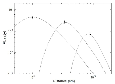
Figure 1: The L-C of three ejecta corresponding to Eq. (2). The three peaks corresponds to three knots at different distances to the core, C1,Ca and C4.

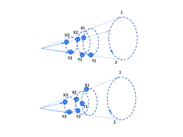
Figure 2: A schematic figure demonstrates knots produced by activities of the cental engine. Knots X1-X3 are produced by one pulse, and Y1-Y3 another. The upper panel corresponds to knots with small discrepancy in precession phases; and the knots of the bottom panel differ significantly in precession phases.

Consequently, during a pulse (not necessarily a constant), a numbers of bursts, say, 10, are generated, and only a few of them can reproduce L-Cs as shown in Fig. 1. Other bursts may produce knots at places deviating significantly from the deceleration radius or with flux density much weaker than that in Fig. 1. Thus, statistically the pattern formed at each pulse is stable, in which the knot-core distance of a knot is approximately constant or constrained in a certain range. A schematic demonstration of such knot production is shown in Fig. 2, in which X1-X3 correspond to knots produced in one pulse, and Y1-Y3 by another pulse. The upper panel differs from the bottom one in precession phase, the former has small discrepancy and the latter one large.

Therefore, at a direction slightly differs from the previous one, once the energy ejection of the pulse and the matter density etc satisfy the parameters of Table 1, knots with L-Cs as shown in Fig. 1 can be reproduced again. The small phase discrepancy among the knots produced in one pulse of the central engine results in the pattern like, knots X1-X3, and large phase discrepancy corresponds to the pattern of Y1-Y3 in Fig. 2.

On longer time scale, e.g., with $10^{3}$ pulses, the change of jet precession phase is of $\sim 10$deg, during which the matter density can be variable through e.g., evacuated bubbles around the sources due to previous activities of the jets. By Eq. (2) such a fluctuation in matter density makes the L-C peak at different distance to the core as shown in Fig. 1, which varies the knot-core separation of knots at different directions. Thus, the ring through X1 and Y1, as shown in Fig. 2, can be tilted, so are rings through X2,Y2 and X3,Y3.

Therefore, the formation of multi-knot morphology can be realized by extending the former non-ballistic model, where several knots are produced along the jet axis. And by the jet precession, these knots cause ring like traces at different separation to the core. Observing at different epochs result in the oscillation of ridge lines.

The ring like pattern corresponds to the knot produced at the deceleration radius. Comparatively, spiral patterns correspond to the knots produced between the deceleration radius and the core, which can be interpreted by the shock-in-jet model.

Thus simply replacing the knot-core distance, $R_{d}$ of Gong(2008), describing the precession of one knot under the non-ballistic model by the multi-knot, $R^{i}$ (where $i=1,2,3...$ corresponds to different knots). The projection of $R_{i}$ to $\Delta\delta$ and $\Delta\alpha$ axes gives,

$$R^{i}_{\alpha} = R^{i}[\sin\lambda\sin\eta^{i}]\sin\xi+R^{i}[\cos\lambda\sin I-\sin\lambda\cos I\cos\eta^{i}]\cos\xi\,,$$

$$R^{i}_{\delta} = R^{i}[\sin\lambda\sin\eta^{i}]\cos\xi-R^{i}[\cos\lambda\sin I-\sin\lambda\cos I\cos\eta^{i}]\sin\xi\,,$$ (3)

where $\lambda$ is the opening angle of the precession cone, $I$ is the inclination angle between the jet rotation axis and LOS. The precession phase is $\eta^{i}=\dot{\Omega}t+\eta^{i}_{0}$ ($\dot{\Omega}$ is the precession velocity of the jet, $\eta_{0}$ is the initial phase of each knot). Projecting $R^{i}$ into the coordinate system $x-y-z$, where the $x$-axis is towards the observer. Then rotating around the $x$-axis for angle $\xi$, so that the new $y$-axis ($\Delta\delta$) will point north, and the new $z$-axis ($\Delta\alpha$) will point east. The position angle of a knot can be simply obtained by

$$\psi=tan^{-1}(\Delta\alpha/\Delta\delta)\,.$$ (4)

3 Application to AGN and X-ray binary

3.1 Oscillation of ridge line

The blazar S5 1803+784 is a flat-spectrum radio source at high declination (Witzel, 1987). Geodetic and astronomical VLBI data gathered at 8.4 and 5 GHz between 1979-1987 showed that the component located at 1.4 mas from the core appears stationary (Schalinski et al., 2003; Witzel, 1988). The stationary component was found to have non-constant core separation or oscillatory type behavior (Britzen et al., 2005). And recently the oscillation of ridge lines of S5 1803+784 is reported (Britzen et al., 2010a).

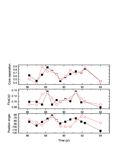
Figure 3: The observed (filled squares corresponding to Britzen et al. 2010) and fitted (opened circles) evolution of core separation (mas), flux and position angle (deg) of one component, C1 of 1803, in the time interval between 1984-1996. The corresponding $\chi^{2}$ from top to bottom panel are 6.3, 0.33, and 90.9 respectively.

In the following we describe the fitting of the kinematics in the pc-scale jet of 1803 by the extended non-ballistic superluminal model of Section 2. The evolution of core separation, flux and position angle of one component, C1, in the time interval between 1984-1996 are observed (Britzen et al., 2010a), as denoted by the filled squares shown in Fig. 3. Under the non-ballistic scenario, the behavior of C1 is simply a conical precession of one knot, projecting to the plane of sky.

With the fitting parameters of Table 1, the peaks of L-Cs in Fig. 1 can account for the observational knots, e.g., C1,Ca and C4 of 1803 (Britzen et al., 2010a). By Fig. 1, at a time scale of half a year, the peaks can decline for 20$\%$-10$\%$. More rapid declination is expected in case of larger spectral index of electron, $p_{0}$, or a radiative dynamics of the shock(Sari et al., 1998). And considering the effect of Doppler boosting, the L-C of a knot can vary more dramatically.

The flux fitting of Fig. 3 corresponds to a bulk speed of $\beta_{b}(R_{i})\sim 0.3-0.6$. Therefore, the core separation, position angle, and flux density of C1, can be fitted by Eq. (2.2), Eq. (4) and Eq. (1) respectively. The variation of separation, position angle and flux of C1 (Britzen et al., 2010a) are fitted by two groups of free parameters. Group A contains 9 global parameters, such as precession speed of jet axis, the opening angle of precession cone and the bulk speed as shown in the first row of Table 2. Group B includes 13 oscillation parameters, denoting the deviation of the distance of component C1 to the core at 13 different epochs from the averaged value as shown in Table 2. These two groups of parameters totally 22, fit three figures, the evolution of the core separation, flux and position angle at 13 epochs, totally $13\times 3=39$ observational points. The three fitting results are reasonable well, as shown in Fig. 3. Notice that in the fitting of position angle and flux of Fig. 3 (26 observational points) only the 9 global parameters are needed, as shown in the first row of Table 2.

Other components, C2,C3…can be treated similarly, except discrepancies on the knot-core separations and phases. The projection of these knots at different time explains the oscillation of ridge lines observed (Britzen et al., 2010a). Variation of knot-core distance up to 50 percent of the average one, $R_{0}$, is needed in the fitting of Fig. 3, which indicates the fluctuation of ISM distribution and hence large discrepancy in knot-core distances at different directions.

The time taken by a knot to precess for tangent distance of the size of a knot, $\delta r$, is $\delta t_{pr}=\delta\eta_{r}/\dot{\Omega}$, where $\delta\eta_{r}=\delta r/(R^{i}\sin\lambda)$. The cooling time of a knot, $\delta t_{co}$, corresponding to, i.e., the time taken for the radio peak to decline for a certain percentage, can be inferred from the L-C, as shown in Fig. 3.

3.2 Precessing jet nozzle

Very Long Baseline Array (VLBA) in an observing mode sensitive to linear polarization at wavelength 7 mm with a resolution of order of 0.2mas has been performed on BL Lac at 17 regular epochs from 1998.23 to 2001.28 (Stirling et al., 2003).

The observations suggest relatively straight trajectories near the core, increasing in curvature at large separations to the core(greater than 1-2 mas). The observed continuation of the trajectory of component S10 did not fit the prediction of helical model (Denn et al., 2000).

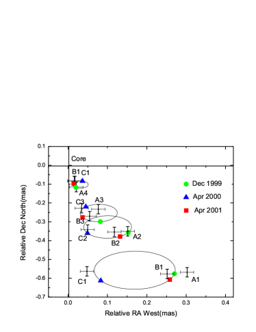
Figure 4: The observed and fitted ridge lines of BL Lac (Stirling et al. 2003). Points with error bars labeled A1-A4, B1-B4 and C1-C4 are observed in December 1999, April 2000 and April 2001, respectively. The ellipses are predicted by the non-radial model.

As shown in Fig. 4, ridge lines formed by four knots are observed in December 1999, April 2000 and April 2001 (Stirling et al., 2003), which are labeled by points with error bars, A1-A4, B1-B4 and C1-C4 respectively.

The largest discrepancy appears in the ridge line in December 1999, when the helical model predicts a ridge line approximately along the vertical line from (0.0, 0.0) to (0.0, -0.6), the observed ridge line corresponds to points with error bars, A1-A4 in Fig. 4.

By the non-ballistic model, with fitting parameters of Table 3, the observed knots, the ridge lines A1-A4, B1-B4, and C1-C4, can be well fitted by the filled circles, squares and triangles respectively, as shown in Fig. 4. The relatively small discrepancies in a few points in Fig. 4 can be improved by assuming small variation in the core-knot separation. This means that even the straight ridge lines can be explained by knots predicted by the non-ballistic scenario. Consequently, the true ballistic jet motion should occur in the region even closer to the core than these straight ridge lines of Fig. 4.

It was suggested that initial straight component trajectories and the subsequent bending jet is due to a transition from a ballistic fashion to non-ballistic flow (Stirling et al., 2003).

Whereas, from the point of view of non-ballistic model, the non-radial knot can be interpreted simply by extending the fitting of Fig. 4 to knots with larger separation to the core and with larger discrepancy in the initial precession of each knot, which is further discussed in Section 4.

3.3 Two puzzling knots of SS 433

Interestingly, the non-radial motion displayed in AGNs is also observed in the famous X-ray binary system of SS 433. , in which anti-parallel jets traveling near-relativistically are detected in observations across X-ray, optical and radio wavelengths (Margon, 1984). The strong and broad emission lines have been identified as redshifted/blueshifted emission from collimated jets with intrinsic velocity of $\simeq 0.26c$ (Abell& Margon, 1979). The periodic change of Doppler shift of emission lines with time is widely accepted to be a precessing ballistic jet with a period of 164d.

Although the jet motion of SS 433 is less than the speed of light, the behavior of which is strikingly similar to the superluminal sources. In the 2001 observation of arcsec-scale X-ray jets of SS 433 (Migliari et al., 2005). As shown in the top panel of Fig. 5, a knot became brighter from May 8 to May 10 (knot A) and subsequently on May 12 it appeared to be moving along a precession trace to a new place (knot B).

The observation of the two knots seems simple, it is not easy to understand in the context of the standard ballistic plus precession model either. If knots A and B are results of one ball traveling from A to B, then its position angle should not change so dramatically, and the discrepancy in the travel time of these two knots to the observer should be much longer than the reported 2 d. On the other hand, if knots A and B are caused by two ejections, then B should be ejected earlier than A. As a result, B should appear earlier than A. This is contrary to the observation. Moreover, the ballistic scenario predicts that both knots A and B should move outwardly as a whole. Whereas, one cannot find such a motion either.

To explain the motion of these two knots under the standard ballistic model, the underlying faster outflow scenario is proposed, in which the two knots ejected from the binary core first, and later a fast shock wave propagates from the core through the jet and hits first the knot A and then knot B (Migliari et al., 2005). This requires the central engine to switch on different modes of power at different time.

In some cases the jet motion like knots A and B of SS433, have been used as evidences contradicting to the scenario of jet precession. In fact, the problem is originated from the ballistic assumption rather than the jet precession. Therefore, the relationship between non-radial and radial jet motion needs to be discussed.

The model of two knots moving at certain position and then brightened up by two shocks sequently (Migliari et al., 2005), is shown in the middle panel of Fig. 5. Knot B is at a distance of $1.7\times 10^{17}$cm from the core, which was ejected from the binary system about 40d earlier than knot A, and is moving towards us with an angle to LOS of $\sim 80$deg. The shock wave interact first with knot A and then with knot B. When the shock interacts with knot A, the distance between A and B is about 20 light days. Therefore, the shock wave has to travel the projected distance between the two knots in about 22d. In order to observe the brightening of the two components within two days, the shock has to travel with a velocity of $v\sim 0.5$c.

The non-ballistic model provides a simpler scenario, in which knot A with a X-ray peak count of 75.2 at $\sim 10^{17}$cm (Migliari et al., 2005) can be reproduced at the deceleration radius $r_{\rm d}$ (measured from the central), where the swept-up medium by the jet has an energy comparable to that of the outflow (Blandford & Mckee, 1976),

$$r_{\rm d}=(\frac{3E}{4\pi\gamma_{0}^{2}nm_{p}c^{2}})^{\frac{1}{3}},$$ (5)

where $\gamma_{0}$ is the initial Lorentz factor of the outflow. So the separation of knot A to the core of $\sim 10^{17}$cm corresponds to $E_{51}^{\frac{1}{3}}\gamma_{0,5}^{-\frac{2}{3}}n_{0}^{\frac{1}{3}}\sim 0.54$, where $E_{51}$ is $E$ in units of $10^{51}$ erg, $\gamma_{0,5}$ is $\gamma_{0}$ in units of 5, $n_{0}$ is in units of 1 ${\rm cm}^{-3}$.

By the non-ballistic model, knots A and B observed in SS 433 can be fitted by the precession trace as shown in the bottom panel of Fig. 5. The fitting parameters are given in Table 2. Therefore, knots A and B can be lying on the precession trace given by Eq. (2.2). The deviation in precession phase of A and B corresponding to a time discrepancy of 38 days. It takes 36 days for a signal to propagate from A to B. Hence knot B is brightened up two days later than knot A, which satisfies the observation (Migliari et al., 2005) in a much simpler way.

The fitting of the two dimension trajectory of knot A and B by Eq. (2.2) actually needs 4 equations (corresponding to the coordinate of A and B), and the 2d deviation in propagation time imposes another constraint on the discrepancy of the knot-observer distance. Therefore, the bottom panel of Fig. 5 can be recognized as obtaining the five variables, as shown in Table 4 by five equations (constraints).

Note that in principle, no matter how many input parameters are used, the trajectory of knot A and B cannot be fitted by the ballistic plus precession scenario directly.

4 The nature of bent jet

The origins of jet curvature in the one-knot case has been discussed in Gong (2008). Here it is extended to the multi-knot case, and the association of the two types of bent jets is addressed.

Within the non-ballistic model, there are two origins of jet curvature. The first one is caused by the knots moving at different rings. In this case, the phase discrepancies between two neighboring knots at different separations are given, $\delta\eta^{i}=\dot{\Omega}\delta t^{i}+\eta^{0}$, in which $\delta t^{i}$ can be written,

$$\delta t^{i}\equiv t^{i+1}-t^{i}=\delta R^{i}/v^{i+1}+[x^{i+1}-x^{i}]/c\,,$$ (6)

where $x^{i}$ is the knot-observer distance of knot $i$, $\delta R^{i}\equiv R^{i+1}-R^{i}$ is discrepancy of the core-knot distance between knots $i$ and $i+1$, and $v^{i+1}$ is the bulk speed of knot $i+1$. A dramatic reduction of bulk velocity between e.g., knot 2 and 3, $v^{3}<<v^{2}$, results in $\delta R^{2}/v^{3}\gg\delta R^{2}/v^{2}$, which leads to a large phase discrepancy, $\delta\eta^{2}$ between knot 2 and 3. In such case, the jet is bent sharply at knot 2 by Eq. (6) and Eq. (2.2). This explains the wiggling structure of 0548+165 (Mantovani et al., 1998), and the two rectangular pattern in BL Lac object PKS 0735+178 (Britzen et al., 2010b).

Knots produced in the case of small phase discrepancy and large phase discrepancy can be demonstrated by the upper and bottom pattern of Fig. 2 respectively, which explains the variation of ridge lines of BL Lac (Stirling et al., 2003) and the oscillation of ridge lines of 0735+178 and 1803 respectively.

The second origin of jet curvature corresponds to the trajectory produced by a singular knot, with negligible variation in radial separation, which is simply part of an ellipse in the plane of the sky, which has been discussed (Gong, 2008).

From the stand of Eq. (6), the curvature in such one-knot case can be obtained simply by removing the first term at the right hand side of Eq. (6), which well explains the curvature of knots A and B in SS 433.

In fact, such a singular knot curvature determined by Eq. (6) and Eq. (2.2) can explain the non-radial behavior revealed in other AGN sources, where outflow are aligned with the local jet direction, suggesting the jet flow occurs along preexisting bent channels, like 0738+313 and quasar NRAO 150 (Kellermann et al., 2004; Lister et al., 2009; Agudo et al., 2007).

By the time derivatives of Eq. (2.2), $\ddot{R}^{i}_{\alpha}$ and $\ddot{R}^{i}_{\delta}$ can be obtained, which naturally provides the acceleration perpendicular to the velocity vector displayed in AGN components (Lister et al., 2009).

5 Why 98.5$\%$ outward motion

Although the problem that the jet features showing an overwhelming tendency of outward motion away from the core has been addressed (Gong, 2008), it can be further discussed in three aspects.

The first is that most jets of AGNs and X-binaries are observed at the stage before ejectors reaching the deceleration radius, which is dominated by the ballistic scenario.

The second is that some sources have a small opening angle of precession cone, the geometry of which displays the oscillation of ridge line like BL Lac (Stirling et al., 2003). In such case, outward and inward motions are performed in limited region, and motion perpendicular to the ridge line is obvious, which is usually cataloged to the helical motion instead of inward motion.

The third one is for those sources that the jet axis really through LOS during the precession of jet. In such case, following mechanism can make asymmetry in the inward and outward motion of such a precession jet.

By Eq. (6), a mildly curved jet appears when $\delta R^{i}/v^{i+1}$ is not too large at different locations of the jet. As shown in Fig. 6, a knot is produced at the deceleration radius at a precessing and curved jet. Since the knot actually corresponds to a region, e.g., the knot C1 of 1803 is about $\delta r\approx 0.5$ mas(3pc) in diameter (Britzen et al., 2010a). Owing to the energy dissipation at the deceleration radius, the bulk speed of ejector reduces to typically half of its original speed, which can be simplified as composed of several sub-knots, each corresponds to a sub-jet as $a$ and $b$ in the left panel of Fig. 6. According to the standard GRB model, a dramatic reduction of bulk speed occurs at the deceleration where the knot produced (e.g., from $\gamma=10$ to $\gamma=2$), so that the upstream sub-knots posses larger bulk speed than those of the downstream ones, $\gamma_{i}>\gamma_{i+1}$, by a factor of a few. Hence through $\theta_{i}=1/\gamma_{i}$, the half opening angle of emission beam of these two sub-knots, $i$ and $i+1$, satisfy, $\theta_{i}<\theta_{i+1}$. Thus the effective emission beam of the knot is extended, with higher brightness at upstream region and lower at the downstream region, as shown in the middle of Fig. 6.

With $\alpha$ represents the misalignment angle between two sub-jets $a$ and $b$ corresponding to the two knots having the minimum and maximum beam opening angles, $\theta_{min}$ and $\theta_{max}$. E.g., for knot C1 of 1803, $\alpha\approx\delta r/R_{0}=0.5/0.8=0.6$rad. As shown in the left panel of Fig. 6, a knot beam extended significantly when $\alpha\gg\theta_{min}$(e.g.,$\theta_{min}\approx 0.1$, with $\gamma\approx 10$); and a negligible extension occurs when $\alpha\approx\theta_{min}$ (e.g.,$\theta_{min}\approx 0.5$, with $\gamma\approx 2$).

The precession of the curved jet of the left panel of Fig. 6, is equivalent to a fix jet and a change of the observer’s LOS, as shown in the middle of Fig. 6. At epoch 1, the observer sees a brief inward motion, and epochs 2-4 correspond to the long outward motion due to the extended emission beam, as shown in right panel of Fig. 6. Thus the very large numbers of observed outward motions as opposed the inward ones results when most of the knot emission beams are deformed considerably. Consequently this causes serious asymmetry at two sides of the line connecting the observer, the knot and the core (case 2 in the middle and right hand side of Fig. 6).

Notice that according to this scenario, the size of an inwardly moving knot is not necessarily large than that of an outward one. Whereas, the explanation of inward motion by jet bending back and across LOS (Marscher et al., 1991) predicts larger size of inward knot than that of outward ones, considering the lateral expansion of a knot at very longer distance from the core.

In this paper, multi-knot corresponds to a series of knots produced by jet-matter interaction. Singular knot is an individual knot produced by the jet-matter interaction. And sub-knot represents a singular knot (or one of the multiple knots) at different stage of evolution near the deceleration radius.

6 Discussion and conclusion

This paper shows that generally the interaction of jet and ambient matter can reproduce a number of knots along the jet, both at the region near the deceleration radius and at the region between the deceleration radius and the core. Knots produced at the region near the deceleration radius are simulated by the dynamics of jet-matter interaction. And the motion of such multi-knot is used to explain the changes of ridge line such as BL Lac (Stirling et al., 2003) and 1803 (Britzen et al., 2010a). On the other hand, knots produced between the deceleration radius and the core can be understood in the context of the Shock-in-jet model (Marscher & Gear, 1985), in which a spiral pattern is expected when the jet precesses. In other words, this paper not only extends the former non-ballistic model from one-knot to multi-knot, but also discusses the relationship between the non-ballistic model and the Shock-in-jet model.

Interestingly, jets observed by the early long base line technique e.g., in 1970s-1980s, appear more straight than those observed in the past ten years with much improved sensitivity. From the view of non-ballistic model, this is expected. Because even a curved jet can behave as a straight one, due to the low sensitivity observation favors to observe bright knots having small misalignment between the jet axis and LOS, which is Doppler boosted strongly. In other words, it is this selection effect that makes the early jets appear straight. By the improved sensitivity, weaker and weaker part of jet is measurable, so that more and more curved jet appear. Thus, the ratio of non-radial over radial motion of jet should increase with time.

7 Acknowledgments

We thank S. Britzen, A. Witzel, and J.A. Zensus for helpful discussions and suggestions in the manuscript. We also thank Z.Q. Shen for useful comments of the manuscript. This research is supported by the National Natural Science Foundation of China, under grand NSFC11178011. And 11033002, by the National Basic Research Program of China (973 Program, Grant No. 2009CB824800).

Table 1: The fitting parameters of three knots by the standard afterglow of GRB model.

knot	$\Gamma_{0}$	$\varepsilon_{e}$	$\varepsilon_{B}$	$\theta_{j}$	$E_{0}$	$n_{0}$	$p_{0}$
1	5.0	0.1	0.01	0.01	$6.0\times 10^{59}$	0.2	2.1
2	5.0	0.1	0.01	0.02	$2.0\times 10^{59}$	0.02	2.3
3	5.0	0.1	0.01	0.03	$8.0\times 10^{58}$	0.002	2.8

The initial isotropic equivalent kinetic energy of the outflow, $E_{0}$ (erg), opening angle of jet, $\theta_{j}$ (rad), initial Lorentz factor,$\Gamma_{0}$, density of ambient matter,$n$, spectral index of electron, $p_{0}$, the fraction of total shock energy acquired by the shocked electron and magnetic field, $\varepsilon_{e}$ and $\varepsilon_{B}$ respectively.

Table 2: The fitting parameters of the knot-core separation, position angle and flux density of component C1 of 1803 as shown in Fig. 6.

$\xi$	$\dot{\Omega}$	$I$	$\lambda$	$\eta_{0}$	$R_{0}$	$\beta_{b}$	$n$	$S_{0}$
1.43	36.3	1.27	0.28	4.24	0.82	0.34	2.00	0.10
$\delta R_{1}$	$\delta R_{2}$	$\delta R_{3}$	$\delta R_{4}$	$\delta R_{5}$	$\delta R_{6}$	$\delta R_{7}$	$\delta R_{8}$	$\delta R_{9}$
-0.37	-0.45	0.12	0.17	-0.018	-0.16	-0.31	-0.20	-0.05
$\delta R_{10}$	$\delta R_{11}$	$\delta R_{12}$	$\delta R_{13}$
0.00	-0.046	0.060	-0.37

The average knot-core separation, $R_{0}$, and the deviation of the knot-core distance from the average value at different time, $\delta R_{i}$ ($i=1-13$), are in unite of mas; $\dot{\Omega}$ is in deg/yr, $\xi$, $\lambda$, $I$ and $\eta_{0}$ are in rad. The two parameters, $n$ and $S_{0}$ denote the index $3-\alpha$ and the flux density at the righthand side of Eq. (1) respectively.

Table 3: The fitting parameters of BL Lac (Stirling et al. 2003).

$\xi$	$\eta^{\ast}$	$I$	$\lambda$	$R$	$\Omega$
73.1	$30.0^{\ast}$	11.6	2.0	0.54	0.67

The core-knot separation ($R$) is in mas, the precession velocity, $\Omega$ is in deg/d, and all other parameters are in degree. ^∗ 30.0 deg corresponds to the initial phase of the smallest ellipse in Fig 5, other initial phases from from to large are, 0.0deg, 20.0deg and 15.0 deg respectively.

Table 4: The parameters derived from the fitting of the trace of knots A and B.

$\xi$	$\eta$	$I$	$\lambda$	$R$
1.0	60.0	72.5	30.7	2.0

The core-knot separation ($R$) is in arcsec, and all other parameters are in degree.

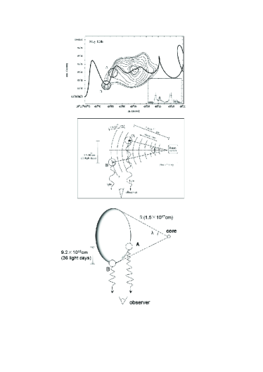
Figure 5: The observation and interpretation of knots A and B of SS433. Top panel is the zeroth-order HETGS image taken on 2001 May 12. Middle panel is the sketch of the orientation of the east jet of SS 433, which interprets the observations of knots A and B in context of the slowly moving clouds energized erratically by a more powerful, faster, unseen flow. The top and middle panels are adopted from Migliari et al. (2005). The bottom panel is the sketch explaining the observations of knots A and B by the non-ballistic model.

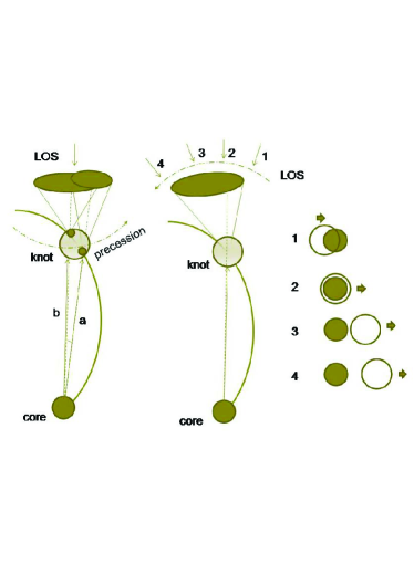
Figure 6: A schematic explanation of the very large numbers of observed outward motions as opposed the inward ones. The curved jet precesses along the dash-dotted direction, and the observed knot can be seen as composed of several sub-knots, as shown in the left panel. The precession of the curved jet of the left panel is equivalent to a fix jet and a motion of the observer’s LOS as shown in the middle panel. The right panel gives the observed knot, hollowed circle, and the core, filled circle.

References

- Abell& Margon (1979) Abell, G.O. & Margon, B., 1979, Nat., 279, 701
- Agudo et al. (2007) Agudo, I. et al., 2007, A&A, 476, L17
- Blandford & Mckee (1976) Blandford, R. D. & McKee, C. F., 1976, Physics of Fluids, 19, 1130
- Britzen et al. (2005) Britzen S., Kam, V. A., Witzel, A., Agudo, I., Aller, M. F., Aller, H. D., Karouzos, M., Eckart, A., & Zensus, J. A., 2009, A&A 508, 1205
- Britzen et al. (2009) Britzen S., Witzel, A., & Krichbaum, T.P. et al., 2005, MNRAS 362, 966
- Britzen et al. (2010a) Britzen, S., Kudryavtseva, N. A., Witzel, A., Campbell, R. M., Ros, E., Karouzos, M., Mehta, A., Aller, M. F., Aller, H. D., Beckert, T.,& Zensus, J. A., 2010a, A&A, 511, 57
- Britzen et al. (2010b) Britzen, S., Witzel, A., Gong, B. P., Zhang, J. W., Krishna, G., Goyal, A., Aller, M. F., Aller, H. D., & Zensus, J. A., 2010b, A&A, 515, 105
- Denn et al. (2000) Denn ,Grant R., Mutel, Robert L., & Marscher, Alan P., 2000, ApJS, 129, 61
- Gliozzi et al. (2004) Gliozzi, M., Sambruna, R. M., Brandt, W. N., Mushotzky, R.,& Eracleous, M., 2004, A&A, 413, 139
- Gong (2008) Gong, B.P., 2008, MNRAS, 389,315
- Homan et al. (2009) Homan, D. C., Kadler, M., Kellermann, K. I., Kovalev,Y. Y., Lister, M. L., Ros, E., Savolainen,T., & Zensus, J. A., 2009, ApJ, 706, 1253
- Huang et al. (2000) Huang, Y. F., Gou, L. J., Dai, Z. G.,& Lu, T., 2000, ApJ, 543, 90
- Hummel et al. (1992) Hummel, C. A., Schalinski, C. J., Krichbaum, T. P., Rioja, M. J., Quirrenbach, A., Witzel, A., Muxlow, T. W. B., Johnston, K. J., Matveenko, L. I. & Shevchenko, A., 1992, A & A, 257, 489
- Kellermann et al. (2004) Kellermann, K. I., Lister M. L., Homan D. C., Vermeulen R. C., Cohen M. H., Ros E., Kadler M., Zensus J. A., & Kovalev Y. Y., 2004, ApJ, 609, 539
- Lister et al. (2009) Lister, M. L., Cohen,M. H., Homan,D. C., Kadler, M., Kellermann, K. I., Kovalev,Y. Y., Ros,E., Savolainen, T., & Zensus, J. A., 2009, AJ, 138, 1874
- Mantovani et al. (1998) Mantovani F. et al., 1998, A&A, 332, 10
- Margon (1984) Margon, B., 1984, Ann. Rev. Astron. Astrophys, 22, 507
- Marscher & Gear (1985) Marscher, A. P. & Gear, W. K., 1985, ApJ, 298, 114
- Marscher et al. (1991) Marscher,A.P., Zhang, Y. F., Shaffer, D. B., Aller,H. D.,& Aller, M. F., 1991, ApJ, 371, 491
- Migliari et al. (2005) Migliari, S., Fender, R. P., Blundell, K. M., M ndez, M.,& van der Klis, M., 2005, MNRAS, 358, 860
- Rani et al. (2010) Rani B. et al., 2010, ApJ, 719, L153
- Rees (1966) Rees, M. J., 1966, Nat, 211, 468
- Sari et al. (1998) Sari R., Piran, T., & Narayan, R., 1998, ApJ, 497, L17
- Spada et al. (2001) Spada, M. et al. 2001, MNRAS, 325, 1559.
- Stirling et al. (2003) Stirling,A. M., Cawthorne, T.V., Stevens, J. A., Jorstad, S. G., Marscher, A. P., Lister, M. L., G mez, J. L., Smith, P. S., Agudo, I., Gabuzda, D. C., Robson, E. I. & Gear, W. K., 2003, MNRAS, 341, 405
- Schalinski et al. (2003) Schalinski, C.J. et al., 1988, In: M.J. Reid, J.M. Moran (eds.), Proc.IAU Symp. 129, Kluwer, Dordrecht, 359
- Wang et al. (2003) Wang, X. Y., Dai, Z. G., & Lu, T., 2003, ApJ, 592, 347
- Witzel (1987) Witzel A., 1987, In: J.A. Zensus, T.J. Pearson (eds.), Superluminal Radio Sources, Cambridge University Press, Cambridge, 83
- Witzel (1988) Witzel A., et al. 1988, A&A, 206, 245