Charged colloids in an aqueous mixture with a salt

Abstract

We calculate the ion and composition distributions around colloid particles in an aqueous mixture, accounting for preferential adsorption, electrostatic interaction, selective solvation among ions and polar molecules, and composition-dependent ionization. On the colloid surface, we predict a precipitation transition induced by strong preference of hydrophilic ions to water and a prewetting transition between weak and strong adsorption and ionization. These transition lines extend far from the solvent coexistence curve in the plane of the interaction parameter $\chi$ (or the temperature) and the average solvent composition. The colloid interaction is drastically altered by these phase transitions on the surface. In particular, the interaction is much amplified upon bridging of wetting layers formed above the precipitation line. Such wetting layers can either completely or partially cover the colloid surface depending on the average solvent composition.

I introduction

Extensive efforts have been made to understand the interaction among ionized colloid particles in a solvent Dej ; Ov ; Russel ; Ohshima ; LevinReview , because they form model crystal and glass at high densities. Recently, considerable attention has also been paid to the effect of preferential adsorption of one of the components in a mixture solvent. Several groups Beysens ; Maher ; Kaler ; Guo ; Bonn observed aggregation of colloidal particles near the coexistence curve in one-phase states of a binary mixture of 2,6-lutidine and water. For small ionization the adsorption of lutidine was increased in water-rich states, while for large ionization that of water was increased in lutidine-rich states. This means that the colloid surface can either repel or attract water, depending on the degree of ionization. It is worth noting that polyelectrolytes are often hydrophobic without ionization, but becomes effectively hydrophilic even at low ionization Barrat ; Holm ; Rubinstein .

At high colloid concentrations, a flocculated phase rich in colloids emerges Beysens , which changes from gas, liquid, fcc crystal, and glass with increasing the colloid concentration Guo . Such aggregation was claimed to be a result of a true phase separation in ternary mixtures Kaler . A microscopic theory by Hopkins et al. Evans indicated the aggregation mechanism. They treated neutral colloids coated by a thick adsorption layer rich in the preferred component in one-phase environments rich in the other component. They found that this adsorption is intensified near the coexistence curve, strongly influencing the colloid interaction.

In understanding these experiments, however, attention has not been paid to the selective solvation (hydration for aqueous mixtures) among charged particles (ions and ionized parts on the colloid surface) and polar solvent molecules Is . The solvation effects have not yet been adequately investigated in soft materials, but they can influence the phase separation behavior profoundly and even give rise to a new phase transition Onuki-Kitamura ; OnukiPRE ; Nara ; Current . The solvation chemical potential $\mu_{\rm sol}(\phi)$ of a hydrophilic ion stems from the ion-dipole interaction and strongly depends on the ambient composition of water. In electrochemistry, the following chemical potential difference has been measured Hung ; Osakai :

$$\Delta\mu_{\rm sol}^{\alpha\beta}=\mu_{\rm sol}(\phi_{\beta})-\mu_{\rm sol}(\phi_{\alpha}),$$ (1.1)

between two coexisting phases, where $\phi_{\alpha}$ and $\phi_{\beta}$ are the bulk water compositions in the two phases. This quantity is the so-called Gibbs transfer free energy per ion, which determines the ion partition and a Galvani potential difference between the two phases. Its magnitude typically much exceeds $k_{B}T$ (about $15k_{B}T$ for Na⁺ and Cl^- in water-nitrobenzene at room temperatures). Furthermore, the dissociation of ionizable groups on the colloid surface should be treated as a chemical reaction sensitively depending on the local environment (the solvent composition and the local electric potential) as in the case of polyelectrolytes Barrat ; Holm ; Bu2 ; Onuki-Okamoto . Therefore, even very small composition variations around the colloid surface can induce significant changes in the ion distribution, the electric potential, and the degree of ionization, so it can drastically alter the colloid interaction.

Historically, the colloid interaction has been supposed to consist of the screened Coulomb repulsive infraction $F_{\rm DLVO}$ and the van der Waals attractive interaction $F_{\rm vdw}$ since the celebrated theory developed by Derjaguin, Landau, Verway, and Overbeek (DLVO) Russel ; LevinReview ; Dej ; Ov . For two colloid particles with radius $a$, the former reads

$$F_{\rm DLVO}=\frac{{\bar{Q}}^{2}e^{-\kappa(d-2a)}}{\bar{\varepsilon}(1+\kappa a)^{2}d}$$ (1.2)

where $d$ is the distance between two colloid centers, $\bar{Q}$ is the average charge on a colloid particle, $\bar{\epsilon}$ is the average dielectric constant (at the average composition for a mixture solvent), and $\kappa$ is the Debye wave number. The latter arises from the pairwise van der Waals interaction ($\propto-1/r^{6}$) among constituent molecules, where $r$ is the distance between two molecules. In terms of the Hamaker constant $A_{\rm H}$, $F_{\rm vdw}$ between two identical colloids with radius $a$ is written as Russel

$$F_{\rm vdw}=-\frac{A_{H}}{6}\bigg{[}\frac{2a^{2}}{d^{2}-4a^{2}}+\frac{2a^{2}}{d^{2}}+\ln\bigg{(}1-\frac{4a^{2}}{d^{2}}\bigg{)}\bigg{]}.$$ (1.3)

It grows for short separation $\ell=d-2a\ll a$ as

$$F_{\rm vdw}\cong-{A_{\rm H}}a/{12}{\ell},$$ (1.4)

while it decays as $-{16A_{\rm H}}a^{6}/{9}{d^{6}}$ for long separation $\ell\gg a$. We assume that $F_{\rm vdw}(d)$ should saturate at a short distance on the order of the solvent molecular diameter $a_{0}$ ($\sim 3{\rm\AA}$). Then $F_{\rm vdw}(d)$ decreases down to $-A_{H}a/12a_{0}$ at contact. The size of $A_{H}$ strongly depends on binary mixtures and colloid particles under investigation and can be made small by matching the dielectric constants of the colloid and the solvent. In this paper, $F_{\rm vdw}$ will not be included in our theoretical scheme for simplicity.

In binary mixtures, the adsorption-induced composition disturbances give rise to an attractive interaction $F_{\rm ad}$ between two colloid particles Beysens . A linear theory can then be developed when the adsorption and the ionization are both weak. Further in the special case of weak selective solvation, the pair interaction is the sum of $F_{\rm DLVO}$ in Eq.(1.2) and $F_{\rm ad}$ given by

$$F_{\rm ad}=-A_{\rm ad}a^{4}\xi^{2}\frac{e^{-\ell/{\xi}}}{(a+{\xi})^{2}d},$$ (1.5)

where $\xi$ is the correlation length growing near the solvent criticality. The coefficient $A_{\rm ad}$ is proportional to $h_{1}^{2}$, where $h_{1}$ is the surface field arising from preferential molecular interactions between the surface and the two solvent species Cahn ; Binderreview ; Bonnreview . In deriving Eq.(1.5), $h_{1}$ is assumed to be small and Eq.(1.5) is invalid very close to the criticality h1 ; nevertheless, $F_{\rm ad}$ becomes the dominant interaction at long distances for $\xi>\kappa^{-1}$. We shall see that $F_{\rm ad}$ can exceed $F_{\rm vdw}$ even at the molecular separation $a_{0}$ for small $A_{H}$. Furthermore, on approaching the solvent criticality without ions, the adsorption-induced interaction among solid objects (plates, rods, and spheres) becomes universal (independent of the material parameters) in the limit of strong adsorption Fisher , so it has been called the critical Casimir interaction Krech ; JSP ; Nature2008 ; Gambassi . However, it should be affected by ions for strong selective solvation.

In this paper, we aim to investigate the ion effects on the colloid interaction in binary mixtures using a coarse-grained approach. A merit of our approach is that we can treat the preferential solvation in its strong coupling limit. In our recent work Current ; Okamoto , we found that a strongly selective solute can induce formation of domains rich in the preferred component even far from the solvent coexistence curve. We shall see that this precipitation phenomenon can occur on the colloid surface, leading to a wetting layer coating the colloid surface. As another prediction, there can be a first-order prewetting surface transition between weak and strong adsorption far from the solvent criticality, as discussed in our paper on charged rods Onuki-Okamoto . These two phase transitions occur when the volume fraction of the selected component is relatively small ($\phi<\phi_{c}$). With intensified mutual interactions, colloid particles should trigger a macroscopic phase separation to form a floccuated phase Beysens ; Guo ; Kaler . As a closely related example, precipitation of DNA has been observed with addition of ethanol in water B1 ; B2 ; B3 , where the ethanol added is excluded from condensed DNA.

In addition to usual hydrophilic ions, we are also interested in the colloid interaction in the presence of antagonistic ion pairs in aqueous mixtures, where the cations are hydrophilic and the anions are hydrophobic, or vice versa Nara ; Current . A well-known example in electrochemistry is a pair of Na^- and tetraphenylborate BPh${}_{4}^{-}$, where the latter anion consists of four phenyl rings bonded to an ionized boron and acquires strong hydrophobicity. Such ion pairs behave antagonistically in the presence of composition heterogeneities, giving rise to formation of mesophases, as recently observed by Sadakane et al. by adding a small amount of NaBPh₄ to D₂O and tri-methylpyridine Sadakane . They should produce an oscillatory interaction between walls or colloid particles as in the case of liquid crystals Uchida .

The organization of this paper is as follows. In Sec.II, we will present a Ginzburg-Landau model of a binary mixture containing ions and ionizable colloid particles, where the bulk part includes the electrostatic and solvation interactions and the surface part the dissociation free energy. In Sec.III, we will examine the linearized version of our theory for the electrostatic and composition fluctuations as a generalization of the Debye-H$\ddot{\rm u}$ckel and DLVO theories. In Sec.IV, we will discuss how a wetting layer is formed on the colloid surface, which takes place as a precipitation phase transition. In Sec.V, we will present numerical results on the basis of our nonlinear scheme, where we shall encounter precipitation and prewetting phase transitions on the surface even far from the solvent coexistence curve. We shall also see bridging of wetting layers and a changeover between complete and partial wetting.

II Ginzburg-Landau model for a mixture solvent

We suppose monovalent hydrophilic cations and anions in a binary solvent composed of a water-like polar component (called water) and a less polar component (called oil) in a cell with a volume $V$ Onuki-Kitamura ; OnukiPRE ; Okamoto . We also place one or two negatively ionizable colloid particles in the cell. Experimentally, we suppose a dilute suspension of colloid particles in a mixture solvent. To apply our results to such systems, we should set $V=1/n_{\rm col}$, where $n_{\rm col}$ is the colloid density.

For simplicity, we neglect the van der Waals interaction $F_{\rm vdw}$. The Boltzmann constant $k_{B}$ will be set equal to unity in the following.

II.1 Free energy including electrostatics, solvation, and surface interaction

We assume that the counterions coming from the colloid surface are of the same species as the cations added as a salt. The cation and anion number densities are written as $n_{1}$ and $n_{2}$, respectively, while the water composition is written as $\phi$. We treat these variables as smooth functions in space. The total free energy $F_{\rm tot}=F+F_{s}$ consists of the bulk part $F$ and the surface part $F_{s}$. The former is written as

$$F=\int^{\prime}d{\mbox{\boldmath$r$}}[f_{\rm tot}+\frac{TC}{2}|\nabla\phi|^{2}]+\int d{\mbox{\boldmath$r$}}\frac{\varepsilon{\mbox{\boldmath$E$}}^{2}}{8\pi},$$ (2.1)

where $\int^{\prime}d{\mbox{\boldmath$r$}}$ is the space integral in the colloid exterior in the cell and $\int d{\mbox{\boldmath$r$}}$ is that in the whole cell including the colloid interior. The electric potential $\Phi$ is defined even in the colloid interior. We assume that inhomogeneity of $\phi$ gives rise to the gradient free energy, where the coefficient $C$ is a positive constant.

In the first term of Eq.(2.1), the free energy density $f_{\rm tot}$ is the chemical part depending on $\phi$, $n_{1}$, and $n_{2}$ as

$${f_{\rm tot}}=f(\phi)+T\sum_{i}n_{i}\bigg{[}\ln(n_{i}\lambda_{i}^{3})-1-g_{i}\phi\bigg{]}.$$ (2.2)

In this paper, the molecular volumes of the two solvent components take a common value $v_{0}$, though they are often very different in real binary mixtures. As a molecular length, we introduce

$$a_{0}=v_{0}^{1/3},$$ (2.3)

which is supposed to be of order $3{\rm\AA}$. Then $C\sim a_{0}^{-1}$ comment-gra . The colloid radius $a$ is much larger than $a_{0}$. (In our previous papers Onuki-Kitamura ; OnukiPRE ; Nara ; Current ; Okamoto , $a$ has been used to denote the molecular length $v_{0}^{1/3}$.) We neglect the volume fractions of the ions assuming their small sizes. In our numerical analysis, we adopt the Bragg-Williams form Onukibook ,

$$\frac{v_{0}}{T}f=\phi\ln\phi+(1-\phi)\ln(1-\phi)+\chi\phi(1-\phi),$$ (2.4)

where $\chi=\chi(T)$ is the interaction parameter depending on $T$. The critical value of $\chi$ is 2 without ions. In the ionic part of Eq.(2.2), $\lambda_{i}=\hbar(2\pi/m_{i}T)^{1/2}$ is the thermal de Broglie wavelength of the species $i$ with $m_{i}$ being its mass. The dimensionless parameters $g_{1}$ and $g_{2}$ represent the degree of selective solvation Onuki-Kitamura ; OnukiPRE , in terms of which the solvation chemical potential is $\mu_{\rm sol}^{i}={\rm const.}-Tg_{i}\phi$ and the Gibbs transfer free energy is $Tg_{i}(\phi_{\alpha}-\phi_{\beta})$ for the ion species $i$ (see Eq.(1.1)). If $\phi$ is the water composition, we have $g_{i}>0$ for hydrophilic ions and $g_{i}<0$ for hydrophobic ions. In many aqueous mixtures, the amplitude $|g_{i}|$ well exceeds $10$ both for hydrophilic ions and hydrophobic solutes Current .

The last term in Eq.(2.1) is the electrostatic partTojo , where ${\mbox{\boldmath$E$}}=-\nabla\Phi$ is the electric field. The electric potential $\Phi$ is defined in the whole region including the colloid interior. We assume continuity of $U$ through the colloid surface neglecting surface molecular polarization. It follows the Poisson equation,

$$\nabla\cdot{\mbox{\boldmath$D$}}=-\nabla\cdot\varepsilon\nabla\Phi=4\pi\rho,$$ (2.5)

where ${\mbox{\boldmath$D$}}=\varepsilon{\mbox{\boldmath$E$}}$ is the electric flux density. The dielectric constant $\varepsilon(\phi)$ is assumed to be a linear function of $\phi$ in the solvent. Thus it behaves as

$$\varepsilon(\phi) = \varepsilon_{0}+\varepsilon_{1}\phi~{}\quad({\rm colloid~{}exterior})$$ (2.6)

$$= \varepsilon_{\rm p}\qquad\qquad({\rm colloid~{}interior}),$$

which is $\varepsilon_{0}$ in oil (at $\phi=0$), $\varepsilon_{0}+\varepsilon_{1}$ in water (at $\phi=1$), and $\varepsilon_{\rm p}$ in the colloid interior. Let all the charges be monovalent. Then the charge density $\rho$ is written as

$$\rho=e(n_{1}-n_{2})-e\sigma\delta_{s}.$$ (2.7)

The first bulk term is nonvanishing in the colloid exterior and the second part arises from the areal density $\sigma$ of the ionized groups on the colloid surface, where $\delta_{s}$ is the delta function nonvanishing only on the colloid surface. There is no charge density in the colloid interior. As a result, there arises a discontinuity in the normal component ${\mbox{\boldmath$\nu$}}\cdot{\mbox{\boldmath$D$}}$, where $\nu$ is the outward normal unit vector on the colloid surface. Let ${\mbox{\boldmath$D$}}_{+}$ and ${\mbox{\boldmath$D$}}_{-}$ be the values of $D$ immediately outside and inside the colloid surface, respectively. Then,

$${\mbox{\boldmath$\nu$}}\cdot({\mbox{\boldmath$D$}}_{+}-{\mbox{\boldmath$D$}}_{-})=-4\pi e\sigma.$$ (2.8)

On the other hand, on the cell boundary, we assume no surface free energy and no surface charge. In our simulation, we thus set

$$\mbox{\boldmath$\nu$}_{b}\cdot\nabla\phi=0,$$

$$\mbox{\boldmath$\nu$}_{b}\cdot{\mbox{\boldmath$E$}}=-\mbox{\boldmath$\nu$}_{b}\cdot{\nabla\Phi}=0,$$ (2.9)

where $\mbox{\boldmath$\nu$}_{b}$ is its normal vector of the cell boundary.

The density of the ionizable groups on the colloid surface is written as $\sigma_{0}$. The fraction of ionized groups or the degree of ionization $\alpha$ is defined in the range $0\leq\alpha\leq 1$. The density of the ionized groups is written as Onuki-Okamoto

$$\sigma=\sigma_{0}\alpha.$$ (2.10)

We treat $\alpha$ as a fluctuating variable depending on the local composition and potential. The surface free energy $F_{s}$ depends on $\phi$ and $\alpha$ as

$$F_{s}=\int dS(T\gamma\phi+f_{d}),$$ (2.11)

where $\int dS$ is the integration on the colloid surface. Here we neglect the second order contribution ($\propto\phi^{2}$) present in the original theory Cahn to the surface free energy density (though it is relevant near the critical point for neutral fluids Binderreview ). The coefficient $\gamma$ represents the short-range interaction between the mixture solvent and the colloid surface (per solvent molecule)Cahn . We call $\gamma$ the surface interaction parameter or the surface field (though $h_{1}\equiv-T\gamma$ is usually called the surface field in the literature Binderreview ; Bonnreview ). The $f_{d}$ in Eq.(2.11) is the dissociation (ionization) free energy density of the form Barrat ; Bu2 ; Onuki-Okamoto ,

$$\frac{f_{d}}{T\sigma_{0}}=\alpha\ln\alpha+(1-\alpha)\ln(1-\alpha)+\alpha(\Delta_{0}-\Delta_{1}\phi),$$ (2.12)

where the first two terms arise from the entropy of selecting the ionized groups among the ionizable ones, while $\Delta_{0}-\Delta_{1}\phi$ is the composition-dependent ionization free energy divided by $T$. We suppose that the ionization is much enhanced with increasing the water content, which means that $\Delta_{1}$ should be considerably larger than unity.

II.2 Equilibrium relations

In our finite system, the cation number increases with an increase of ionization, while the numbers of the anions and the solvent particles are fixed. Let $n_{0}$ be the average density of the added salt and $\bar{\phi}$ be the average water composition. They are important parameters in our problem as well as $\chi$. Then,

$$\int^{\prime}d{\mbox{\boldmath$r$}}(n_{1}({\mbox{\boldmath$r$}})-n_{0})=\int dS\sigma,$$ (2.13)

$$\int^{\prime}d{\mbox{\boldmath$r$}}(n_{2}({\mbox{\boldmath$r$}})-n_{0})=0,$$ (2.14)

$$\int^{\prime}d{\mbox{\boldmath$r$}}(\phi({\mbox{\boldmath$r$}})-\bar{\phi})=0.$$ (2.15)

The right hand side of Eq.(2.13) is the number of the counterions from the colloid surface. These relations are consistent with the expression for the charge density $\rho$ in Eq.(2.7). In equilibrium we should minimize the grand potential $\Omega$ defined by

$$\Omega=F-\int^{\prime}d{\mbox{\boldmath$r$}}(h\phi+\sum_{i}\mu_{i}n_{i})+F_{s}+\int dS\mu_{1}\sigma.$$ (2.16)

Here $h$, $\mu_{1}$, and $\mu_{2}$ are introduced as Lagrange multipliers owing to the constraints (2.13)-(2.15). They have the meaning of the chemical potentials expressed as $h=\delta F/\delta\phi$ and $\mu_{i}=\delta F/\delta n_{i}$.

To minimize $\Omega$, we superimpose infinitesimal deviations $\delta\phi$, $\delta n_{1}$, $\delta n_{2}$, and $\delta\alpha$ on $\phi$, $n_{1}$, $n_{2}$, and $\alpha$, respectively. First, we calculate the infinitesimal variation of the electrostatic part $F_{e}\equiv\int d{\mbox{\boldmath$r$}}\varepsilon{\mbox{\boldmath$E$}}^{2}/8\pi$ in $F$ in Eq.(2.1). From the relation $\delta(\varepsilon{\mbox{\boldmath$E$}}^{2})=2{\mbox{\boldmath$E$}}\cdot\delta{\mbox{\boldmath$D$}}-{\mbox{\boldmath$E$}}^{2}\delta\varepsilon$, we obtain

$$\delta F_{e} = \int^{\prime}d{\mbox{\boldmath$r$}}\bigg{[}\Phi\delta\rho-\frac{{\mbox{\boldmath$E$}}^{2}}{8\pi}\varepsilon_{1}{\delta\phi}\bigg{]}-\int dS~{}e\sigma_{0}\delta\alpha$$ (2.17)

$$-\int_{\rm cell}dS~{}\Phi{\mbox{\boldmath$\nu$}}_{b}\cdot(\varepsilon\delta{\mbox{\boldmath$E$}}+\delta\varepsilon{\mbox{\boldmath$E$}}),$$

where the integration is in the colloid exterior in the first term, on the colloid surface in the second term, and on the cell boundary in the third term. From Eq.(2.9) we have ${\mbox{\boldmath$\nu$}}_{b}\cdot{\mbox{\boldmath$E$}}={\mbox{\boldmath$\nu$}}_{b}\cdot\delta{\mbox{\boldmath$E$}}=0$ on the collied surface, so the third term vanishes. From Eqs.(2.1) and (2.17) we obtain

$$h= f^{\prime}(\phi)-TC\nabla^{2}\phi-T\sum_{i}g_{i}n_{i}-\frac{\varepsilon_{1}}{8\pi}{\mbox{\boldmath$E$}}^{2},$$ (2.19)

$$\mu_{i}=T\ln(n_{i}\lambda_{i}^{3})-Tg_{i}\phi+Z_{i}e\Phi,$$

where $f^{\prime}=\partial f/\partial\phi$ in Eq.(2.18) and $Z_{1}=1$ and $Z_{2}=-1$ in Eq.(2.19). It folows the modified Poisson-Boltzmann relations for the ion densities,

$$n_{i}=n_{i}^{0}\exp(g_{i}\phi-Z_{i}U),$$ (2.20)

where $n_{i}^{0}=\lambda_{i}^{-3}\exp({\mu_{i}/T})$ are constants. We introduce the normalized electrostatic potential,

$$U=e\Phi/T.$$ (2.21)

Using the above $h$ and $\mu_{i}$, we calculate the incremental changes of $F$ and $F_{s}$ as

$$\delta F=\int^{\prime}d{\mbox{\boldmath$r$}}[h\delta\phi+\sum_{i}\mu_{i}\delta n_{i}]$$

$$-\int dS[(C\mbox{\boldmath$\nu$}\cdot\nabla\phi)\delta\phi+(e\Phi\sigma_{0})\delta\alpha],$$ (2.22)

$$\delta F_{s}=T\int dS(\gamma-\sigma\Delta_{1})\delta\phi$$

$$+T\sigma_{0}\int dS\bigg{[}\ln\frac{\alpha}{1-\alpha}+\Delta_{0}-\Delta_{1}\phi\bigg{]}\delta\alpha.$$ (2.23)

Vanishing of the surface terms proportional to $\delta\phi$ in $\delta F+\delta F_{s}$ yields the boundary condition of $\phi$ on the colloid surface written as Okamoto

$$C\mbox{\boldmath$\nu$}\cdot\nabla\phi=\gamma-\Delta_{1}\sigma_{0}\alpha,$$ (2.24)

where $\nu$ is the outward normal unit vector on the colloid surface. In the same manner, vanishing of the terms proportional to $\delta\alpha$ yields Onuki-Okamoto

$$\frac{\alpha}{1-\alpha}=\exp(-\Delta_{0}+\Delta_{1}\phi+U-\mu_{1}/T).$$ (2.25)

We multiply Eq.(2.25) by $n_{1}$ in Eq.(2.20) at the surface to obtain the mass action law on the surface,

$$\frac{\alpha n_{1}}{1-\alpha}=K(\phi),$$ (2.26)

where the factor $\exp(U-\mu_{1}/T)$ is cancelled. We introduce the composition-dependent ionization constant by

$$K(\phi)=\lambda_{1}^{-3}\exp[-\Delta_{0}+(\Delta_{1}+g_{1})\phi],$$ (2.27)

in terms of which we have $\alpha=K(\phi)/[n_{1}+K(\phi)]$. Thus we have weak ionization $\alpha\ll 1$ for $n_{1}\gg K(\phi)$ and strong ionization $\alpha\cong 1$ for $n_{1}\ll K(\phi)$ on the surface.

In addition, from Eq.(2.25), the ionization free energy density $f_{d}$ in Eq.(2.12) becomes

$$f_{d}/T\sigma_{0}=\alpha(U-\mu_{1}/T)+\ln(1-\alpha),$$ (2.28)

which will be used in deriving Eq.(3.17).

II.3 Changeover from hydrophobic to hydrophilic surface with progress of ionization

We further discuss the consequence of the boundary condition (2.24). Near the surface, oil is enriched for $\phi^{\prime}=\mbox{\boldmath$\nu$}\cdot\nabla\phi>0$, while water is enriched for $\phi^{\prime}<0$. For very small $\alpha$, the colloid surface is hydrophobic for $\gamma>0$ and is hydrophilic for $\gamma<0$. However, with increasing $\alpha$, an originally hydrophobic surface can become effectively hydrophilic if

$$0<\gamma<\Delta_{1}\sigma_{0},$$ (2.29)

under which the surface derivative $\phi^{\prime}$ becomes negative for $\alpha>\gamma/\Delta_{1}\sigma_{0}$. In contrast, if $\gamma>\Delta_{1}\sigma_{0}$, the surface remains hydrophobic even for $\alpha=1$.

This weakly hydrophobic situation can well happen in real colloid systems in mixture solvents for not small $\sigma_{0}$ owing to strong composition-dependent ionization. As stated in Sec.I, colloid aggregation in near-critical lutidine-water occurred at lutidine-rich compositions for small ionization and at water-rich compositions for larger ionization Beysens ; Maher . In our theory this means that the colloid surface remained hydrophobic for small ionization, while it became hydrophilic for large ionization. It is also well-known that hydrophobic polyelectrolytes (without ionization) can become hydrophilic with progress of ionization Rubinstein .

III Linear theory in one-phase states

The Debye-H$\ddot{\rm u}$ckel and DLVO theories Russel ; LevinReview ; Dej ; Ov are justified for small electrostatic perturbations, where the amplitude of the normalized potential $U=e\Phi/T$ should be smaller than unity. Here we present a generalized linear theory, including the composition fluctuations in a mixture solvent. To justify the linear treatment, we assume that the degree of ionization $\alpha$ and the surface field $\gamma$ are both very small. Treating $\alpha$ and $\gamma$ as small parameters, we calculate $U$ and the composition deviation,

$$\psi=\phi-\bar{\phi}.$$ (3.1)

to linear order in $\alpha$ or $\gamma$. From Eq.(2.24) the preferred component is only weakly adsorbed on the colloid surface. These deviations produce a change in the grand potential $\Omega$ in Eq.(2.16) of second order ($\propto\alpha^{2},\alpha\gamma$, or $\gamma^{2})$.

III.1 Linearized relations

In the limit of large cell volume $V\gg a^{3}$ or in the dilute limit of colloid suspension, we may assume that $\phi$, $n_{i}$, and $U$ tend to $\bar{\phi}$, $n_{0}$, and 0, respectively, exponentially far from the colloids. From Eqs.(2.18) and (2.19) we then have $h=f^{\prime}({\bar{\phi}})-T\sum_{i}g{\bar{\phi}}n_{0}$ and $\mu_{i}=T\ln(n_{0}\lambda_{i}^{3})-Tg_{i}{\bar{\phi}}$. in terms of $\bar{\phi}$ and $n_{0}$. From Eq.(2.20) we obtain

$$\delta n_{1} = n_{1}-n_{0}\cong n_{0}(g_{1}\psi-U),$$

$$\delta n_{2} = n_{2}-n_{0}\cong n_{0}(g_{2}\psi+U).$$ (3.2)

From Eq.(2.25) the expansion of $\alpha$ is of the form,

$$\alpha\cong\bar{\alpha}[1+\Delta_{1}\psi+U],$$ (3.3)

where the surface values of $\psi$ and $U$ are used and $\bar{\alpha}=K(\bar{\phi})/n_{0}$ is the degree of ionization in the homogeneous case assumed to be very small. The deviation $\delta\alpha=\alpha-{\bar{\alpha}}$ is already of second order. We shall see that $\delta\alpha$ gives rise to a third order contribution to $\Omega$ and may be neglected in our linear theory. The colloid surface is under the fixed charge condition in the linear theory. We should calculate $U$ in the whole space imposing $\nabla^{2}U=0$ in the colloid interior, while $\psi$, $n_{1}$, and $n_{2}$ are defined only in the colloid exterior.

In terms of the average dielectric constant ${\bar{\varepsilon}}=\varepsilon(\bar{\phi})$, we introduce the Bjerrum length $\ell_{B}$ and the Debye wave number $\kappa$ by

$$\ell_{B}=e^{2}/\bar{\varepsilon}T,$$ (3.4)

$$\kappa=(8\pi n_{0}e^{2}/\bar{\varepsilon}T)^{1/2}=(8\pi\ell_{B}n_{0})^{1/2}.$$ (3.5)

Without coupling to the ion densities, the correlation length of the composition fluctuations is given by $\xi=(C/\tau)^{1/2}$ in one-phase states with

$$\tau=\frac{1}{T}f^{\prime\prime}({\bar{\phi}})=\frac{1}{v_{0}}[\frac{1}{{\bar{\phi}}(1-{\bar{\phi}})}-2\chi],$$ (3.6)

where $f^{\prime\prime}(\phi)=\partial^{2}f/\partial\phi^{2}$ and use is made of Eq.(2.4).

In the bulk region of the colloid exterior, Eqs.(2.5) and (2.18) are linearized with respect to $\psi$ and $U$ as

$$\nabla^{2}U=\kappa^{2}(U-g_{a}\psi),$$ (3.7)

$$C\nabla^{2}\psi=(\tau-\tau_{c})\psi+2n_{0}g_{a}(U-g_{a}\psi),$$ (3.8)

where we introduce two coefficients,

$$\tau_{c}=n_{0}(g_{1}+g_{2})^{2}/2,$$ (3.9)

$$g_{a}=(g_{1}-g_{2})/2.$$ (3.10)

As can be seen from the structure factor of the composition in Appendix A, $\tau_{c}$ is the shift of the spinodal in the long wavelength limit due to the selective solvation. The size of $\tau_{c}$ can be significant even for small $n_{0}$ for $g_{1}\gg 1$ and $g_{2}\gg 1$, which agrees with experimental large shits of the coexistence curve induced by hydrophilic ions polar1 . We assume $\tau>\tau_{c}$ to ensure the thermodynamic stability. The correlation length of $\psi$ is changed by ions as

$${\bar{\xi}}=[(\tau-\tau_{c})/C]^{-1/2},$$ (3.11)

which grows as $\tau\to\tau_{c}$ or as $\chi\to\chi_{s}\equiv 1/2{\bar{\phi}}(1-{\bar{\phi}})-v_{0}\tau_{c}/2$. The $g_{a}$ arises from the asymmetry of the selective solvation between the cations and the anions, giving rise to the coupling of $U$ and $\psi$.

On the colloid surface, Eqs.(2.8) and (2.24) yield the linearized boundary conditions,

$${\bar{\varepsilon}}({\mbox{\boldmath$\nu$}}\cdot\nabla U)_{+}-{\varepsilon_{p}}({\mbox{\boldmath$\nu$}}\cdot\nabla U)_{-}=4\pi e^{2}\bar{\sigma}/T,$$ (3.12)

$$({\mbox{\boldmath$\nu$}}\cdot\nabla\psi)_{+}=\bar{\gamma}/C,$$ (3.13)

where $(\cdots)_{+}$ and $(\cdots)_{-}$ denote taking the values immediately outside and inside the colloid surface, respectively. The $\bar{\sigma}$ and $\bar{\gamma}$ are averages defined by

$$\bar{\sigma}=\sigma_{0}\bar{\alpha},$$ (3.14)

$$\bar{\gamma}=\gamma-\Delta_{1}\bar{\sigma}.$$ (3.15)

In $f_{d}$ in Eq.(2.28) we use the expansion $\ln(1-\alpha)=-\alpha+\alpha^{2}/2+\cdots$, where $\alpha$ behaves as in Eq.(3.3) and $\alpha^{2}\cong{\bar{\alpha}}^{2}$. Up to the second order we find

$$f_{d}/T\sigma_{0}=-\alpha\mu_{1}/T-{\bar{\alpha}}-{\bar{\alpha}}\Delta_{1}\psi+{\bar{\alpha}}^{2}/2.$$ (3.16)

Thus the last two terms in the grand potential $\Omega$ in Eq.(2.16) become $F_{s}+\int dS\mu_{1}\sigma=T\int dS{\bar{\gamma}}\psi+$const. in terms of $\bar{\gamma}$, where the first term in the right hand side of Eq.(3.16) cancels to vanish. Hence the second-order contributions to $\Omega$ are written as

$$\frac{\Delta\Omega}{T} = \int^{\prime}d{\mbox{\boldmath$r$}}\bigg{[}\frac{\tau}{2}\psi^{2}+\frac{C}{2}|\nabla\psi|^{2}+\sum_{i}\bigg{(}\frac{\delta n_{i}^{2}}{2n_{0}}-g_{i}\psi\delta n_{i}\bigg{)}\bigg{]}$$ (3.17)

$$+\int d{\mbox{\boldmath$r$}}{\bar{\varepsilon}{\mbox{\boldmath$E$}}^{2}}/{8\pi T}+\int dS\bar{\gamma}\psi$$

$$= \frac{1}{2}\int dS(\bar{\gamma}\psi-{\bar{\sigma}}U),$$

where the bulk integrations in the first two lines are transformed into the surface ones in the third line with the aid of Eqs.(3.7) and (3.8). With the third line, we thus need to calculate only the surface averages of $\psi$ and $U$ at fixed surface charge in the linear theory.

III.2 Two characteristic wave numbers $q_{1}$ and $q_{2}$

In the colloid exterior, there arise two characteristic wave numbers, denoted by $q_{1}$ and $q_{2}$. If $g_{a}=0$, $U$ varies on the scale of the Debye screening length $\kappa^{-1}$, where $\kappa$ is defined in Eq.(3.5), and $\psi$ varies on the scale of $\bar{\xi}$ in Eq.(3.11). For $g_{a}\neq 0$, they are expressed as

$$q_{1}=\kappa\lambda_{1}^{1/2},\quad q_{2}=\kappa\lambda_{2}^{1/2}.$$ (3.18)

From Eqs.(3.7) and (3.8) $\lambda_{1}$ and $\lambda_{1}$ are the solutions of the quadratic equation,

$$\lambda^{2}-(M^{2}+1-\gamma_{\rm p}^{2})\lambda+M^{2}=0.$$ (3.19)

Therefore, $\lambda_{1}$ and $\lambda_{1}$ satisfy

$$\lambda_{1}+\lambda_{2}=M^{2}+1-\gamma_{\rm p}^{2},\quad\lambda_{1}\lambda_{2}=M^{2}.$$ (3.20)

We also find $(\lambda_{1}-1)(\lambda_{2}-1)=\gamma_{\rm p}^{2}$, which will be used in the following calculations. Here the two parameters $M$ and $\gamma_{\rm p}$ are defined by

$$M={1}/{\kappa\bar{\xi}}=[(\tau-\tau_{c})/C]^{1/2}/{\kappa},$$ (3.21)

$$\gamma_{\rm p}=|g_{a}|/(4\pi C\ell_{B})^{1/2},$$ (3.22)

where $M\to 0$ as $\tau\to\tau_{c}$ and $\gamma_{\rm p}$ conveniently represents the solvation asymmetry of the two ion species. That is, $\gamma_{\rm p}$ should be smaller than unity for usual hydrophilic ion pairs Nara ; Current ; Sadakane . In Appendix A, we shall see that our system is linearly unstable for $\gamma_{\rm p}>M+1$ against charge-density-wave formation, so we limit ourselves to the region $\gamma_{\rm p}<M+1$ in one-phase states. In Fig.1, we display $q_{1}/\kappa$ and $q_{2}/\kappa$ in the $M$-$\gamma_{\rm p}$ plane.

Some typical cases are as follows. (i) As $g_{a}\to 0$, we have $q_{1}\cong\kappa$ and $q_{2}\cong{\bar{\xi}}^{-1}$. (ii) Near the criticality, we have $\kappa\bar{\xi}\gg 1$ or $M\ll 1$. Furthermore, supposing hydrophilic ions, we assume that $\gamma_{\rm p}$ is not close to unity and the inequality $1-\gamma_{\rm p}^{2}\gg M$ holds. We then find

$$q_{1}\cong\kappa({1-\gamma_{\rm p}^{2}})^{1/2},\quad q_{2}\cong{\bar{\xi}}^{-1}({1-\gamma_{\rm p}^{2}})^{-1/2},$$ (3.23)

where $q_{1}\gg q_{2}$ or $\lambda_{1}\gg\lambda_{2}$. (iii) As shown in Fig.1, $q_{1}$ and $q_{2}$ are complex conjugates in the region $|M-1|<\gamma_{\rm p}<M+1$. From Eq.(3.19) the real part $q_{R}=$Re$(q_{1})$ and the imaginary part $q_{I}=$Im$(q_{1})$ are calculated as

$$q_{R}=[{(M+1)^{2}-{\gamma_{\rm p}}^{2}}]^{1/2}\kappa/2,$$

$$q_{I}=[{{\gamma_{\rm p}}^{2}-(M-1)^{2}}]^{1/2}\kappa/2.$$ (3.24)

Oscillatory behavior appears for $q_{I}>q_{R}$ or for ${\gamma_{\rm p}}^{2}>M^{2}+1$. As we approach the spinodal line or as $M\to{\gamma_{\rm p}}-1$ with ${\gamma_{\rm p}}>1$, $q_{R}$ becomes small as $(M-{\gamma_{\rm p}}+1)^{1/2}$, while $q_{I}$ tends to nonvanishing $(\kappa/{\bar{\xi}})^{1/2}$.

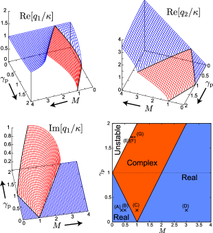
Figure 1: (Color online) Real and imaginary parts of $q_{1}/\kappa$ and $q_{2}/\kappa$ in the plane of $\gamma_{\rm p}$ and $M=1/\kappa{\bar{\xi}}$ in the linear theory. Here $q_{1}$ and $q_{2}$ are positive for $\gamma_{\rm p}<|M-1|$ (in blue) and are complex conjugates for $|M-1|<\gamma_{\rm p}<M+1$ (in red), while the system is unstable for $\gamma_{\rm p}>M+1$ (in white). These three regions are depicted in the right bottom panel, where the profiles and the interaction free energy will be shown at four $\times$ points (A), (B), (C) and (D) in Fig.2 and those at three $\bullet$ points (E), (F), and (G) in Fig.3 in the linear theory.

III.3 Profiles around a single colloid particle

In the presence of a single colloid with radius $a$, we obtain the fundamental profiles $U=U_{0}(r)$ and $\psi=\psi_{0}(r)$ induced by nonvanishing $\bar{\gamma}$ and $\bar{\sigma}$ from the boundary conditions (3.12) and (3.13). In the large system limit $V\gg a^{3}$, they are expressed as linear combinations of two Yukawa functions, $e^{-q_{1}(r-a)}/r$ and $e^{-q_{2}(r-a)}/r$, where $r$ is the distance from the colloid center. As will be shown in Appendix B, they are of the forms,

$$U_{0}=\frac{g_{a}B_{1}e^{-q_{1}(r-a)}}{(1-\lambda_{1})(1+q_{1}a)r}-\frac{g_{a}B_{2}e^{-q_{2}(r-a)}}{(1-\lambda_{2})(1+q_{2}a)r},$$

$$\psi_{0}=\frac{B_{1}e^{-q_{1}(r-a)}}{(1+q_{1}a)r}-\frac{B_{2}e^{-q_{2}(r-a)}}{(1+q_{2}a)r}.$$ (3.25)

The coefficients $B_{1}$ and $B_{2}$ are defined by

$$B_{i}=a^{2}[{\bar{\gamma}(1-\lambda_{i})-\bar{\sigma}g_{a}}]/{C}({\lambda_{1}-\lambda_{2}}).$$ (3.26)

In Appendix A, we will also express the correlation functions of the composition and the ion densities as linear combinations of these Yukawa functions.

We examine some limiting cases. (i) As $g_{a}\to 0$, we find $\lambda_{1}\to 1$, $\lambda_{2}\to M^{2}$, and

$$U_{0}\cong{\bar{Q}}\frac{\ell_{B}e^{-\kappa(r-a)}}{(1+\kappa a)r},\quad\psi_{0}\cong-{{\bar{\gamma}}}\frac{a^{2}e^{-(r-a)/{\bar{\xi}}}}{C(1+a/{\bar{\xi}})r},$$ (3.27)

where $U_{0}$ is the Debye-H$\ddot{\rm u}$ckel form Russel ; LevinReview ; Dej ; Ov with ${\bar{Q}}$ being the average charge of a colloid particle,

$${\bar{Q}}=-4\pi a^{2}{\bar{\sigma}}e.$$ (3.28)

(ii) We assume $|q_{i}|a\ll 1$ and $|q_{i}|(r-a)\ll 1$, which hold in the limit of small $q_{i}$. Even for $g_{a}\neq 0$, Eq.(3.25) yields the Coulombic behavior,

$$U_{0}\cong{\bar{Q}}{\ell_{B}}\frac{1}{r},\quad\psi_{0}\cong-({\bar{\gamma}}{a^{2}}/{C})\frac{1}{r},$$ (3.29)

which follow from the relations $B_{1}-B_{2}=-{\bar{\gamma}}a^{2}/C$ and $B_{1}/(1-\lambda_{1})-B_{2}/(1-\lambda_{2})=-4\pi\ell_{B}{\bar{\sigma}}a^{2}/g_{a}$. (iii) Let us approach the instability line $M=\gamma_{\rm p}-1$ in Fig.1. In this case, both $U_{0}$ and $\psi_{0}$ grow as Im$[(\lambda_{1}-\lambda_{2})^{-1}]=-1/2q_{I}q_{R}\propto(M-\gamma_{\rm p}+1)^{-1/2}$. In this limit, the linear theory is valid only for very small $\bar{\sigma}$ and $\bar{\gamma}$.

III.4 Interaction between two colloid particles

We suppose two colloid particles of the same species with radius $a$. In Appendix B, we will derive the interaction free energy $F_{\rm int}$ from $\Delta\Omega$ in Eq.(3.17) as a linear combination of two Yukawa functions, $e^{-q_{1}(d-2a)}/d$ and $e^{-q_{2}(d-2a)}/d$, where $d$ is the separation distance between the two colloid centers longer than $2a$. We express it as

$$\frac{F_{\rm int}}{T}={4\pi a^{4}}\bigg{[}\frac{E_{1}e^{-q_{1}(d-2a)}}{(1+q_{1}a)^{2}d}-\frac{E_{2}e^{-q_{2}(d-2a)}}{(1+q_{2}a)^{2}d}\bigg{]},$$ (3.30)

where the coefficients $E_{1}$ and $E_{2}$ are defined by

$$E_{i}=\frac{[\bar{\gamma}(1-\lambda_{i})-\bar{\sigma}g_{a}]^{2}}{C(1-\lambda_{i})(\lambda_{1}-\lambda_{2})}.$$ (3.31)

Notice that $F_{\rm int}$ is independent of the colloid dielectric constant $\varepsilon_{\rm p}$. In Appendix B, we can see that $\varepsilon_{\rm p}$ appears in the third order contribution.

Some limiting cases are as follows. (i) In the limit of weak solvation $g_{1}\to 0$ and $g_{2}\to 0$, we have $E_{1}\to 4\pi\ell_{B}{\bar{\sigma}}^{2}$ and $E_{2}\to{\bar{\gamma}}^{2}/C$, leading to a decoupled expression,

$${F_{\rm int}} = F_{\rm DLVO}+F_{\rm ad}$$ (3.32)

$$=\frac{{\bar{Q}}^{2}e^{-\kappa(d-2a)}}{\bar{\varepsilon}(1+\kappa a)^{2}d}-4\pi\frac{Ta^{4}\bar{\gamma}^{2}e^{-(d-2a)/{\xi}}}{C(1+a/{\xi})^{2}d}.$$

The first term is the DLVO interaction $F_{\rm DLVO}$ in Eq.(1.2) LevinReview ; Dej ; Ov ; Russel . The second term represents the adsorption-induced attraction $F_{\rm ad}$ for small $\bar{\gamma}$. For neutral colloids, we have $\bar{\gamma}=\gamma$ and $h_{1}=-T\gamma$ to find the expression (1.5) with $A_{\rm ad}=4\pi T{\gamma^{2}}/C$. Note that the linear theory is not applicable very close to the criticality h1 , as stated below Eq.(1.5). (ii) When $|q_{i}|a\ll 1$ and $|q_{i}|(d-2a)\ll 1$, we use $E_{1}-E_{2}={4\pi\ell_{B}}{\bar{\sigma}}^{2}-{{\bar{\gamma}}^{2}}/{C}$ to obtain

$${F_{\rm int}}\cong 4\pi Ta^{4}({4\pi\ell_{B}}{\bar{\sigma}}^{2}-{{\bar{\gamma}}^{2}}/{C})/d.$$ (3.33)

(iii) Near the criticality and for hydrophilic ions, we may assume $M\ll 1$ and $1-\gamma_{\rm p}^{2}\gg M$, where $q_{1}$ and $q_{2}$ are given by Eq.(3.23). Then ${F_{\rm int}}$ in Eq.(3.30) takes the same form as the decoupled expression (3.32):

$${F_{\rm int}}=\frac{{\bar{Q}}_{e}^{2}e^{-q_{1}(d-2a)}}{\bar{\varepsilon}(1+q_{1}a)^{2}d}-4\pi\frac{Ta^{4}\bar{\gamma}_{e}^{2}e^{-q_{2}(d-2a)}}{C(1+q_{2}a)^{2}d}.$$ (3.34)

where ${\bar{Q}}$ and $\bar{\gamma}$ in Eq.(3.32) have been replaced by ${\bar{Q}}_{e}$ and $\bar{\gamma}_{e}$ defined by

$${\bar{Q}}_{e}={\bar{Q}}(1-g_{a}{\bar{\gamma}}/4\pi C\ell_{B}{\bar{\sigma}})/\sqrt{1-\gamma_{\rm p}^{2}},$$

$$\bar{\gamma}_{e}=({\bar{\gamma}}-{\bar{\sigma}}g_{a})/\sqrt{1-\gamma_{\rm p}^{2}}.$$ (3.35)

(v) When $q_{1}$ and $q_{2}$ are complex conjugates in the region $|M-1|<\gamma_{\rm p}<M+1$ in Fig.1, Eq.(3.30) gives

$${F_{\rm int}}=8\pi Ta^{4}\exp[{-q_{R}(d-2a)}]\frac{1}{d}$$

$$\times\{J\cos[q_{I}(d-2a)]+K\sin[q_{I}(d-2a)]\},$$ (3.36)

where the coefficients $J$ and $K$ are the real and imaginary parts of $E_{1}/(1+q_{1}a)^{2}$. On approaching the spinodal line $\gamma_{\rm p}=M+1$, $K$ grows as $1/q_{R}$ but $J$ remains finite.

For neutral colloids, we compare the van der Waals interaction $F_{\rm vdw}(d)$ in Eq.(1.2) and the adsorption-induced interaction $F_{\rm ad}(d)$ in Eq.(1.5) or (3.32) at the closest separation $d-2a=a_{0}$, where $\bar{\gamma}=\gamma$ and $\bar{\xi}=\xi$. If $C\sim a_{0}^{-1}$ comment-gra , we estimate their ratio as

$$\frac{F_{\rm ad}}{F_{\rm vdw}} \sim 10^{2}(a_{0}a\gamma)^{2}T/{A_{H}}\quad(a\gg\xi)$$ (3.37)

$$\sim 10^{2}(a_{0}\xi\gamma)^{2}T/{A_{H}}\quad(a\ll\xi).$$

Even at the closest separation, the van der Waals attraction is negligible when $A_{H}/T$ is smaller than $(10a_{0}a\gamma)^{2}$ for $a\gg\xi$ and than $(10a_{0}\xi\gamma)^{2}$ for $a\ll\xi$.

III.5 Plotting analytic results in the linear theory

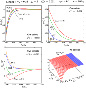
Figure 2: (Color online) Results of the linear theory with $a=600a_{0}$ for hydrophilic ions with $\gamma_{\rm p}=0.23$, $g_{a}=2$, $\bar{\sigma}=0.001a_{0}^{-2}$, and $\kappa=0.1a_{0}^{-1}$, where $M$ is (A) 0.4, (B) 0.5, (C) 1, and (D) 3 (see Fig.1 for their locations in the $M$-$\gamma_{\rm p}$ plane). Top: Normalized potential $U_{0}(r)$ (left) and composition deviation $\psi_{0}(r)$ (right) in Eq.(3.25) vs $r/a_{0}$ around a colloid. Left bottom: Interaction free energy $F_{\rm int}(d)$ between two colloids in Eq.(3.30) vs $d/a_{0}$. Right bottom: Minimum of $F_{\rm int}$, denoted by $F_{\rm int}^{\rm min}$, in the $M$-$\bar{\gamma}/\bar{\sigma}$ plane with the common $\bar{\sigma}$, $\kappa$, and $a$. It is zero (attained at infinity) in the right (for $M\gtrsim 1.3)$ and is negative in the left (for smaller $M$).

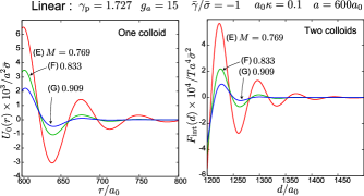
Figure 3: (Color online) Results of the linear theory with $a=600a_{0}$ for antagonistic ions with $\gamma_{\rm p}=1.727$, $g_{a}=15$, $\bar{\gamma}/\bar{\sigma}=-1$, and $\kappa=0.1a_{0}^{-1}$, where $M$ is (E) 0.769, (F) 0.833, and (G) 0.909 (see Fig.1 for their locations). Left: Normalized potential $U_{0}(r)/a^{2}{\bar{\sigma}}$ vs $r/a_{0}$ around a colloid. Right: Normalized interaction free energy $F_{\rm int}(d)/a^{4}{\bar{\sigma}}^{2}$ between two colloids from Eq.(3.30) vs $d/a_{0}$.

On the basis of the analytic expressions (3.25) and (3.30), we plot $U_{0}(r)$ and $\psi_{0}(r)$ around a single colloid and $F_{\rm int}$ between two colloids for various $M$. Assuming a large radius $a=600a_{0}$, we set $\ell_{B}=3a_{0}$ and $\kappa=0.1a_{0}^{-1}$, where $a_{0}=v_{0}^{1/3}$. Then $n_{0}=1.33\times 10^{-4}v_{0}^{-1}$.

In Fig.2, with hydrophilic ions, we set $\gamma_{\rm p}=0.23$, $g_{a}=2$, $\bar{\sigma}=0.001a_{0}^{-2}$, and $\bar{\gamma}/\bar{\sigma}=-2$. We can see that $\psi_{0}$ increases considerably with decreasing $M$, while $U_{0}$ is rather insensitive to $M$. Remarkably, the curves of $F_{\rm int}$ vs $d/a$ exhibit a negative minimum at an intermediate $d$ for small $M$. With these selected parameters, the DLVO interaction $F_{\rm DLVO}$ is equal to $1.061\times 10^{-4}Ta^{4}{\bar{\sigma}}^{2}=13.75T$ at $d=2a_{0}$.

In Fig.3, with antagonistic ions Nara ; Current ; Sadakane , we display $U_{0}(r)/a^{2}{\bar{\sigma}}$ and $F_{\rm int}(d)/Ta^{4}{\bar{\sigma}}^{2}$ by setting $\gamma_{\rm p}=1.727$, $g_{a}=15$, and $\bar{\gamma}/\bar{\sigma}=-1$. As $M\to M_{c}=0.727$, $U_{0}(r)$ and $F_{\rm int}(d)$ grow as stated below Eqs.(3.24) and (3.36). Oscillatory relaxation is conspicuous close to the instability. Here, the linear conditions, $|U_{0}|\ll 1$ and $|\psi_{0}|\ll 1$, are ensured only by very small $\bar{\sigma}$ and $\bar{\gamma}$. Otherwise, the nonlinear theory is required. In Fig.3, we thus divide $U_{0}$ and $F_{\rm int}$ by $a^{2}{\bar{\sigma}}$ and $a^{4}{\bar{\sigma}}^{2}$, respectively.

IV Precipitation due to highly selective solvation

In a binary mixture in one-phase states, a highly selective solute can induce precipitation of domains rich in the preferred component Okamoto ; Current . The solute can be either a hydrophilic salt (such as NaCl) or a neutral hydrophobic solute. The equilibrium size of a precipitated domain depends on the system size $V$ (as can be known from Eq.(4.8) below).

In the next section, we will show numerically that precipitation can occur on the colloid surface. Therefore, in this section, we summarize and extend our previous theory Okamoto to understand precipitation on the colloid surface. We suppose an experiment of very dilute colloid suspension; then, the volume $V$ assigned to each colloid particle is the inverse droplet density $n_{D}^{-1}$. For high colloid concentrations, colloids should interact collectively due to the growth of wetting layers to form a floccuated phase Beysens ; Guo ; Kaler .

IV.1 Bulk precipitation

For hydrophilic cations and anions, the phase behavior of precipitation is little affected by charge density variations, because they are significant only at interfaces, colloid surfaces, or a container (see the right bottom panel of Fig.10 as an example). Thus, neglecting the electrostatic interaction, we may use results of a three component system Okamoto by setting

$$n_{1}=n_{2}=n/2,$$ (4.1)

$$g=(g_{1}+g_{2})/2.$$ (4.2)

We assume the strong solvation condition $g\gg 1$. In the precipitated phase, called $\alpha$, the water composition $\phi_{\alpha}$ is close to unity and the solute density $n_{\alpha}$ is much larger than the average ${\bar{n}}=2n_{0}$ by the factor $e^{g(1-{\bar{\phi}})}$ largefactor . The precipitation effect is significant for not small $g(1-{\bar{\phi}})$.

Let us decrease $\bar{n}$ in the presence of precipitated domains. Then the volume fraction $\gamma_{\alpha}$ of phase $\alpha$ decreases and eventually tends to zero as

$$\gamma_{\alpha}=({\bar{n}}/n_{\rm p}-1)e^{-g(1-\bar{\phi})},$$ (4.3)

where $n_{\rm p}$ is a minimum solute density for precipitation. Its asymptotic expression for $g\gg 1$ is given by

$$n_{\rm p}=e^{-g(1-\bar{\phi})}G({\bar{\phi}},\chi)/T.$$ (4.4)

The function $G({\bar{\phi}},\chi)$ is a positive quantity defined by

$$G({\bar{\phi}},\chi) = -f(\bar{\phi})-(1-\bar{\phi})f^{\prime}(\bar{\phi})$$ (4.5)

$$= -(T/v_{0})[\ln\bar{\phi}+\chi(1-\bar{\phi})^{2}],$$

where the second line follows from Eq.(2.4). Alternatively, we may decrease $\chi$ at fixed $\bar{\phi}$ and ${\bar{n}}$ in the presence of precipitated domains. The volume fraction $\gamma_{\alpha}$ tends to zero as $\chi$ approaches a lower bound $\chi_{\rm p}=\chi_{\rm p}(\bar{\phi},{\bar{n}})$. From Eq.(4.4), $\chi_{\rm p}$ satisfies ${\bar{n}}=e^{-g(1-\bar{\phi})}G({\bar{\phi}},\chi_{\rm p})/T.$ Use of the second line of Eq.(4.5) gives

$$\chi_{\rm p}=-[\ln{\bar{\phi}}+e^{g(1-\bar{\phi})}v_{0}{\bar{n}}]/(1-{\bar{\phi}})^{2}.$$ (4.6)

It also follows the relation,

$$\chi-\chi_{\rm p}\cong v_{0}e^{g(1-{\bar{\phi}})}({\bar{n}}-n_{\rm p})/(1-{\bar{\phi}})^{2}.$$ (4.7)

Here $\bar{n}$ appears in the combination $e^{g(1-\bar{\phi})}{\bar{n}}$.

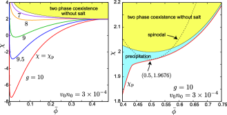
Figure 4: (Color online) Minimum interaction parameter $\chi_{\rm p}$ vs $\bar{\phi}$ at ${n}_{0}=3\times 10^{-4}v_{0}^{-1}$ in the range $0<{\bar{\phi}}<0.47$ for $g=7,8,8.5,9$, 9.5, and 10 from above (left) and in the range $0.4<{\bar{\phi}}<0.75$ for $g=10$ (right). Two-phase coexistence region (in yellow) without solute is in the upper part. Spinodal curve $\tau=\tau_{c}$ is also written by dotted line (right).

In Fig.4, we display $\chi_{\rm p}$ vs $\bar{\phi}$ at ${n}_{0}=3\times 10^{-4}v_{0}^{-1}$. The left panel gives the curves for $g=7,8,8.5,9$, 9.5, and 10 in the range $0<{\bar{\phi}}<0.47$. With increasing $g$, the precipitation branch is suddenly detached downward from the solvent coexistence curve. For $g\gg 1$, they are in excellent agreement with the asymptotic formula (4.6) for $\chi_{\rm p}$. (The asymptotic formula (4.4) for $n_{\rm p}$ is also a good approximation for $g\gg 1$ Okamoto ; Current .) The right panel gives the curve for $g=10$ at the same $n_{0}$ in the range $0.4<{\bar{\phi}}<0.75$. The curve is only slightly outside the coexistence curve for ${\bar{\phi}}\gtrsim 0.6$ and touches the spinodal curve $\tau=\tau_{c}$ at $(\chi,{\bar{\phi}})=(0.5187,1.9728)$ touch . We obtained these curves numerically from minimization of the bulk free energy at $\langle{\phi}\rangle={\bar{\phi}}$ and $\langle{n}\rangle={\bar{n}}$, neglecting the surface free energy. Thus these curves are those for two-phase coexistence with a planar interface separating the two phases.

IV.2 Surface tension effect on a precipitated droplet

The surface tension $\sigma_{s}$ between a precipitated droplet and the surrounding solute-poor region is well-defined, though the precipitation is a nonlinear effect of a highly selective solute. It is of order $\sigma_{s}\sim T/a_{0}^{2}$ far from the solvent criticality, being independent of the solute density. We here examine the surface tension effect on the droplet stability.

We consider a single spherical droplet of phase $\alpha$ with radius $R$ in a large volume $V$. The droplet volume fraction is then $\gamma_{\alpha}=v/V$, where $v=4\pi R^{3}/3$. For $\bar{n}>n_{\rm p}$ and at very small volume fraction $\gamma_{\alpha}\ll e^{-g(1-\bar{\phi})}$, the droplet free energy is expressed as comment1 ; Binder

$${\Delta F}=4\pi\sigma_{s}{R^{2}}-T(\bar{n}-n_{\rm p})e^{g(1-\bar{\phi})}v+\frac{T{\bar{n}}}{2V}e^{2g(1-\bar{\phi})}v^{2}$$

$$=4\pi\sigma_{s}(R^{2}-2R^{3}/3R_{c}+R^{6}/3R_{\rm m}^{4}).$$ (4.8)

In the first line, the first two terms constitute the standard droplet free energy in the nucleation theory and the third term ($\propto R^{6}/V$) arises from the finite size effect Onukibook . In the second line, we introduce a critical radius $R_{c}$ and a minimum radius $R_{\rm m}$ by

$$R_{c}=2\sigma_{s}e^{-g(1-\bar{\phi})}/T(\bar{n}-n_{\rm p})$$

$$~{}~{}~{}=2v_{0}\sigma_{s}/[T(1-{\bar{\phi}})^{2}(\chi-\chi_{\rm p})],$$ (4.9)

$$R_{\rm m}=(3\sigma_{s}V/2\pi T{\bar{n}})^{1/4}e^{-g(1-\bar{\phi})/2}.$$ (4.10)

where Eq.(4.7) is used in the second line of Eq.(4.9), $R_{c}$ grows as $\chi\to\chi_{\rm p}$, and $R_{\rm m}$ decreases with decreasing $\bar{\phi}$. We estimate $R_{\rm m}\sim(Va_{0}/v_{0}{\bar{n}})^{1/4}e^{-g(1-{\bar{\phi}})/2}$ far from the solvent criticality. Minimization of the second line of Eq.(4.8) yields

$$(R/R_{\rm m})^{4}=R/R_{c}-1>0$$ (4.11)

for the equilibrium radius $R$. We require $\Delta F/4\pi\sigma_{s}R^{2}=(2-R/R_{c})/3<0$ to find $R>2R_{c}$. Hence $R>R_{\rm m}$ from Eq.(4.11) and $R_{\rm m}$ is the minimum radius of equilibrium droplets in a finite system comment1 . For $R_{\rm m}\gg R_{c}$, droplets with radii much larger than $R_{\rm m}$ can appear as

$$R^{3}\cong R_{\rm m}^{4}/R_{c},$$ (4.12)

where the right hand side is proportional to $V$ and is independent of $\sigma_{s}$ in agreement with Eq.(4.3).

It also follows the condition $R_{\rm m}>2R_{c}$ from Eq.(4.11) comment2 , leading to lower bounds of ${\bar{n}}-n_{\rm p}$ and $\chi-\chi_{\rm p}$ as

$${\bar{n}}-n_{\rm p}>4\sigma_{s}e^{-g(1-\bar{\phi})}/TR_{\rm m},$$ (4.13)

$$\chi-\chi_{\rm p}>4v_{0}\sigma_{s}/TR_{\rm m}(1-\bar{\phi})^{2},$$ (4.14)

for the formation of a droplet. Thus the bulk precipitation curves ${\bar{n}}=n_{\rm p}$ and ${\chi}=\chi_{\rm p}$ are shifted upward by amounts proportional to $\sigma_{s}/R_{\rm m}\propto\sigma_{s}^{3/4}V^{-1/4}$ for droplets with surface tension.

As an example, let us set $V=4\times 10^{9}\pi a_{0}^{3}/3$ with $C=2a_{0}^{-1}$, $g=10$, $\bar{n}=6\times 10^{-4}v_{0}^{-1}$, and $\bar{\phi}=0.41$. The surface tension is then $\sigma_{s}=0.06T/a_{0}^{2}$ as $\chi\to\chi_{\rm p}=1.871$ Okamoto . Thus we obtain $n_{\rm p}=6\times 10^{-4}$ and $R_{\rm m}=35.1a_{0}$. The right hand side of Eq.(4.13) is $1.9\times 10^{-5}$, while that of Eq.(4.14) is $0.02$.

IV.3 Wetting layer formation on a colloid surface

A completely wetting layer can appear on a colloid surface above a precipitation curve for the hydrophilic case $\gamma<0$ or for the hydrophobic case $\gamma>0$ under the condition (2.29). In our numerical analysis, the precipitation curve for a colloid is only slightly shifted upward from the bulk curve $\chi=\chi_{\rm p}$ in the $\chi$-$\bar{\phi}$ plane. We also recognize that the precipitation curve is nearly independent of the surface parameters $\gamma$ and $\sigma_{0}$ (see Figs.6 and 8).

We suppose that a colloid with radius $a$ is completely wetted by a spherically symmetric layer with thickness $R-a$. The volume fraction of phase $\alpha$ is $\gamma_{\alpha}=4\pi(R^{3}-a^{3})/3V$ in a volume $V$. For $R-a\gg a_{0}$, we may treat the surface free energy between the colloid surface and the wetting layer as a constant. As a generalization of Eq.(4.8), $R$ is determined by minimization of a free energy contribution $F_{\rm wet}$. In terms of $R_{c}$ in Eq.(4.9) and $R_{\rm m}$ in Eq.(4.10), it is expressed as

$$\frac{F_{\rm wet}}{4\pi\sigma_{s}}=R^{2}-a^{2}-\frac{2}{3R_{c}}(R^{3}-a^{3})+\frac{1}{3R_{\rm m}^{4}}(R^{3}-a^{3})^{2}$$

$$\hskip 11.38092pt={R_{\rm m}^{2}}\bigg{[}(q+s^{3})^{2/3}-s^{2}-\frac{2R_{\rm m}}{3R_{c}}q+\frac{q^{2}}{3}\bigg{]}.$$ (4.15)

The first line tends to Eq.(4.8) as $a\to 0$. In the second line, $q$ and $s$ are defined by

$$q = (R^{3}-a^{3})/R_{\rm m}^{3},$$ (4.16)

$$s = a/R_{\rm m}.$$ (4.17)

We treat $q$ as an order parameter. In Eq.(4.15), the selective solvation is accounted for in $R_{c}$ and $R_{\rm m}$, but the electrostatic interaction is neglected. See Fig.18 in Ref.Okamoto for $q$ in the $s$-$R_{\rm m}/R_{c}$ plane (where $s$ in Eq.(4.17) is written as $D$). In the thin layer limit $R^{3}/a^{3}-1\ll 1$ or for $q\ll s^{3}$, $F_{\rm wet}$ is expanded up to the third order with respect to $q$ as

$$\frac{F_{\rm wet}}{4\pi\sigma_{s}R_{\rm m}^{2}}={(1-\frac{a}{R_{c}})}\frac{2q}{3s}+({3}-\frac{1}{s^{4}})\frac{q^{2}}{9}+\frac{4q^{3}}{81s^{7}}.$$ (4.18)

Here the coefficients of the first two terms can vanish at $a/R_{c}=1$ and $s=3^{-1/4}$, where we predict tricritical behavior with varying $\chi$ or $R_{c}$. That is, $q$ changes continuously or discontinuously depending on whether $a>3^{-1/4}R_{\rm m}$ or $a<3^{-1/4}R_{\rm m}$.

For $a>3^{-1/4}R_{\rm m},$ $q$ becomes nonvanishing for $1-a/R_{c}<0$ or for $R_{c}^{-1}>a^{-1}$ continuously as a second-order phase transition. From Eq.(4.9) this condition yields a lower bound of $\chi-\chi_{\rm p}$ in the form,

$$\chi-\chi_{\rm p}>2v_{0}\sigma_{s}/Ta(1-\bar{\phi})^{2},$$ (4.19)

which also follows if $R_{\rm m}$ is replaced by $2a$ in Eq.(4.14). With further increasing $a$ much above $R_{\rm m}$ or for $s\gg 1$, the first two terms in Eq.(4.18) gives $q\cong(a/R_{c}-1)/s$ or

$$R^{3}/a^{3}-1\cong(R_{\rm m}/a)^{4}(a/R_{c}-1),$$ (4.20)

which holds for $a/R_{c}-1\ll(a/R_{\rm m})^{4}$ because we have assumed $q\ll s^{3}$ in setting up Eq.(4.18). The situation $a\gg R_{\rm m}$ can well happen in real systems particularly for relatively small $\bar{\phi}$ (where $R_{\rm m}$ is decreased). In such cases, the factor $(R_{\rm m}/a)^{4}$ in Eq.(4.20) is small and the wetting layer thickens slowly with increasing $\chi$. On the other hand, in the thick layer limit $R\gg a$, $R$ is given by Eq.(4.12).

For $a<3^{-1/4}R_{\rm m},$ $q$ becomes nonvanishing discontinuously as a first-order phase transition when $1-a/R_{c}$ is smaller than a small positive constant ($\propto(s-3^{-1/4})^{2}$ near the tricriticality). As a result, the lower bound of $\chi-\chi_{\rm p}$ for precipitation is slightly smaller than the right hand side of Eq.(4.19).

In the above theory, we have examined the transition between weakly adsorbed states and completely wetted states. In the next section, however, we shall see that a hydrophobic surface can be partially wetted by a nonspherical water-rich layer at relatively small $\bar{\phi}$ and for not very large $\gamma$ (see Figs.16 and 17).

V Numerical results

In this section, we present numerical results on the basis of our nonlinear theory in Sec.II with a single colloid or two colloids placed at the center of a large cell. The correlation length $\bar{\xi}$ in Eq.(3.11) increases up to $14.1a_{0}$ at $\chi=1.965$ in Fig.12, but it is only a few times longer than $a_{0}$ in the other examples far from the solvent criticality.

V.1 Parameter values selected

We set $C=2a_{0}^{-1}$, $\Delta_{0}=18$, $\Delta_{1}=12$, $\ell_{B}=e^{2}/\varepsilon_{0}k_{B}T=3a_{0}$, and $\varepsilon_{1}=\varepsilon_{0}$. We use large $\Delta_{1}$, so the degree of ionization $\alpha$ sensitively depends on the surface composition from Eq.(2.25). Several values are assigned to the density of ionizable groups. surface with $\gamma>0$. Because of the numerical convenience, the colloid radius $a$ is assumed to be rather small as

$$a=15a_{0}.$$ (5.1)

We also performed simulations with $a=25a_{0}$ to obtain essentially the same results, though the corresponding figures are not shown.

In Subsecs.VB-D, we treat hydrophilic ions with $g_{1}=11$ and $g_{2}=9$ at $v_{0}{n}_{0}=3\times 10^{-4}$ in Figs.5-17. Recall that we have introduced the Debye wavenumber $\kappa$ in Eq.(3.5) and the asymmetry parameter $\gamma_{\rm p}$ in Eq.(3.22) as functions of the average composition $\bar{\phi}$. Here, we have $\kappa=0.127a_{0}^{-1}$ and $\gamma_{\rm p}=0.135$ for $\bar{\phi}=0.4$. In Subsec.VE, we treat antagonistic ion pairs with $g_{1}=-g_{2}=13$ at $v_{0}{n}_{0}=10^{-3}$ in Figs.18 and 19, where we have $\kappa=0.233a_{0}^{-1}$ and $\gamma_{\rm p}=1.76$ for $\bar{\phi}=0.4$.

In the case of a single colloid, our cell is a large sphere with radius $10^{3}a_{0}$ in the spherically symmetric geometry. In the case of two colloids, it is a cylinder with radius $256a_{0}$ and height $512a_{0}$ in the axisymmetric geometry. Since $a=15a_{0}$, the colloid volume fraction is $3.375\times 10^{-6}$ for a single colloid and is $1.341\times 10^{-4}$ for two colloids. For hydrophilic ions and at $\bar{\phi}=0.41$, $R_{\rm m}$ in Eq.(4.10) is $35.1a_{0}$ in the single colloid case largefactor and $13.0a_{0}$ in the two colloid case. In agreement with the discussion in Subsec.IVC, the layer formation due to precipitation is discontinuous for the single colloid case (where $a<3^{-1/4}R_{\rm m}$) but is continuous for the two colloid case (where $a>3^{-1/4}R_{\rm m}$).

V.2 Comparison of the linear and nonlinear theories

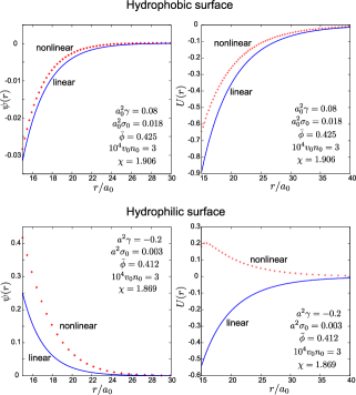
Figure 5: (Color online) $\psi(r)=\phi(r)-{\bar{\phi}}$ and $U(r)$ vs $r/a_{0}$ around a colloid from the linear and nonlinear theories below the precipitation line at $v_{0}{n}_{0}=3\times 10^{-4}$. Upper plates: Those for a hydrophobic surface with $\gamma=0.08a_{0}^{-2}$ at $\sigma_{0}=0.018a_{0}^{-2}$, where $|\psi|$ at the surface is smaller than $1/g_{i}$ and $|U|$ is at most of order unity so that the linear results fairly agree with the nonlinear results. Lower plates: Those for a hydrophilic surface with $\gamma=0.2a_{0}^{-2}$ at small $\sigma_{0}=0.003a_{0}^{-2}$. From $\psi\sim 0.3$ as $r\to a$, the cations are considerably accumulated near the surface and $U$ becomes positive in the nonlinear theory, while $U$ remains negative in the linear theory.

We compare the profiles of $\psi(r)=\phi(r)-{\bar{\phi}}$ and $U(r)=e\Phi(r)/T$ from the linear theory in Sec.III and those from the nonlinear theory in Sec.II below the bulk precipitation curve $\chi<\chi_{\rm p}$. The linear theory is based on the assumptions (3.2) and (3.3) and is thus valid only for $|\psi|\lesssim 1/|g_{i}|$ and $|U|\lesssim 1$ near the surface.

In the upper plates of Fig.5, we suppose hydrophilic ions and a hydrophobic surface with $\gamma=0.08a_{0}^{-2}$. The other parameters are $\chi=1.908$, $\bar{\phi}=0.425$, and ${\sigma}_{0}=0.018a_{0}^{-2}$. Here $\alpha=0.25$ from the nonlinear calculation, leading to ${\bar{\sigma}}=0.0045$ and ${\bar{\gamma}}=0.026$, which were then used in the linear calculation. In this case, $g_{i}\phi$ and $U$ are both decreased near the surface and their amplitudes are not large compared to unity. Thus the linear results are in fair agreement with the nonlinear results.

In the lower plates of Fig.5, we suppose hydrophilic ions and a hydrophilic surface with $\gamma=-0.2a_{0}^{-2}$. The other parameters are $\chi=1.869$, $\bar{\phi}=0.412$, and ${\sigma}_{0}=0.003a_{0}^{-2}$. We have $\alpha=0.992$ in the nonlinear calculation, which gives ${\bar{\sigma}}=0.00297a_{0}^{-2}$ and ${\bar{\gamma}}=-0.236a_{0}^{-2}$. In this case, $\phi$ is a few times larger than $1/g_{i}\sim 0.1$ near the surface, leading to considerable ion accumulation, which cannot be accounted for in the linear theory. Furthermore, the cations are more enriched than the anions near the surface, leading to positive $U$ in the nonlinear theory, while $U$ remains negative in the linear theory.

Comparison of the linear and nonlinear theories will also be made in the presence of two colloids at $\bar{\phi}=0.5$. See explanations of Fig.12 below.

V.3 Prewetting and precipitation on a colloid

With hydrophilic ions, there appear two transition lines of prewetting and precipitation for each colloid in the ${\bar{\phi}}$-$\chi$ plane. They are located far below the solvent coexistence curve for strong selective solvation. The prewetting line sensitively depends on $\gamma$ and $\sigma_{0}$ (as will be seen in Figs.6 and 8 below). It starts from a point on the precipitation line ending at a surface critical point, across which there are discontinuities in the physical quantities. The transition across the precipitation line for a colloid is first-order for the present parameters. We further confirmed that the precipitation line exhibits no appreciable dependence on $\gamma$ and $\sigma_{0}$ and approaches the bulk one $\chi=\chi_{\rm p}$ with increasing $a$ for $a<3^{-1/4}R_{\rm m}$. If $a>3^{-1/4}R_{\rm m}$, the precipitation transition becomes continuous and it is difficult to precisely determine the location of the precipitation line.

V.3.1 Hydrophilic surface with $\gamma=-0.2a_{0}^{-2}$

In our previous workOkamoto , we examined one example of a hydrophilic colloid with $\gamma=-0.2a_{0}^{-2}$ in the presence of hydrophilic ions, where precipitation and prewetting are first induced on the colloid surface before in the bulk region. Again with $\gamma=-0.2a_{0}^{-2}$, the left panel of Fig.6 displays three examples of the prewetting line corresponding to $a^{2}\sigma_{0}=0$, 0.003, and 0.005, around which $\alpha$ is nearly equal to unity and $\sigma\cong\sigma_{0}$. A first-order precipitation line is also shown (broken line), which is independent of $\sigma_{0}$. The right panel of Fig.6 shows the preferential adsorption $\Gamma$ around a colloid as a function of $\chi$ for several $\bar{\phi}$ at $a^{2}\sigma_{0}=003$. Since $\phi(r)$ tends to a constant $\phi(L)$ far from the colloid, $\Gamma$ is calculated from

$$\Gamma=\int^{\prime}d{\mbox{\boldmath$r$}}[\phi({\mbox{\boldmath$r$}})-{\phi}(L)],$$ (5.2)

where the integration is in the colloid exterior. With precipitation, we have $\Gamma\sim 4\pi(1-{\bar{\phi}})(R^{3}-a^{3})/3$ for a single colloid.

In Fig.7, profiles of $\phi(r)$ and the total ion density $n_{1}(r)+n_{2}(r)$ are displayed at four points (A)-(D) marked in Fig.6, where $\gamma=-0.2a_{0}^{-2}$, $\bar{\phi}=0.412$, and $\sigma_{0}=0.003a_{0}^{-2}$. We can see a weakly discontinuous prewetting transition between (A) and (B) and a strongly discontinuous precipitation transition between (C) and (D). The value of $\chi$ at this precipitation transition is 1.8945, while it is $1.8926$ for $d=25a_{0}$ with the other parameters held at the same values (not shown here). These values of $\chi$ are slightly larger than $\chi_{\rm p}=1.8795$ at $\bar{\phi}=0.412$.

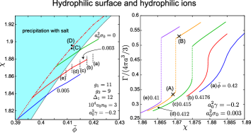
Figure 6: (Color online) Prewetting and precipitation transitions on a hydrophilic colloid surface with $a=15a_{0}$ and $\gamma=-0.2a_{0}^{-2}$. Left:Colloidal precipitation line (red broken line) and prewetting lines for $a_{0}^{2}\sigma_{0}=0$, 0.003, and 0.005, around which $\alpha\cong 1$ here. Right: Normalized adsorption $\Gamma/(4\pi a^{3}/3)$ vs $\chi$ at $a_{0}^{2}\sigma_{0}=0.003$ for (a) $\bar{\phi}=0.42$, (b) 0.4176, (c) 0.415, (d) 0.412, and (e) 0.41. No phase transition appears on path (a), the prewetting critical point is on path (b), and the transition is discontinuous for paths (c), (d), and (e).

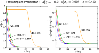
Figure 7: (Color online) $\phi(r)$ (left) and $v_{0}(n_{1}(r)+n_{2}(r))$ (right) at four points (A)-(D) marked in Fig.6 for a hydrophilic colloid surface with $\gamma=-0.2a_{0}^{-2}$ and $\bar{\phi}=0.412$. There is a weakly discontinuous prewetting transition between (A) and (B) and a strongly discontinuous precipitation transition between (C) and (D).

V.3.2 Hydrophobic surface with $\gamma=0.08a_{0}^{-2}$

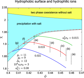
Figure 8: (Color online) Phase diagram of prewetting and precipitation transitions on a hydrophobic colloid with $a_{0}^{2}\gamma=0.08$. Three prewetting lines, corresponding to $a_{0}^{2}\sigma_{0}=0.015$, 0.018 and 0.021, are more extended than in the hydrophilic case in Fig.6. Precipitation on the colloid surface occurs above the broken red line. See Fig.9 for $\alpha$ and $\Gamma$ on vertical paths (a),$\dots$, and (g).

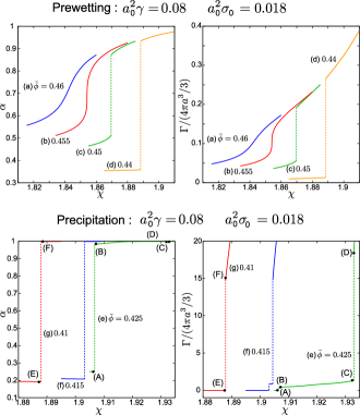
Figure 9: (Color online) Degree of ionization $\alpha$ (left) and normalized adsorption $\Gamma/(4\pi a^{3}/3)$ (right) vs $\chi$ on a hydrophobic colloid with $a_{0}^{2}\gamma=0.08$ and $a_{0}^{2}\sigma_{0}=0.018$ along paths (a) $\bar{\phi}=0.46$, (b) 0.455, (c) 0.45, (d) 0.44, (e) 0.425, (f) $0.415$, and (g) 0.41 (see their locations in Fig.8). Top: Behavior around the prewetting line at $a_{0}^{2}\sigma_{0}=0.018$ (middle line in Fig.8) along paths (a),(b), (c), and (d). Bottom: Large jumps across the precipitation line along the paths (e),(f), and (g) (dotted lines). On path (e), there is a prewetting transition between (A) and (B) and a precipitation transition between (C) and (D). Path (f) also passes the two transitions. Path (g) passes only the precipitation line.

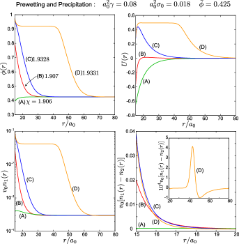
Figure 10: (Color online) $\phi(r)$ (left top), $U(r)$ (right top), $v_{0}n_{1}(r)$ on a semi-logarithmic scale (left bottom), and $v_{0}(n_{1}(r)-n_{2}(r))$ (right bottom) on a hydrophobic colloid at four points (A),(B), (C), and (D) on path (e) in Fig.9, where $a_{0}^{2}\gamma=0.08$, $a_{0}^{2}\sigma_{0}=0.018$, and $\bar{\phi}=0.425$. A prewetting transition occurs between (A) and (B), while a precipitation transition between (C) and (D). At (B), (C), and (D), the ions are enriched in the layer. In the inset in the right bottom plate, a small electric double layer is shown in the interface region around $r\cong 40a_{0}$ at (D).

The prewetting behavior is more exaggerated for a weakly hydrophobic surface under Eq.(2.29) than for a hydrophilic surface. In Subsec.IIC, we have discussed the changeover from a hydrophobic to hydrophilic surface with progress of ionization. Here, we examine the prewetting and precipitation transitions in the weakly hydrophobic case with $\gamma=0.08a_{0}^{-2}$ in Figs.8-17 and also in the strongly hydrophobic case with $\gamma=0.2a_{0}^{-2}$ in the lower plates in Fig.12.

In Fig.8, we display three examples of the prewetting line corresponding to $a^{2}\sigma_{0}=0.015$, 0.018, and 0.021, which are pushed downward with increasing $\sigma_{0}$. They even bend downward and much extend outside the bulk precipitation line. The precipitation line for a colloid (broken line) is inside the bulk precipitation region and is independent of $\sigma_{0}$ (as in Fig.6).

In Fig.9, we show the degree of ionization $\alpha$ and the excess adsorption $\Gamma$ defined in Eq.(5.2) as functions of $\chi$ for various $\bar{\phi}$. In the upper plates, the discontinuities across the prewetting line increase with increasing $\chi$, where the critical point is located at the smallest $\chi$ on the line. (In sharp contrast, they decrease with increasing $\chi$ in the hydrophilic case in Fig.6.) In the lower plates, $\alpha$ and $\Gamma$ are shown along paths, (e), (f), and (g), where (e) and (f) pass the prewetting and precipitation lines but path (g) passes the precipitation line only. In particular, on path (e), $\alpha$ changes from about 0.2 to values slightly smaller than unity across the prewetting line or between (A) and (B), while $\Gamma$ changes greatly across the precipitation line or between (C) and (D). The $\Gamma/(4\pi a^{3}/3)$ is $-0.0137$ at (A), 0.417 at (B), 1.30 at (C), and 19.1 at (D).

The jump of $\Gamma$ between (C) and (D) is very large and can be explained by minimization of $F_{\rm wet}$ in Eq.(4.15) jump .

In Fig.10, the profiles of $\phi(r)$, $U(r)$, $n_{1}(r)$, and $n_{1}(r)-n_{2}(r)$ are shown at points (A), (B), (C), and (D) on path (e) in the right bottom panel of Fig.9. At (A), which is below the prewetting line, the colloid surface is still hydrophobic with a negative surface value of $\phi^{\prime}=\partial\phi/\partial r$, $U(r)$ is negative, and the ions are weakly accumulated near the surface. At (B), which is slightly above the prewetting line, the surface is hydrophilic, $U$ has a small maximum, and the cations and the anions are both enriched near the surface. At (D) there is a thick wetting layer enriched with ions. In the right bottom panel, the charge accumulation near the surface and the electric double layer (in the inset) are shown, which are small because of small difference $g_{1}-g_{2}=2$ in this case. In passing, the value of $\chi$ at the precipitation transition is 1.9329, while it is $1.9320$ for $d=25a_{0}$ (not shown here). These values are only slightly larger than $\chi_{\rm p}=1.9246$.

V.4 Two colloids and their interaction free energy for hydrophobic surface and hydrophilic ions

Placing two hydrophobic colloids along the $z$ axis, we now calculate the profiles of $\phi$ and $U$ and the interaction free energy $F_{\rm int}(d)$ as a function of the distance $d$ between the two colloid centers in Figs.11-17. The profiles depend on $r=({x^{2}+y^{2}})^{1/2}$ and $z$. The degree of ionization $\alpha=\alpha(\theta)$ depends on the angle $\theta$ with respect to the $z$ axis. Its angle average is written as

$$\langle{\alpha}\rangle=\int_{0}^{\pi}d\theta\sin\theta~{}\alpha(\theta).$$ (5.3)

The precipitation transition is continuous for the present parameters, as stated at the beginning of this section.

V.4.1 Crossover from repulsive to attractive interaction

First, for $\bar{\phi}=0.425$, we examine the behavior around the prewetting transition with $a_{0}^{2}\gamma=0.08$ and $a_{0}^{2}\sigma_{0}=0.018$. In Fig.11, the left panel gives $F_{\rm int}$ vs $d$ for $\chi=1.88$ and 1.92. Remarkably, it is small and positive for $\chi=1.88$ but is negative and is much amplified for $\chi=1.92$. The right panel displays the corresponding $\phi(r,z)$ at $d=44a_{0}=2.93a$, where $(\Gamma/(4\pi a^{3}/3),\langle{\alpha}\rangle)=(-0.0198,0.305)$ for $\chi=1.88$ and $(1.30,0.941)$ for $\chi=1.92$ with a big difference in $\Gamma$. The screening length $\kappa^{-1}$ in Eq.(3.5) is $7.94a_{0}$, while the correlation length $\bar{\xi}$ in Eq.(3.11) is $2.71a_{0}$ for $\chi=1.88$ and $3.23a_{0}$ for $\chi=1.92$. The surface remains hydrophobic ($\phi^{\prime}>0$) for $\chi=1.88$ but becomes hydrophilic ($\phi^{\prime}<0$) for $\chi=1.92$.

On the other hand, at the critical composition $\bar{\phi}=0.5$, there is no prewetting transition, though the precipitation occurs for $\chi>\chi_{\rm p}=1.9675$, as can be seen in Fig.4. The instability point $\tau=\tau_{c}$ occurs at $\chi=1.97$ since $v_{0}\tau_{c}=0.06$ (see Eqs.(3.9) and (3.11)). Thus, at $\bar{\phi}=0.5$, the physical quantities change continuously with varying $\chi$ below $\chi_{\rm p}$. In Fig.12, we show $F_{\rm int}$ vs $d$ in the left and the corresponding $\phi(r,z)$ at $d=44a_{0}=2.93a$ in the right for $\bar{\phi}=0.5$. The screening length $\kappa^{-1}$ is $8.14a_{0}$, while the correlation length $\bar{\xi}$ is $1.14a_{0}$ for $\chi=1.2$ and $14.1a_{0}$ for $\chi=1.965$. (i) The upper panels are for the weakly hydrophobic case with $a_{0}^{2}\gamma=0.08$ and $a_{0}^{2}\sigma_{0}=0.018$, where $(\Gamma/(4\pi a^{3}/3),\langle{\alpha}\rangle)=(0.063,0.65)$ for $\chi=1.2$ and $(3.15,0.98)$ for $\chi=1.965$. The surface is weakly hydrophilic at $\chi=1.2$ and is strongly hydrophilic at $\chi=1.965$. (ii) The lower plates are for the strongly hydrophobic case with $a_{0}^{2}\gamma=0.2$ and $a_{0}^{2}\sigma_{0}=0.01$, where $(\Gamma/(4\pi a^{3}/3),\langle{\alpha}\rangle)=(-0.093,0.64)$ for $\chi=1.2$ and $(-1.31,0.32)$ for $\chi=1.965$. The adsorption of the oil component is enhanced on approaching the criticality.

In the weakly hydrophobic case in the upper plates in Fig.12, the linear theory fairly holds at $\chi=1.2$, while it breaks down at $\chi=1.965$. In fact, $F_{\rm int}(d)/k_{B}T$ at $d\cong 2a$ is 3.71 (linear theory) and 2.38 (nonlinear theory) for $\chi=1.2$, while it is -22.4 (linear theory) and -3.44 (nonlinear theory) for $\chi=1.965$. The surface value of $\psi=\phi-{\bar{\phi}}$ is about 0.02 for $\chi=1.2$ and 0.25 for $\chi=1.965$, while $U\sim-1$ both for these cases.

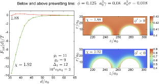
Figure 11: (Color online) Normalized interaction free energy $F_{\rm int}(d)/T$ vs normalized separation distance $d/a_{0}$ (left) and $\phi(r,z)$ at $d=44a_{0}=2.93a$ (right) for $\bar{\phi}=0.425$, where $a_{0}^{2}\gamma=0.08$, and $a_{0}^{2}\sigma_{0}=0.018$. The system is below a prewetting line at $\chi=1.88$ and above it at $\chi=1.92$, where $F_{\rm int}$ changes its sign from positive to negative. The surface is hydrophobic with $\phi^{\prime}={\mbox{\boldmath$\nu$}}\cdot\nabla\phi>0$ (see Eq.(2.24)) at $\chi=1.88$, but is hydrophilic with $\phi^{\prime}<0$ due to an increase in $\alpha$ at $\chi=1.92$. The color represents $\phi$ according to the color bar attached.

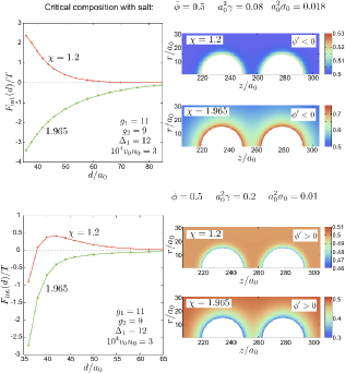
Figure 12: (Color online) Normalized interaction free energy $F_{\rm int}(d)/k_{B}T$ vs normalized separation distance $d/a_{0}$ (left) and $\phi(r,z)$ at $d=44a_{0}=2.93a$ (right) at the critical composition $\bar{\phi}=0.5$, where there is no prewetting transition. Top: Those for (originally) weakly hydrophobic surface with $a_{0}^{2}\gamma=0.08$ and $a_{0}^{2}\sigma_{0}=0.018$ at $\chi=1.2$ and $\chi=1.965$. Here $F_{\rm int}$ changes its sign on approaching the solvent criticality The surface becomes hydrophilic ($\phi^{\prime}<0$) weakly for $\chi=1.2$ and strongly for $\chi=1.965$ due to ionization. Bottom: Those for strongly hydrophobic surface with $a_{0}^{2}\gamma=0.2$ and $a_{0}^{2}\sigma_{0}=0.01$ at $\chi=1.2$ and $\chi=1.965$. Here the surface remains hydrophobic even for full ionization.

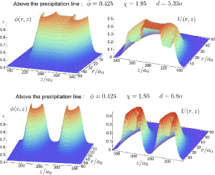
Figure 13: (Color online) $\phi(r,z)$ (left) and $U(r,z)$ (right) around two hydrophobic colloids above a precipitation line, where $a_{0}^{2}\gamma=0.08$, $a_{0}^{2}\sigma_{0}=0.018$, and $\bar{\phi}=0.425$. Wetting layers of two colloids are bridged at $d=5.33a=80a_{0}$ (top) and are disconnected for $6.8a=102a_{0}$ (bottom). The surface has become hydrophilic with $\phi^{\prime}<0$.

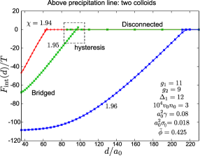
Figure 14: (Color online) Normalized interaction free energy $F_{\rm int}(d)/T$ as a function of normalized distance $d/a_{0}$ above a precipitation line, where $\chi=1.94$, $1.95$ and $1.96$ for three curves (from above). Wetting layers of two colloids are bridged for small $d$ but are disconnected for large $d$. There is hysteretic behavior between these two states (see Fig.15).

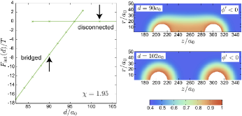
Figure 15: (Color online) Left: Normalized interaction free energy $F_{\rm int}(d)/T$, exhibiting hysteresis between bridged and disconnected states of wetting layers for $\chi=1.95$ in the box region in Fig.14. There can be a metastable state in an interval of $d$ (left). Composition $\phi(r,z)$ in wetting layers at the two states marked by the arrows in the left.

V.4.2 Bridged and disconnected wetting layers

Next, we examine the wetting layer behavior after the precipitation transition in Figs.13-15 for $\bar{\phi}=0.425$. In Fig.13, the profiles of $\phi(r,z)$ and $U(r,z)$ are presented above the precipitation line with the same parameter values as in Fig.11. Here we have thick wetting layers on the two colloids and they are bridged for $d=80a_{0}=5.33a$ (top plates) and are disconnected for $102a_{0}=6.8a$ (bottom plates). In Fig.14, the interaction free energy $F_{\rm int}(d)$ is shown as a function of $d$, where the three curves correspond to $\chi=1.94$, $1.95$, and $1.96$. At relatively short separation $d=44a_{0}$, for instance, $\Gamma$ increases with increasing $\chi$ as $\Gamma/(4\pi a^{3}/3)=3.87$, $7.20$, and $23.3$, respectively. We recognize that the wetting layers are bridged for relatively small $d$ but are disconnected for large $d$, exhibiting hysteresis. The $F_{\rm int}(d)/T$ assumes negative values of order $-100$ while bridged, but it becomes very small once detached. For larger colloid radii, the value of $F_{\rm int}(d)/T$ should be much more amplified ($\propto a^{3})$. In Fig.15, the hysteretic transition behavior is illustrated between the bridged and disconnected sates. That is, in an interval of $d$, we find two linearly stable profiles, where one is metastable with a higher $F_{\rm int}(d)$.

It is worth noting that Hopkins et al. Evans also found a bridging of adsorption layers of two approaching neutral colloid particles in a mixture solvent close to the coexistence curve.

V.4.3 Partial wetting on hydrophobic surface

In the previous examples of hydrophobic colloids, the surface is in a completely wetted state above the precipitation line in the composition range ${\bar{\phi}}=0.4-0.5$. However, for smaller ${\bar{\phi}}$, a hydrophobic colloid surface can be partially wetted if $\gamma$ is not very large.

In Fig.16, at $\bar{\phi}=0.3$, we display such composition profiles $\phi(r,z)$ around two hydrophobic colloids at $d=44a_{0}=2.93a$ by changing $\chi$. The other parameters are common to those in Figs.11 and 13. For $\chi>\chi_{\rm p}=1.12$, there appears a water-rich region partially wetting the colloid surface. The surface is partially wetted for $\chi=1.25$, 1.55, and $1.85$, but is completely covered by the water-like component at $\chi=2$. Here, $\alpha$ in the non-wetted regions is 0.082, 0.058, and 0.051 for $\chi=1.85$, 1.55, and 1.25, respectively, while $\alpha$ is nearly equal to unity in the wetted surface regions. In these examples, the number of the counterions from the wetted surface is only about $0.4\%$ of the number of the cations in the wetting water-rich region, where the latter is about $5600$ for $\chi=1.25$.

In Fig.17, we vary $d$ at $\bar{\phi}=0.3$ and $\chi=1.55$ to see how the partial wetting of two hydrophobic colloids is changed between bridged and disconnected states. In the left panel, $F_{\rm int}(d)$ is displayed as a function of $d$, where hysteresis is exhibited between these two states. In the right panel, we show $\phi(r,z)$ in the connected case at $d=60a_{0}$ and in the disconnected case at at $d=72a_{0}$. In the latter case, a water-rich droplet is partially wetting the left colloid. In these cases, $\alpha$ is 0.99 in the wetted part and about 0.05 in the nonwetted part.

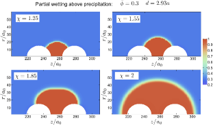
Figure 16: (Color online) Partially or completely wetting profiles of $\phi(r,z)$ around two hydrophobic colloids for $\bar{\phi}=0.3$ with $d=44a_{0}=2.93a$, where $\chi=1.25$, 1.55, 1.85, and 2 above the bulk precipitation value $\chi_{\rm p}=1.12$, The other parameters are common to those in Figs.11 and 13-15.

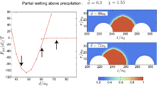
Figure 17: (Color online) Two partially wetted, hydrophobic colloids in a bridged or disconnected state for $\bar{\phi}=0.3$ at $\chi=1.55$. The other parameters are common to those in Fig.16. Left: $F_{\rm int}(d)/k_{B}T$ vs $d/a_{0}$ with hysteresis between the two states. Arrows indicate $d/a_{0}=44$, 60, 72. Right: $\phi(r,z)$ at $d/a_{0}=60$ (bridged) and 72 (disconnected). Profile at $d/a_{0}=44$ is in the top right panel in Fig.16.

V.5 Antagonistic ions

With antagonistic ions added, oscillatory response can arise against local disturbances even if the system is in a homogeneous state in the bulk region, as has been discussed in the linear theory in Sec.III. Here, we set $g_{1}=-g_{2}=13$, $a_{0}^{2}\gamma=0.2$, $a_{0}^{2}\sigma=0.016$, and $\bar{\phi}=0.5$.

In Fig.18, we show $\phi(r)$ and $U(r)$ as functions of $r/a_{0}$ around a single colloid, where three curves correspond to $\chi=1.961$, $1.965$, and $1.966$. Oscillatory behavior is amplified with increasing $\chi$. The system tends to a homogeneous state far from the colloid for the smaller two $\chi$, but it is in a periodically modulated phase for the largest $\chi$, since the homogeneous state is linearly unstable for $\chi>1.9651$. In Fig.19, we examine the case of two colloids, In its left panel, the interaction free energy $F_{\rm int}$ is plotted as a function of $d$ for two colloids for $\chi=1.95$, $1.961$ and $1.965$. In its right panel, the profile of $\phi(r,z)$ is given for $\chi=1.965$ at $d=49a_{0}=3.27a$, where a homogeneous state is linearly stable.

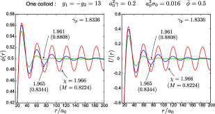
Figure 18: (Color online) $\phi(r)$ and $U(r)$ around a hydrophobic colloid for antagonistic salt with $g_{1}=-g_{2}=13$, where $a_{0}^{2}\gamma=0.2$, $a_{0}^{2}\sigma_{0}=0.016$, and $\bar{\phi}=0.5$. Three curves correspond to $\chi=1.961$ (green), $1.965$ (blue) and $1.966$ (red) Parameter $M$ in Eq.(3.21) in the linear theory is equal to 0.8808, 0.8344, 0.8224, respectively. Oscillatory behavior is amplified with increasing $\chi$. The system tends to be homogeneous far from the colloid for the first two curves, while a mesophase is realized for the third curve.

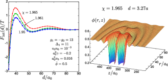
Figure 19: (Color online) Left: Normalized interaction free energy $F_{\rm int}/k_{B}T$ as a function of $d$ for two colloids with antagonistic ions, where $a_{0}^{2}\gamma=0.2>0$, $a_{0}^{2}\sigma_{0}=0.016$, and $\bar{\phi}=0.5$. Three curves correspond to $\chi=1.950$, $1.961$ and $1.965$ from below. Instability occurs at $\chi>1.9651$, so homogeneity is attained far from the colloids. Right: $\phi(r,z)$ around two hydrophobic colloids at $d=49a_{0}=3.27a$ for $\chi=1.965$.

VI Summary and remarks

In summary, we have examined how ionizable colloids influence the ion distributions and the composition field in binary polar solvents. These perturbations then give rise to the interaction free energy $F_{\rm int}(d)$ between two colloids as a function of the distance $d$ between their centers. We summarize our main results.
(i) In Sec.II, we have introduced a Ginzburg-Landau model in the presence of negatively ionizable colloids. The fundamental fluctuating variables are the composition $\phi$, the ion densities $n_{i}$, and the degree of ionization $\alpha$, which are inseparably coupled in the presence of the selective solvation. Important parameters in the bulk free energy are the interaction parameter $\chi$ (determined by the temperature $T$), the average composition $\bar{\phi}$, the average anion density $n_{0}$, and the solvation parameters $g_{i}$. Those related to the colloid are the radius $a$, the molecular interaction parameter $\gamma$ representing the surface field, the density of the ionizable groups on the surface $\sigma_{0}$, and the composition-dependent ionization free energy $T(\Delta_{0}-\Delta_{1}\phi)$, which appear in the boundary condition (2.24) on $\phi$ and the mass action law (2.26) for $\alpha$.
(ii) In Sec.III, we have presented a linear theory of the electrostatic and compositional disturbances produced by charged colloids, which is a generalization of the Debye-H$\ddot{\rm u}$ckel and DLVO theories. In the linear scheme, the colloid interaction free energy $F_{\rm int}(d)$ is a linear combinations of two Yukawa functions $e^{-q_{i}(d-2a)}/(1+q_{i}/a)^{2}d$ as a function of the colloid separation distance $d$ in terms of two characteristic wave numbers $q_{i}$. In the weak coupling linit $g_{a}=g_{1}-g_{2}\to 0$, they tend to the DLVO interaction in Eq.(1.2) and the adsorption-induced attraction in Eq.(1.5).
(iii) In Sec.IV, we have presented a theory of precipitation on the colloid surface assuming a completely wetting layer, which is induced by the selective solvation of hydrophilic ions far from the solvent coexistence curve. This precipitation occurs at small $\chi$ for relatively small $\bar{\phi}$ (say, 0.1) (see the left panel of Fig.4). However, the growth of the layer thickness is slow with increasing $\chi$ for small $\bar{\phi}$. For ${\bar{\phi}}\gtrsim\phi_{c}$ precipitation occurs close to the solvent coexistence curve.
(iv) In Sec.V, we have presented numerical results on precipitation and prewetting on the colloid surface for hydrophilic $(\gamma<0$) and hydrophobic $(\gamma>0$) surfaces in the nonlinear theory. We are particularly interested in the weakly hydrophobic surface satisfying Eq.(2.29). Such a surface is hydrophobic without ionization, but becomes hydrophilic with progress of ionization. Also the prewetting phase transition is more dramatic for such a hydrophobic surface than for a hydrophilic surface as in Figs.6 and 8. Wetting layer formation occurs above a precipitation line, which weakly depends on the radius $a$ and is located slightly above the bulk precipitation line $\chi=\chi_{\rm p}$. Such layers undergo a bridging transition with a great change in the interaction free energy $F_{\rm int}$ as in Figs.13-15. They either completely or partially wet the surface depending on the average composition $\bar{\phi}$ as in Figs.16-18. For antagonistic ion pairs, oscillation can be seen the composition and potential profiles as a function of the separation distance $d$ as in Fig.18, but it is largely masked in $F_{\rm int}$ in Fig.19.

We make some remarks.
1) Our coarse-grained theory is inaccurate on the angstrom scale, but the solvation parameters $g_{i}$ and the ionization parameter $\Delta_{1}$ can be made very large, so the precipitation and prewetting transitions on the colloid surface have been predicted. We also note that the molecular volumes of the two components are often very different in real mixtures. For example, those of D₂O and tri-methylpyridine (the inverse densities of the pure components) are 28 and 168 ų, respectively Sadakane . The coefficient $C$ in Eq.(2.1) of the gradient free energy remains an arbitrary constant comment-gra , though we have set $C=2a_{0}^{-1}$ in Sec.V.
2) We believe that the previous observations of colloid aggregation Beysens ; Maher ; Kaler ; Guo ; Bonn should be induced by overlapping of enhanced adsorption or wetting layers on the colloid surface Evans . If the ions are neglected, colloid particles constitue a selective solute added in a binary mixture Kaler . Furthermore, if the selectivity is high, our previous theory Okamoto indicates a solute-induced phase separation with a phase diagram as in Fig.4. This aspect should be studied in more detail.
3) Wetting behavior remains unexplored in the presence of a highly selective solute. It becomes even more complex if the substrate itself is ionizable. We have realized both complete and partial wetting on ionizable colloid surfaces, but the information gained is still fragmentary because many parameters are involved in the problem.
4) The effects of the critical fluctuations on the interactions between solid surfaces are very intriguing Fisher ; Krech ; JSP ; Nature2008 . Ions should further promote bridging of highly adsorbing or wetting layers.
5) For antagonistic ion pairs, the oscillatory behavior in the colloid interaction in Fig.19 is rather mild, though it is evident in the composition and potential profiles. It becomes more evident in the interaction between two parallel plates, as in the case of liquid crystals Uchida .
6) For polyelectrolytes including ionized gels, there are a number of unsolved problems arising from selective solvation. Even in one-component solvents, ions interact differently with polymer segments and solvent molecules Onuki-Okamoto . In mixture solvents (water-alcohol), a wetting film should be formed around a chain, as stated in Sec.I Onuki-Okamoto ; B1 ; B2 ; B3 . The Manning-Oosawa counterion condensation mechanism should be modified for mixture solvents.

Appendix A: Pair correlation functions

VI.0.1 Composition fluctuations

We examine the structure factor of the composition fluctuations $S(q)={\langle{|\phi_{\small{\mbox{\boldmath$q$}}}|^{2}}\rangle}_{\rm e}$, where $\phi_{\small{\mbox{\boldmath$q$}}}$ is the Fourier component of $\phi({\mbox{\boldmath$r$}})$ with wave vector $q$ and $\langle{\cdots}\rangle_{\rm e}$ denotes taking the thermal average. The mean-field structure factor reads Onuki-Kitamura ; OnukiPRE ,

$$\frac{1}{S(q)}=\tau-\tau_{c}+C{q^{2}}\bigg{[}1-\frac{\gamma_{\rm p}^{2}\kappa^{2}}{q^{2}+\kappa^{2}}\bigg{]},$$ (A1)

in terms of $\tau$ in Eq.(3.6), $\tau_{c}$ in Eq.(3.9), and $\gamma_{\rm p}$ in Eq.(3.22). If the right hand side of Eq.(A1) is expanded with respect to $q^{2}$, the coefficient in front of $q^{2}$ is $C(1-\gamma_{\rm p}^{2})$. Thus a Lifshitz point is realized at $\gamma_{\rm p}=1$. (i) For $\gamma_{\rm p}<1$, $S(q)$ is maximum at $q=0$ and $S(q)^{-1}\propto\bar{\xi}^{-2}+(1-\gamma_{\rm p}^{2})q^{2}$ for $q\ll\kappa$, so a thermodynamic instability occurs for $\tau<\tau_{c}$ at long wavelengths. To be precise, $\tau_{c}$ is the shift in this case. (ii) For $\gamma_{\rm p}>1$, $S(q)$ has a peak at

$$q_{\rm m}=(\gamma_{\rm p}-1)^{1/2}\kappa.$$ (A2)

The corresponding peak height is given by

$$S(q_{\rm m})=C^{-1}\kappa^{-2}/[M^{2}-(\gamma_{\rm p}-1)^{2}].$$ (A3)

which diverges as $\gamma_{\rm p}-1\to M=(\kappa\bar{\xi})^{-1}$. A mesophase (a charge-density-wave phase) should emerge for $\gamma_{\rm p}-1>M$, as was observed experimentally Sadakane .

Furthermore, from Eq.(A1), the quadratic equation (3.19) is identical to $S(q)^{-1}=0$ with $q^{2}=-\kappa^{2}\lambda$. In terms of $q_{1}$ and $q_{2}$ in Eq.(3.18), we obtain

$$CS(q)=\frac{q^{2}+\kappa^{2}}{(q^{2}+q_{1}^{2})(q^{2}+q_{2}^{2})}.$$ (A4)

The inverse Fourier transformation of $S(q)$ yields the pair correlation $g(r)=\langle{\delta\phi({\mbox{\boldmath$r$}})\delta\phi({\mbox{\boldmath$0$}})}\rangle_{\rm e}$ for the composition fluctuations. It follows a sum of the two Yukawa functions,

$$g(r)=\frac{(\lambda_{1}-1)e^{-q_{1}r}-(\lambda_{2}-1)e^{-q_{2}r}}{4\pi C(\lambda_{1}-\lambda_{2})r}.$$ (A5)

In particular, in the region $|M-1|<\gamma_{\rm p}<M+1$, $q_{1}$ and $q_{2}$ are complex conjugates and $g(r)$ behaves as

$$g(r)=\frac{e^{-q_{R}r}}{4\pi Cr}\bigg{[}\cos(q_{I}r)+({q_{a}^{2}-q_{I}^{2}-\kappa^{2}})\frac{\sin(q_{I}r)}{2q_{R}q_{I}}\bigg{]},$$ (A6)

where $q_{R}$ and $q_{I}$ are are given in Eq.(3.24).

VI.0.2 Ion fluctuations

We eliminate the composition fluctuations assuming their Gaussian distribution, where the ion densities are held fixed. The resultant ion-ion potentials read Onuki-Kitamura ; OnukiPRE

$${V_{ij}(r)}=Z_{i}Z_{j}\frac{e^{2}}{\varepsilon r}-\frac{Tg_{i}g_{j}}{4\pi C}\frac{1}{r}{e^{-r/\xi}},$$ (A7)

where $Z_{1}$ and $Z_{2}$ are $\pm 1$ in the monovalent case. The second term is the composition-induced interaction decaying exponentially with the correlation length $\xi=(C/{\tau})^{1/2}$. It is attractive among the ions of the same species $(i=j)$. It dominates over the Coulomb repulsion for $g_{i}^{2}>4\pi C\ell_{B}$ in the range $r\lesssim\xi$, under which there should be a tendency of ion aggregation. In the antagonistic case ($g_{1}g_{2}<0$), the cations and anions repel one another for $|g_{1}g_{2}|>4\pi C\ell_{B}$ in the range $r\lesssim\xi$, leading to charge-density-wave formation near the criticality. Note that the shifted correlation length $\bar{\xi}$ in Eq.(3.11) has appeared in the colloid-colloid interaction, where both the composition and ion densities are eliminated.

In our recent review papers Current ; Nara , we have furthermore calculated the structure factors among the ion densities $G_{ij}(q)={\langle{n_{i\small{\mbox{\boldmath$q$}}}n_{j\small{\mbox{\boldmath$q$}}}^{*}}\rangle}_{\rm e}/n_{0}$. Further using Eq.(A4) we find

$${G_{11}(q)}=1-\frac{1/2}{u+1}+\frac{\gamma_{\rm p}^{2}[u+w(u+1)]^{2}/2}{(u+1)(u+\lambda_{1})(u+\lambda_{2})},$$

$${G_{12}(q)}=\frac{1/2}{u+1}+\frac{\gamma_{\rm p}^{2}[w^{2}(u+1)^{2}-u^{2}]/2}{(u+1)(u+\lambda_{1})(u+\lambda_{2})},$$ (A8)

where $u=q^{2}/\kappa^{2}$ and $w=(g_{1}+g_{2})/(g_{1}-g_{2})$. The $G_{22}(q)$ is obtained if $w$ in $G_{11}(q)$ is replaced $-w$. The inverse Fourier transformation of these structure factors gives rise to the pair correlation functions $g_{ij}(r)=\langle{\delta n_{i}({\mbox{\boldmath$r$}})\delta n_{j}({\mbox{\boldmath$0$}})}\rangle_{\rm e}/n_{0}$. We notice that the terms proportional to $e^{-\kappa r}/r$ cancel to vanish from the relation $(1-\lambda_{1})(1-\lambda_{2})=\gamma_{\rm p}^{2}$. Thus,

$$g_{ij}(r)={\delta({\mbox{\boldmath$r$}})}\delta_{ij}-(K_{1}^{ij}{e^{-q_{1}r}}+K_{2}^{ij}{e^{-q_{2}r}})\frac{1}{r},$$ (A9)

where the $\delta$ function appears due to the self correlation and $K_{1}^{ij}$ and $K_{2}^{ij}$ are appropriately defined constants.

Appendix B: Calculations in the linear theory for one and two colloid particles

First, we seek the fundamental profiles $U_{0}(r)$ and $\psi_{0}(r)$ around a single colloid particle induced by by the boundary conditions (3.12) and 83.13), where the surface charge is fixed. They depend only on the distance $r$ from the colloid center. For $r>a$ we may set

$$U_{0}(r)=g_{a}(\alpha_{1}{e^{-q_{1}r}}-\alpha_{2}{e^{-q_{2}r}})/{r},$$ (B1)

$$\psi_{0}(r)=(\beta_{1}e^{-q_{1}r}-\beta_{2}{e^{-q_{2}r}})/{r}.$$ (B2)

For $r<a$, we have $U_{0}(r)=U_{0}(a)=$const. from $\nabla^{2}U_{0}=0$. From Eqs.(3.7), (3.8), and (3.21), we obtain

$$\beta_{i}=(1-\lambda_{i})\alpha_{i},$$ (B3)

$$[\lambda_{i}-M^{2}+\gamma_{\rm p}^{2}]\beta_{i}=\gamma_{\rm p}^{2}\alpha_{i},$$ (B4)

which hold for $i=1,2$. The boundary conditions (3.12) and (3.13) give

$$\alpha_{1}^{\prime}-\alpha_{2}^{\prime}=-4\pi\ell_{B}{\bar{\sigma}}/g_{a},$$ (B5)

$$\alpha_{1}^{\prime}(1-\lambda_{1})-\alpha_{2}^{\prime}(1-\lambda_{2})=-{\bar{\gamma}}/C,$$ (B6)

where $\alpha_{i}^{\prime}=\alpha_{i}(1+q_{i}a)e^{-q_{i}a}/a^{2}$. Using the relation $(\lambda_{1}-1)(\lambda_{2}-1)=\gamma_{\rm p}^{2}$, we solve these equations to obtain

$$\alpha_{i}=\frac{e^{q_{i}a}B_{i}(\lambda_{1}-\lambda_{2})}{({1+q_{i}a})(1-\lambda_{i})},$$ (B7)

where $B_{1}$ and $B_{2}$ are defined in Eq.(3.26). We thus confirm Eqs.(3.25) and (3.26). In this one-colloid case $\Delta\Omega$ in Eq.(3.17) is written as ${F_{\rm self}}$. Some calculations give

$${F_{\rm self}}={2\pi a^{3}T}\bigg{[}\frac{E_{1}}{1+q_{1}a}-\frac{E_{2}}{1+q_{2}a}\bigg{]},$$ (B8)

where $E_{1}$ and $E_{2}$ are defined in Eq.(3.31).

Next we consider two colloid particles at positions ${\mbox{\boldmath$r$}}_{1}$ and ${\mbox{\boldmath$r$}}_{2}$ separated by $d=|{\mbox{\boldmath$r$}}_{1}-{\mbox{\boldmath$r$}}_{2}|>2a$ under the condition of fixed surface charge. In the colloid exterior ($|{\mbox{\boldmath$r$}}-{\mbox{\boldmath$r$}}_{1}|>a$ and $|{\mbox{\boldmath$r$}}-{\mbox{\boldmath$r$}}_{2}|>a$), $U$ and $\psi$ are expressed as

$$U=U_{0}(|{\mbox{\boldmath$r$}}-{\mbox{\boldmath$r$}}_{1}|)+U_{0}(|{\mbox{\boldmath$r$}}-{\mbox{\boldmath$r$}}_{2}|)+W({\mbox{\boldmath$r$}}),$$ (B9)

$$\psi=\psi_{0}(|{\mbox{\boldmath$r$}}-{\mbox{\boldmath$r$}}_{1}|)+\psi_{0}(|{\mbox{\boldmath$r$}}-{\mbox{\boldmath$r$}}_{2}|)+\Psi({\mbox{\boldmath$r$}}),$$ (B10)

where $U_{0}$ and $\psi_{0}$ are the fundamental profiles for a single colloid. In the colloid exterior, we expand the corrections $W$ and $\Psi$ around the center of the first colloid at ${\mbox{\boldmath$r$}}_{1}$ as

$$W=g_{a}\sum_{i,\ell}a_{i\ell}k_{\ell}(q_{i}|{\mbox{\boldmath$r$}}-{\mbox{\boldmath$r$}}_{1}|)P_{\ell}(\theta_{1}),$$ (B11)

$$\Psi=\sum_{i,\ell}(1-\lambda_{i})a_{i\ell}k_{\ell}(q_{i}|{\mbox{\boldmath$r$}}-{\mbox{\boldmath$r$}}_{1}|)P_{\ell}(\theta_{1}),$$ (B12)

where $a_{i\ell}$ ($i=1,2$ and $\ell=0,1,\cdots)$ are unknown coefficients to be determined below. The $P_{\ell}(\theta_{1})$ are the spherical harmonic functions with $\theta_{1}$ being the angle between ${\mbox{\boldmath$r$}}-{\mbox{\boldmath$r$}}_{1}$ and ${\mbox{\boldmath$r$}}_{2}-{\mbox{\boldmath$r$}}_{1}$. We introduce the modified spherical Bessel functions $i_{\ell}(x)$ and $k_{\ell}(x)$ Watson . They satisfy $i_{\ell}^{\prime\prime}+2i_{\ell}^{\prime}/x-\ell(\ell+1)i_{\ell}/x^{2}=i_{\ell}$ and $k_{\ell}^{\prime\prime}+2k_{\ell}^{\prime}/x-\ell(\ell+1)k_{\ell}/x^{2}=k_{\ell}$, where we write $i_{\ell}^{\prime}=di_{\ell}/dx$, $k_{\ell}^{\prime}=dk_{\ell}/dx$, $i_{\ell}^{\prime\prime}=d^{2}i_{\ell}/dx^{2}$, and $k_{\ell}^{\prime\prime}=d^{2}k_{\ell}/dx^{2}$. We have $i_{\ell}\sim x^{\ell}$ as $x\to 0$ and $k_{\ell}\sim e^{-x}$ as $x\to\infty$. In particular Bessel ,

$$i_{0}(x)=\sinh x/x,\quad k_{0}(x)=e^{-x}/x.$$ (B13)

Thus, $i_{\ell}P_{\ell}$ and $k_{\ell}P_{\ell}$ satisfy the Helmholtz equations,

$$(\nabla^{2}-q_{i}^{2})[i_{\ell}(q_{i}|{\mbox{\boldmath$r$}}-{\mbox{\boldmath$r$}}_{1}|)P_{\ell}(\theta_{1})]=0,$$

$$(\nabla^{2}-q_{i}^{2})[k_{\ell}(q_{i}|{\mbox{\boldmath$r$}}-{\mbox{\boldmath$r$}}_{1}|)P_{\ell}(\theta_{1})]=0.$$ (B14)

With these relations and Eq.(3.7), we derive Eq.(B12) from Eq.(B11). In Eqs.(B9) and (B10) we also need to expand $U_{0}(|{\mbox{\boldmath$r$}}-{\mbox{\boldmath$r$}}_{2}|)$ and $\psi_{0}(|{\mbox{\boldmath$r$}}-{\mbox{\boldmath$r$}}_{2}|)$ around ${\mbox{\boldmath$r$}}_{1}$ in terms of $P_{\ell}(\theta_{1})$. To this end, we use the following mathematical relation Ohshima ; Watson ,

$$\frac{e^{-q|{\mbox{\boldmath$r$}}-{\mbox{\boldmath$r$}}_{2}|}}{|{\mbox{\boldmath$r$}}-{\mbox{\boldmath$r$}}_{2}|}=\sum_{\ell}(2\ell+1)qk_{\ell}(qd)i_{\ell}(q|{\mbox{\boldmath$r$}}-{\mbox{\boldmath$r$}}_{1}|)P_{\ell}(\theta_{1}),$$ (B15)

which holds for Re$(q)>0$ and in the region $|{\mbox{\boldmath$r$}}-{\mbox{\boldmath$r$}}_{1}|<d=|{\mbox{\boldmath$r$}}_{1}-{\mbox{\boldmath$r$}}_{2}|$. On the other hand, in the interior of the first colloid $|{\mbox{\boldmath$r$}}-{\mbox{\boldmath$r$}}_{1}|<a$, we have $\nabla^{2}U=0$ so that we may assume the expansion,

$$U=U_{0}(a)+g_{a}\sum_{\ell}b_{\ell}|{\mbox{\boldmath$r$}}-{\mbox{\boldmath$r$}}_{1}|^{\ell}P_{\ell}(\theta_{1}).$$ (B16)

We can calculate the coefficients $a_{i\ell}$ and $b_{\ell}$ from the boundary conditions (3.12) and (3.13) and the continuity of $U$ at the colloid surface. We are interested in the free energy deviation $\Delta\Omega$ in Eq.(3.17). For two symmetric colloids, we obtain

$${\Delta\Omega}/T=4\pi a^{2}[{\bar{\sigma}}\langle{\psi}\rangle_{0}-\bar{\gamma}\langle{U}\rangle_{0}],$$ (B17)

where $\langle{\cdots}\rangle_{0}$ denotes taking the surface average on the colloid 1 ($=\int_{0}^{\pi}d\theta_{1}\sin\theta_{1}(\cdots)/2$ at $|{\mbox{\boldmath$r$}}-{\mbox{\boldmath$r$}}_{1}|=a$). Thus $\Delta\Omega$ arises from the terms with $\ell=0$ in Eqs.(B11), (B12), and (B15). For $\ell=0$, the boundary conditions (3.12) and (3.13) simply yield

$$\sum_{i}q_{i}[\alpha_{i0}q_{i}k_{0}(q_{i}d)i_{i0}^{\prime}+a_{i0}k_{i0}^{\prime}]=0,$$ (B18)

$$\sum_{i}(1-\lambda_{i})q_{i}[\alpha_{i0}q_{i}k_{0}(q_{i}d)i_{i0}^{\prime}+a_{i0}k_{i0}^{\prime}]=0.$$ (B19)

For simplicity, we write $i_{0}(q_{i}a)$, $i_{0}^{\prime}(q_{i}a)$, $k_{0}(q_{i}a)$, and $k_{0}^{\prime}(q_{i}a)$ as $i_{i0}$, $i_{i0}^{\prime}$, $k_{i0}$, and $k_{i0}^{\prime}$, respectively, suppressing $q_{i}a$. In Eq.(B18) there is no contribution from the electric field within the colloid ($\propto\varepsilon_{\rm p}$). This is because the angle average of $({\mbox{\boldmath$r$}}-{\mbox{\boldmath$r$}}_{1})\cdot\mbox{\boldmath$E$}$ vanishes from Eq.(B16). For each $i$, it follows the relation,

$$a_{i0}=-\alpha_{i}q_{i}k_{0}(q_{i}d)i_{i0}^{\prime}/k_{i0}^{\prime}.$$ (B20)

Elimination of $a_{i0}$ yields

$${\langle{U}\rangle_{0}}=U_{0}(a)+g_{a}\sum_{i}\alpha_{i}k_{0}(q_{i}d)[i_{i0}-k_{i0}i_{i0}^{\prime}/k_{i0}^{\prime}].$$ (B21)

The expression for ${\langle{\psi}\rangle_{0}}$ also follows in the same manner. Further, using the relation,

$$i_{0}(x)-i_{0}^{\prime}(x)k_{0}(x)/k_{0}^{\prime}(x)=e^{x}/(1+x),$$ (B22)

we obtain simple Yukawa forms,

$${\langle{U}\rangle_{0}}=U_{0}(a)+g_{a}\sum_{i}\alpha_{i}\frac{e^{-q_{i}(d-a)}}{(1+q_{i}a)d},$$ (B23)

$${\langle{\psi}\rangle}_{0}=\psi_{0}(a)+\sum_{i}\alpha_{i}\frac{(1-\lambda_{i})e^{-q_{i}(d-a)}}{(1+q_{i}a)d}.$$ (B24)

We also have $b_{0}=[\langle{U}\rangle_{0}-U_{0}(a)]/g_{a}$ from the continuity of $U$. Substitution of Eqs.(B23) and (B24) into Eq.(B17) leads to the interaction free energy

$$F_{\rm int}=\Delta\Omega-2F_{\rm self},$$ (B25)

given in Eq.(3.30).

Finally, we calculate the terms with $\ell\geq 1$, though they do not contribute to $\Delta\Omega$ in the linear theory. From Eqs.(3.12) and (3.13) we express $a_{i\ell}$ in terms of $b_{\ell}$ and $\alpha_{i}$ as

$$a_{i\ell}=[\ell b_{\ell}a^{\ell-1}\mu_{i}\varepsilon_{\rm p}/\bar{\varepsilon}-\alpha_{i}q_{i}^{2}k_{\ell}(q_{i}d)i_{i\ell}^{\prime}]/q_{i}k_{i\ell}^{\prime},$$ (B26)

where $\mu_{1}=(1-\lambda_{2})/(\lambda_{1}-\lambda_{2})$ and $\mu_{2}=(1-\lambda_{1})/(\lambda_{2}-\lambda_{1})$ in the first term. We write $i_{i\ell}=i_{\ell}(q_{i}a)$, $i^{\prime}_{i\ell}=i_{\ell}^{\prime}(q_{i}a)$, $k_{i\ell}=k_{\ell}(q_{i}a)$, and $k^{\prime}_{i\ell}=k_{\ell}^{\prime}(q_{i}a)$. Requiring the continuity of the potential, we determine $b_{\ell}$ in the form,

$$b_{\ell}a^{\ell-1}=\frac{\sum_{i}\alpha_{i}q_{i}k_{\ell}(q_{i}d)\eta_{i\ell}}{a-\ell(\varepsilon_{\rm p}/\bar{\varepsilon})\sum_{i}\mu_{i}w_{i\ell}/q_{i}},$$ (B27)

where $\eta_{i\ell}=i_{i\ell}-i_{i\ell}^{\prime}k_{i\ell}/k_{i\ell}^{\prime}$ and $w_{i\ell}=k_{i\ell}/k_{i\ell}^{\prime}$. The term proportional to $\varepsilon_{\rm p}/\bar{\varepsilon}$ in the denominator in the right hand side arises from the boundary condition (3.12).

References

- (1) B.V. Derjaguin and L.D. Landau, Acta Physicochim.(USSR), 14, 633 (1941).
- (2) E.J.W. Verwey and J.Th.G. Overbeek, Theory of the Stability of Lyophobic Colloids (Elsevier, Amsterdam, 1948).
- (3) W. B. Russel, D. A. Saville, and W. R. Schowalter, Colloidal Dispersions (Cambridge University Press, Cambridge, 1989).
- (4) Y. Levin, Rep. Prog. Phys. 65, (2002) 1577.
- (5) , H. Ohshima, Theory of Colloid and Interfacial Electric Phenomena, (Academic Press, Amsterdam, 2004).
- (6) D. Beysens and D. Estve, Phys. Rev. Lett. 54, 2123 (1985); B.M. Law, J.-M. Petit, and D. Beysens, Phys. Rev. E, 57, 5782(1998); J.-M. Petit, B. M. Law, and D. Beysens, J.Colloid Interface Sci, 202, 441 (1998); D. Beysens and T. Narayanan, J. Stat. Phys. 95, 997 (1999).
- (7) P. D. Gallagher and J. V. Maher, Phys. Rev. A 46, 2012 (1992); P. D. Gallagher, M. L. Kurnaz, and J. V. Maher, Phys. Rev. A 46, 7750 (1992).
- (8) Y. Jayalakshmi and E. W. Kaler, Phys. Rev. Lett. 78, 1379 (1997).
- (9) H. Guo, T. Narayanan, M. Sztucki, P. Schall and G. Wegdam, Phys. Rev. Lett. 100, 188303 (2008)
- (10) D. Bonn, J. Otwinowski, S. Sacanna, H. Guo, G. Wegdam and P. Schall, Phys. Rev. Lett. 103, 156101 (2009).
- (11) J.L. Barrat and J.F. Joanny, Adv. Chem. Phys. XCIV, I. Prigogine, S.A. Rice Eds., John Wiley Sons, New York 1996.
- (12) C. Holm, J. F. Joanny, K. Kremer, R. R. Netz, P. Reineker, C. Seidel, T. A. Vilgis, and R. G. Winkler, Adv. Polym. Sci. 166, 67 (2004).
- (13) A.V. Dobrynin and M. Rubinstein, Prog. Polym. Sci. 30, 1049 (2005).
- (14) P. Hopkins, A.J. Archer, and R. Evans, J. Chem. Phys. 131, 124704 (2009).
- (15) J. N. Israelachvili, Intermolecular and Surface Forces (Academic Press, London, 1991).
- (16) A. Onuki and H. Kitamura, J. Chem. Phys. 121, 3143 (2004).
- (17) A. Onuki, Phys. Rev. E 73, 021506 (2006); J. Chem. Phys. 128, 224704 (2008).
- (18) T. Araki and A. Onuki, J. Phys.: Condens. Matter 21, 424116 (2009); A. Onuki, T. Araki, and R. Okamoto, J. Phys.: Condens. Matt. 23, 284113 (2011).
- (19) A. Onuki, R. Okamoto, and T. Araki, Bull. Chem. Soc. Jpn. 84, 569 (2011); A. Onuki and R. Okamoto, Current Opinion in Colloid Interface Science, (Article in Press)(2011).
- (20) Le Quoc Hung, J. Electroanal. Chem. 115, 159 (1980).
- (21) T. Osakai and K. Ebina, J. Phys. Chem. B 102, 5691 (1998).
- (22) I. Borukhov, D. Andelman, R. Borrega, M. Cloitre, L. Leibler, and H. Orland, J. Phys. Chem. B 104, 11027 (2000).
- (23) A. Onuki and R. Okamoto, J. Phys. Chem. B, 113, 3988 (2009); R. Okamoto and A. Onuki, J. Chem. Phys. 131, 094905 (2009).
- (24) R. Okamoto and A. Onuki, Phys. Rev. E 82, 051501 (2010).
- (25) J. W. Cahn, J. Chem. Phys. 66 3667 (1977).
- (26) K. Binder, in Phase Transitions and Critical Phenomena, C. Domb and J. L. Lebowitz, eds. (Academic, London, 1983), Vol. 8, p. 1.
- (27) D. Bonn and Ross, Rep.Prog.Phys.64, 1085 (2001).
- (28) The adsorption becomes strong on approaching the criticality. At the critical composition and for , this condition has been written as for neutral binary mixtures with the exponent being estimated to be 0.5 Fisher ; Binderreview .
- (29) M.E. Fisher and P.G. de Gennes, C. R. Acad. Sci. Paris Ser. B 287 207 (1978).
- (30) M. Krech, J. Phys.: Condens. Matt. 11, R391 (1999).
- (31) F. Schlesener, A. Hanke, and S. Dietrich, J. Stat. Phys. 110, 981 (2003).
- (32) C. Hertlein, L. Helden, A. Gambassi, S. Dietrich, and C. Bechinger, Nature 451, 172 (2008).
- (33) A. Gambassi, A. Macio?ek, C. Hertlein, U. Nellen, L. Helden, C. Bechinger, and S. Dietrich, Phys. Rev. E 80, 061143 (2009).
- (34) P. G. Arscott, C. Ma, J. R. Wenner and V. A. Bloomfield, Biopolymers, 36, 345 (1995).
- (35) A. Hultgren and D. C. Rau, Biochemistry 43, 8272 (2004).
- (36) C. Stanley and D. C. Rauy, Biophy. J. 91, 912 (2006).
- (37) K. Sadakane, H. Seto, H. Endo, and M. Shibayama, J. Phys. Soc. Jpn., 76, 113602 (2007); K. Sadakane,, A. Onuki, K. Nishida, S. Koizumi, and H. Seto, Phys. Rev. Lett. 103, 167803 (2009); K. Sadakane, N. Iguchi, M. Nagao, H. Endo, Y. B. Melnichenko, and Hideki Seto, Soft Matter, 7, 1334 (2011).
- (38) N. Uchida, Phys. Rev. Lett. 87, 216101 (2001). In this paper, the preferential adsorption is neglected, which is relevant for block copolymers, however.
- (39) The coefficient in the gradient free energy is an arbitrary parameter in our theory. Using data of the surface tension, we could estimate its appropriate size.
- (40) A. Onuki, Phase Transition Dynamics (Cambridge University Press, Cambridge, 2002).
- (41) K. Tojo, A. Furukawa, T. Araki, and A. Onuki, Eur. Phys. J. E 30, 55 (2009). The form of the electrostatic part of the free energy density depends on the experimental method.
- (42) E.L. Eckfeldt and W.W. Lucasse, J. Phys. Chem. 47, 164 (1943); B.J. Hales, G.L. Bertrand, and L.G. Hepler, J. Phys. Chem. 70, 3970 (1966); V. Balevicius and H. Fuess, Phys. Chem. Chem. Phys. 1 ,1507 (1999).
- (43) In the original calculation Okamoto , the factor appears instead of . To be precise, if in Eq.(4.10) is replaced by , the estimated value below Eq.(4.14) is increased to .
- (44) Let be the order parameter value in the minority phase and be that of the host phase in the presence of a solute. Then the bulk precipitation curve and the spinodal curve touch at a point where as in the right panel of Fig.4. Here for and for .
- (45) Between (C) and (D) in Fig.9, we set in in Eq.(4.15) to obtain and just after the transition, in accord with the numerical result in Fig.9.
- (46) In a finite volume , the term proportional to generally appears in the droplet free energy in fluids. See Eq.(9.1.8) in Ref.Onukibook for binary mixtures and detailed calculations in Ref.Binder for one-component fluids. As a result, stable droplets should have radii larger than a minimum length proportional to ,
- (47) L. G. MacDowell, P. Virnau, M. Muller, and K. Binder, J. Chem. Phys. 120, 5293 (2004).
- (48) Setting , we rewrite Eq.(4.11) as , so decreases with increasing . Since from , we find or .
- (49) G.N. Watson, A Treatise on the Theory of Bessel Functions, (Cambridge University Press, Cambridge, 1922).
- (50) For we have and