“EIT waves” and coronal mass ejections

Abstract

Coronal “EIT waves” appear as EUV bright fronts propagating across a significant part of the solar disk. The intriguing phenomenon provoked continuing debates on their nature and their relation with coronal mass ejections (CMEs). In this paper, we first summarize all the observational features of “EIT waves”, which should be accounted for by any successful model. The theoretical models constructed during the past 10 years are then reviewed. Finally, the implication of the “EIT wave” research to the understanding of CMEs is discussed. The necessity is pointed out to revisit the nature of CME frontal loop.

1 Introduction

Coronal mass ejections (CMEs) are observed as enhanced brightness propagating out from the low solar corona. A typical CME consists of a bright frontal loop, a bright core, and a cavity in between. Since the discovery in early 1970s, CMEs have been studied extensively. As the largest-scale eruptive phenomenon in the solar atmosphere, they were verified to be the major driver of the disastrous space weather environment. Therefore, CMEs have received continuous attention in the whole community, and various efforts were devoted to the investigations on them and their relations with all other accompanied phenomena, such as solar flares, filament eruptions, radio bursts, particle accelerations, and so on. However, a fundamental question still remains, i.e., what is the nature of CMEs?

When a pattern is observed to move, there are three possibilities. First, it can be a wave, such as the surface wave on a lake. Second, it can be a mass motion, such as the erupting prominence. The third possibility, which was often neglected, is the apparent motion, such as the flare ribbon separation, which is neither a wave nor a mass motion. It is vital to combine imaging and spectroscopic observations to distinguish among these three possibilities, which is however often hard to do. In terms of CMEs, they were considered to be fast-mode magnetohydrodynamic (MHD) waves driven by solar flares in the 1970s. Such an idea was discarded soon since it contradicts with many observational features. Since then, CMEs have been taken for granted to be mass motions, and the measured velocity based on the white-light coronagraph observations has been considered to be the bulk velocity projected to the plane of the sky.

The bright core of a CME can be identified to be the erupting filament (or prominence), whose propagation is definitely a mass motion. However, the propagation of the CME frontal loop is not so obvious (Chen, 2009a). It might be thought that spectroscopic measurements can easily clarify such an issue. However, CMEs and their dynamics are better resolved for the events that propagate not far from the plane of the sky, whereas spectroscopic measurements are valid for the CMEs whose propagation significantly deviates from the plane of the sky. The very rare imaging and spectroscopic observations of several halo CMEs indicated that the propagation of the CME frontal loop is not bulk motion, and the plasma velocity is several times smaller than the apparent velocity measured in the white-light images (Ciaravella et al., 2006), i.e., similar to a wave, there is mass motion, but the mass motion is several times slower than the propagation of the bright fronts.

As seen above, the nature of CME frontal loop is not so well established as most people have presumed. Its nature deserves deeper investigations. Just as our understanding on CMEs benefited a lot from the studies on the CME-related phenomena like flares and radio bursts, the nature of the CME frontal loop might also be hidden in the observational and modeling studies of CME-related phenomena, in particular, EIT waves. In this paper, we give a brief review on EIT waves, and explicate how the EIT wave modelings can shed light on our understanding of CMEs.

2 Observations of EIT waves

When talking about EIT waves, we have to mention another wave phenomenon, i.e., Moreton waves. More than 50 years ago, Moreton & Ramsey (1960) discovered a dark front in the H$\alpha$ red wing (or a bright front in the H$\alpha$ blue wing) images, propagating out for a distance on the order of $5\times 10^{5}$ km from some big flares, with a velocity ranging from 500 to 2000 km s^-1. It was later called Moreton waves. H$\alpha$ line is formed in the chromosphere, therefore, Moreton wave is a chromospheric phenomenon. However, considering that the Alfvén velocity in the quiet chromosphere is typically 100 km s^-1, Moreton wave cannot be a wave of chromospheric origin, since its fast speed would otherwise imply a strong shock wave (with a Mach number of 5-20), which cannot sustain for a long distance. Such a puzzle was solved later by Uchida (1968), who proposed that Moreton waves are due to a fast-mode MHD shock wave in the corona, sweeping the chromosphere to produce the apparent propagation of Moreton wave fronts. Since the fast-mode wave speed in the corona is several times higher than in the chromosphere, the shock wave is not necessarily very strong, so it can propagate for a long distance. Such a model predicts that there should be a fast-mode wave in the corona coming out from a flare site with a velocity of 500–2000 km s^-1, which should be detected in X-ray and EUV wavelengths. The detection of the coronal fast-mode wave was extremely rare, with a probable candidate found by Neupert (1989) and several other events studied by Khan & Aurass (2002), Hudson et al. (2003), and Narukage et al. (2004). The wave speeds in these events are in the typical velocity range of Moreton waves.

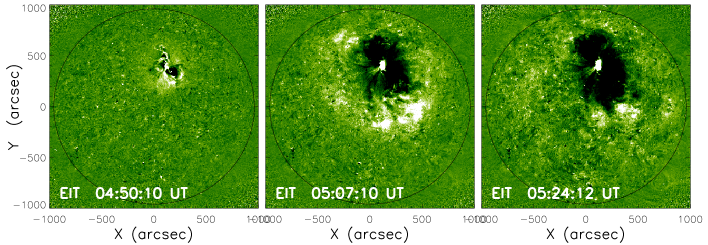
Figure 1: EIT 195 Å base difference images showing the evolution of the most famous EIT wave event on 1997 May 12 (from Chen, 2011).

After the launch of the Solar and Heliospheric Observatory (SOHO) spacecraft, one of its payload, EUV Imaging Telescopes (EIT; Delaboudinière et al., 1995), began to monitor the full solar disk in 4 EUV channels, with a cadence of $\sim$15 min for the 195Å channel. Using the running difference technique, Thompson et al. (1998) found that a large-scale wave, with bright fronts immediately followed by extending dimmings, propagates out from the flaring site, with a velocity of 250 km s^-1, as illustrated by Fig. 1. They were named “EIT waves” after the telescope. Such an interesting phenomenon sparked wide interest, as well as controversies, in the community. It is hotly debated whether EIT waves are the long-awaited coronal counterparts of H$\alpha$ Moreton waves or not. In this section, we summarize the typical observational features of “EIT waves”. It is expected that any successful model should explain all these characteristics.

(1) The velocity

Klassen et al. (2000) carried out a statistical study on the EIT wave velocity based on the EIT observations in 1997, and it was found that the velocity varies from 138 to 465 km s^-1, with an average of 271 km s^-1. With a higher cadence of 2.5 min, the Extreme Ultraviolet Imager (EUVI) on board the STEREO spacecraft revealed that the EIT wave velocity can be as small as $\sim 10$ km s^-1 (Zhukov et al., 2009), which is even much smaller than the sound speed in the corona. Long et al. (2008) pointed out that the low cadence observations by SOHO/EIT would underestimate the EIT wave velocity. However, we note that a fair argument is that low-cadence observations would underestimate the peak velocity and overestimate the trough velocity when the EIT wave speed changes with time.

Furthermore, Klassen et al. (2000) found that the EIT wave velocity is generally $>3$ times slower than the associated type II radio bursts, and the velocities of these two phenomena have no any correlation. Note that type II radio bursts have been well established to be due to the fast-mode shock wave in the corona.

It is also noticed that several authors have shown that EIT waves accelerate when they move from the proximity of source active region to the quiet region, and then decelerate (Long et al., 2008; Zhukov et al., 2009; Yang & Chen, 2010; Liu et al., 2010).

(2) Stationary fronts

EIT waves were found to finally stop somewhere, e.g., Thompson et al. (1999) found that EIT waves stop at the boundary of coronal holes, and Delannée & Aulanier (1999) revealed that a propagating EIT wave stopped at the footpoints of coronal magnetic separatrix. These two features are consistent since the boundary of coronal holes is also a magnetic separatrix.

Gopalswamy et al. (2009) analyzed STEREO/EUVI running difference images and claimed that an EIT wave was bounced back as it hit the boundary of a low-altitude coronal hole. On the contrary, Attrill (2010) studied that same event with the base difference images and argued that the reflecting EIT waves in Gopalswamy et al. (2009) might be an illusion, and the EIT wave actually stopped near the coronal hole boundary.

(3) Relation with solar flares

Cliver et al. (2005) pointed out that half of the EIT waves are associated with weak flares, such as GOES A- or B-class events, posing doubt on whether the pressure pulse in flares can generate the global-scale EIT waves. Following this line of thought, Chen (2006) did a test to examine whether solar flares alone can generate EIT waves. The results indicate that, without CMEs, even M- and X-class flares cannot produce EIT waves. Note that occasionally people claim that a flare without a CME was associated with an EIT wave. It is presumably that the CME was missed by the coronagraph due to low Thomson-scattering (Zhang et al., 2010).

(4) Relation with CMEs

Based on the statistical investigations, Biesecker et al. (2002) concluded that EIT waves are intimately related to CMEs, rather than flares. The test by Chen (2006) also indicates that no matter the associated flare is strong or weak, EIT waves can be observed only if a CME is present.

Nowadays, it is widely accepted that EIT waves are directly linked to CMEs. However, there still exists a dispute on the spatial relation between EIT waves and CMEs. Chen (2009a) and Dai et al. (2010) found that the EIT wave front is cospatial with the CME frontal loop, whereas Patsourakos & Vourlidas (2009) and Veronig et al. (2010) argued that the EIT wave front is further away from the CME frontal loop. This issue should be clarified.

(5) Other features

(a) Attrill et al. (2007) found that as the EIT wave front propagates outward, the location of the peak intensity rotates apparently in the same direction (clockwise or anti-clockwise) as the erupting filament;

(b) Harra & Sterling (2003) found that the Doppler velocity is negligible in the EIT wave fronts and significant in the extending dimmings that are immediately behind the EIT wave fronts;

(c) Yang & Chen (2010) examined the relation between the EIT wave velocity and the local magnetic field strength. They found that the two quantities often show a negative correlation, which does not favor the fast-mode wave model for EIT waves;

(d) There exists significant line broadening behind the EIT wave front (Chen et al., 2010).

3 Modelings of EIT waves

In order to interpret the intriguing phenomenon, several models have been proposed so far (see Wills-Davey & Attrill, 2009; Warmuth, 2010; Gallagher & Long, 2011; Chen, 2011, for reviews). Here, we briefly introduce several models. It is noted that EIT waves can be applied to diagnose the coronal magnetic field. However, the results critically depend on our understanding of EIT waves (Warmuth et al., 2004; Ballai, 2007; Chen, 2009b).

3.1 Fast-mode wave model

EIT waves were widely thought to be the coronal counterparts of H$\alpha$ Moreton waves, i.e., they are fast-mode waves in the corona (Wang, 2000; Wu et al., 2001; Warmuth et al., 2001; Vršnak et al., 2002; Warmuth et al., 2004; Ballai et al., 2005; Grechnev et al., 2008; Pomoell et al., 2008; Veronig et al., 2008; Gopalswamy et al., 2009; Patsourakos & Vourlidas, 2009; Muhr et al., 2010). In order to reconcile the large difference between Moreton waves and EIT waves, Wu et al. (2001) and Warmuth et al. (2001) proposed that the fast-mode wave speed decreases, say by $\sim$3 times, from the active region to the quiet region. Similarly, Grechnev et al. (2011) suggested that the EIT wave velocity profile fits the decelerating self-similar solutions very well. It is noted that the finding of a remote filament winking implies that the Moreton wave does not decelerate (Eto et al., 2002), the observations by STEREO/EUVI also do not show decelerations (Ma et al., 2009).

It is noted that the popular fast-mode wave model can hardly explain many features of EIT waves, such as their extremely low speed that is even smaller than the sound speed, their stationary fronts, their cospatiality with CME frontal loop, and so on.

3.2 Successive field-line stretching model

Figure 2: Schematics of the successive field-line stretching model for EIT waves (from Chen et al., 2005).

Inspired by the doubting of Delannée & Aulanier (1999) and Delannée (2000), Chen et al. (2002, 2005) proposed that EIT waves are apparent motions of brightenings that are generated by the compression as the magnetic field lines overlying the erupting flux rope are pushed to stretch up successively. This model was deduced naturally by realizing two facts: (1) All the field lines overlying the flux rope would be stretched outward successively during CMEs; (2) For each field line, the stretching starts from the top, and is then transferred down to the footpoints. The formation of EIT waves in this model is illustrated in Fig. 2, which can be understood as follows: As the flux rope (the circle in the figure) erupts, it pushes the first field line at point A, and then the perturbation propagates to point C with the local fast-mode wave speed. At the same time, the stretching propagates from point A to point B and then to point D with the local fast-mode wave speed. Wherever the stretching comes, the local plasma is compressed to form brightenings, i.e., EIT wave fronts. Therefore, the apparent speed for the EIT wave to propagate from point C to point D is $v_{\mathrm{EIT}}=CD/\Delta t$, with $\Delta t=\int_{A}^{B}1/v_{f}{\rm d}s+\int_{B}^{D}1/v_{A}{\rm d}s-\int_{A}^{C}1/v_{A}{\rm d}s$, where $v_{A}$ is the Alfvén speed, and $v_{f}$ is the fast-mode wave speed perpendicular to the field line, and the last two integrals are along the field line shown in Fig. 2. If the field lines are semicircular, it is derived that the EIT wave speed is about 1/3 of the local fast-mode wave speed. The erupting flux rope would also excite a piston-driven shock wave, which straddles over the flux rope and extends down to the solar surface. Different from the EIT waves, the fast-mode shock wave propagates outward with a speed slightly larger than the local fast-mode wave speed.

This model predicts that the CME-driven (not flare-driven) shock wave is the counterpart of H$\alpha$ Moreton wave, which runs ahead of the associated EIT waves, with a speed of $\sim$3 times faster. Harra & Sterling (2003) found evidence of a faster wave ahead of the EIT wave with the TRACE observations, and recently, Chen & Wu (2011) confirmed the the coexistence of a faster wave and an EIT wave with the Solar Dynamics Observatory (SDO, Title et al., 2006) observations. In 3-dimensional MHD simulations, Downs et al. (2011) also found that a fast-mode wave runs ahead of the EIT wave.

3.3 Successive reconnection model

Noticing that the EIT wave fronts rotate apparently in the same direction as the erupting filament, Attrill et al. (2007) also claimed that EIT waves should be related to the magnetic rearrangement, rather than an MHD wave. They proposed a successive reconnection model, i.e., EIT wave fronts are the footprint of the CME frontal loop, which is formed due to successive magnetic reconnection between the expanding core field lines and the small-scale opposite polarity loops. As more and more field lines are pushed to stretch up, some of them may have a chance to reconnect with neighboring loops (Cohen et al., 2009), it is a little hard to imagine that this accounts for most of EIT wave fronts.

3.4 Slow-mode (soliton) wave model

Noticing that EIT waves generally keep single-pulse fronts and that the EIT wave velocity is sometime smaller than the sound speed in the corona, Wills-Davey et al. (2007) speculated that the EIT waves might be best explained as a soliton-like phenomenon, say, a slow-mode solitary wave. They stated that a solitary wave model can also explain other properties of the EIT waves, such as their stable morphology, the non-linearity of their density perturbations, the lack of a single representative velocity, and their independence of Moreton waves. Such an idea requires further quantitative modelings, which are not so straightforward in 2- or 3-dimensions (Wills-Davey & Attrill, 2009).

Wang et al. (2009) performed 2-dimensional MHD numerical simulations of a flux rope eruption, where they found that behind the piston-driven shock appear velocity vortices and slow-mode shock waves. They interpret the vortices and the slow-mode shock wave as the EIT waves, which are 40% as fast as the Moreton waves.

3.5 Current shell model

Through 3-dimensional MHD simulations, Delannée et al. (2008) found that as a flux tube erupts, an electric current shell is formed by the return currents of the system, which separate the twisted flux tube from the surrounding fields. Slightly different from their early idea of magnetic rearrangement (Delannée & Aulanier, 1999), they claim that this current shell corresponds to the “EIT waves”. They also revealed that the current shell rotates, similar to the apparent rotation of the EIT wave fronts found by Podladchikova & Berghmans (2005). They emphasized the role of Joule heating in the current shell in explaining the EIT wave brightenings, which was not agreed by Wills-Davey & Attrill (2009).

4 Implications to the nature of CMEs

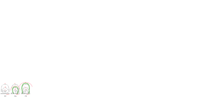
Figure 3: A schematic sketch of the formation mechanism of CME leading loops, where the CME leading loop (green) are apparently-moving density enhanced structure that is generated by the successive stretching of magnetic field lines as the erupting core structure, e.g., a flux rope, continues to push the overlying field lines to expand outward successively. The piston-driven shock is shown as pink lines (from Chen, 2009a).

The direct comparison between EIT waves and white-light CMEs revealed that EIT wave fronts are cospatial with the CME frontal loop (Chen, 2009a; Dai et al., 2010). Such a result confirmed the theoretical prediction of Chen & Fang (2005), i.e., EIT waves are the EUV counterparts of the CME frontal loops, whereas the EUV extending dimmings are the EUV counterparts of the CME cavity. The cospatiality implies that the formation mechanism of EIT waves can be directly applied to the CME frontal loops. Therefore, Chen (2009a) extended their field-line stretching model for EIT waves to explain the formation mechanism of the CME frontal loop. As illustrated by Fig. 3, as the core structure, e.g., a magnetic flux rope, erupts, the resulting perturbation propagates outward in every direction, with a probability of forming a piston-driven shock as indicated by the pink lines. However, different from a pressure pulse, the erupting flux rope keeps pushing the overlying magnetic field lines to expand, so that the field lines are stretched outward one by one. For each field line, the stretching starts from the top, e.g., point A for the first magnetic line, and then is transferred down to the leg (point D) with the Alfvén speed, by which the first field line is stretched entirely. The deformation at point A is also transferred upward to point B of the second magnetic field line with the fast-mode wave speed. Such a deformation would also be transferred down to its leg (point E) with the local Alfvén speed, by which the entire second magnetic field line is stretched up. The stretching of the magnetic field lines compresses the coronal plasma on the outer side of the field line, producing density enhancements. All the newly formed density enhancements at a given time form a pattern (green), which is observed as the CME frontal loop.

According to this model, the horizontal velocity of the CME footpoints is $\sim 1/3$ of the local fast-mode wave speed ($v_{f}$), and the radial velocity of the CME leading loop, i.e., the generally called CME velocity, is equal to the local fast-mode wave speed, which is several times faster than the plasma bulk velocity in the CME. Only when the local $v_{f}$ decreases below the bulk velocity, the CME becomes a real mass motion, which may happen at several solar radii. Besides, as noted by Chen (2011), this model might be applied to most CMEs. However, for some blowout CMEs with a very small velocity, their motion might be a mass motion from the very beginning.

5 Prospects

The controversies on “EIT waves” result mainly from the low cadence of the observations in the past decade. With the launch of SDO mission in 2010, the high-cadence (12 s) observations are unveiling the secret of “EIT waves” gradually (liu10; Chen & Wu, 2011). At the same time, spectroscopic observations will be of great help (Chen et al., 2010; Harra et al., 2011).

References

- Attrill (2010) Attrill G. D. R., 2010, ApJ, 718, 494
- Attrill et al. (2007) Attrill, G. D. R., Harra, L. K., van Driel-Gesztelyi, L., & Démoulin, P., 2007, ApJ, 656, L101
- Ballai et al. (2005) Ballai, I., Erdélyi, R., & Pintér, B. 2005, ApJ, 633, L145
- Ballai (2007) Ballai, I., 2007, Solar Phys., 246, 177
- Biesecker et al. (2002) Biesecker, D. A., Myers, D. C., Thompson, B. J. et al., 2002, ApJ, 569, 1009
- Chen et al. (2010) Chen, F., Ding, M. D., & Chen, P. F., 2010, ApJ, 720, 1254
- Chen (2006) Chen, P. F., 2006, ApJ, 641, L153
- Chen (2009a) Chen, P. F., 2009a, ApJ, 698, L112
- Chen (2009b) Chen, P., 2009b, Science in China G: Physics and Astronomy, 52, 1785
- Chen (2011) Chen, P. F., 2011, Living Reviews in Solar Physics, 8, 1
- Chen & Fang (2005) Chen, P. F., & Fang, C., 2005, IAU Symp., 226, 55
- Chen et al. (2005) Chen, P. F., Fang, C., & Shibata, K., 2005, ApJ, 622, 1202
- Chen et al. (2002) Chen, P. F., Wu, S. T., Shibata, K., & Fang, C., 2002, ApJ, 572, L99
- Chen & Wu (2011) Chen P. F., Wu Y., 2011, ApJ, 732, L20
- Ciaravella et al. (2006) Ciaravella, A., Raymond, J. C., & Kahler, S. W., 2006, ApJ, 652, 774
- Cliver et al. (2005) Cliver, E. W., Laurenza, M., Storini, M. & Thompson, B. J., 2005, ApJ, 631, 604
- Cohen et al. (2009) Cohen, O., Attrill, G. D. R., Manchester, W. B., IV, & Wills-Davey, M. J., 2009, ApJ, 705, 587
- Dai et al. (2010) Dai, Y., Auchère, F., Vial, J.-C. et al., 2010, ApJ, 708, 913
- Delaboudinière et al. (1995) Delaboudiniére, J.-P., et al., 1995, Solar Phys., 162, 291
- Delannée (2000) Delannée, C., 2000, ApJ, 545, 512
- Delannée & Aulanier (1999) Delannée, C., & Aulanier, G., 1999, Solar Phys., 190, 107
- Delannée et al. (2008) Delannée, C., Török, T., Aulanier, G., & Hochedez, J.-F., 2008, Solar Phys., 247, 123
- Downs et al. (2011) Downs, C., Roussev, I. I., van der Holst, B., et al., 2011, ApJ, 728, 2
- Eto et al. (2002) Eto, S., et al., 2002, PASJ, 54, 481
- Gallagher & Long (2011) Gallagher, P. T., & Long, D. M., 2011, Space Sci. Rev., in press
- Gopalswamy et al. (2009) Gopalswamy, N., et al., 2009, ApJ, 691, L123
- Grechnev et al. (2008) Grechnev, V. V., et al., 2008, Solar Phys., 253, 263
- Grechnev et al. (2011) Grechnev, V. V., et al., 2011, Solar Phys., in press
- Harra & Sterling (2003) Harra, L. K., & Sterling, A. C., 2003, ApJ, 587, 429
- Harra et al. (2011) Harra, L. K., Sterling, A. C., Gömöry, P., & Veronig, A. 2011, ApJ, 737, L4
- Hudson et al. (2003) Hudson, H. S., Khan, J. I., Lemen, J. R., Nitta, N. V., & Uchida, Y., 2003, Solar Phys., 212, 121
- Khan & Aurass (2002) Khan, J. I. & Aurass, H., 2002, Astron. Astrophys., 383, 1018
- Klassen et al. (2000) Klassen, A., Aurass, H., Mann, G., & Thompson, B. J., 2000, Astron. Astrophys., 141, 357
- Liu et al. (2010) Liu, W., Nitta, N. V., Schrijver, C. J., Title, A. M., & Tarbell, T. D., 2010, ApJ, 723, L53
- Long et al. (2008) Long, D. M., Gallagher, P. T., McAteer, R. T. J., & Bloomfield, D. S., 2008, ApJ, 680, L81
- Ma et al. (2009) Ma, S., Wills-Davey, M. J., Lin, J., et al., 2009, ApJ, 707, 503
- Moreton & Ramsey (1960) Moreton, G. E. & Ramsey, H. E., 1960, PASP, 72, 357
- Muhr et al. (2010) Muhr, N., Vršnak, B., Temmer, M., Veronig, A. M., & Magdalenić, J., 2010, ApJ, 708, 1639
- Narukage et al. (2004) Narukage N., Morimoto T., Kadota M., Kitai R., Kurokawa H., Shibata K., 2004, PASJ, 56, L5
- Neupert (1989) Neupert, W. M., 1989, ApJ, 344, 504
- Patsourakos & Vourlidas (2009) Patsourakos, S. & Vourlidas, A., 2009, ApJ, 700, 182
- Podladchikova & Berghmans (2005) Podladchikova, O., & Berghmans, D., 2005, Solar Phys., 228, 265
- Pomoell et al. (2008) Pomoell, J., Vainio, R., & Kissmann, R., 2008, Solar Phys., 253, 249
- Thompson et al. (1999) Thompson, B. J., Gurman, J. B., Neupert, W. M. et al., 1999, ApJ, 517, L151
- Thompson et al. (1998) Thompson, B. J., Plunkett, S. P., Gurman, J. B. et al., 1998, Geophys. Res. Lett., 25, 2465
- Title et al. (2006) Title, A. M., & The Aia Team, 2006, 36th COSPAR Scientific Assembly, 36, 2600
- Uchida (1968) Uchida, Y., 1968, Solar Phys., 4, 30
- Veronig et al. (2008) Veronig, A. M., Temmer, M., & Vršnak, B., 2008, ApJ, 681, L113
- Veronig et al. (2010) Veronig, A. M., Muhr, N., Kienreich, I. W., Temmer, M., & Vršnak, B., 2010, ApJ 716, L57
- Vršnak et al. (2002) Vršnak, B., Warmuth, A., Brajša, R., & Hanslmeier, A., 2002, Astron. Astrophys., 394, 299
- Wang (2000) Wang, Y. M., 2000, ApJ, 543, L89
- Wang et al. (2009) Wang, H., Shen, C., & Lin, J., 2009, ApJ, 700, 1716
- Warmuth (2010) Warmuth, A., 2010, Adv. Space Res., 45, 527
- Warmuth et al. (2001) Warmuth, A., Vršnak, B., Aurass, H., & Hanslmeier, A., 2001, ApJ, 560, L105
- Warmuth et al. (2004) Warmuth, A., Vršnak, B., Magdalenić, J. et al., 2004, Astron. Astrophys., 418, 1117
- Wills-Davey & Attrill (2009) Wills-Davey, M. J., & Attrill, G. D. R., 2009, Space Sci. Rev., 149, 325
- Wills-Davey et al. (2007) Wills-Davey, M. J., DeForest, C. E., & Stenflo, J. O., 2007, ApJ, 664, 556
- Wu et al. (2001) Wu, S. T., Zheng, H., Wang, S. et al., 2001, J. Geophys. Res., 106, 25089
- Yang & Chen (2010) Yang, H. Q., & Chen, P. F., 2010, Solar Phys., 266, 59
- Zhang et al. (2010) Zhang, Q.-M., Guo, Y., Chen, P.-F., et al., 2010, Res. Astron. Astrophys., 10, 461
- Zhukov et al. (2009) Zhukov, A. N., Rodriguez, L., & de Patoul, J., 2009, Solar Phys., 259, 73