Simplistic Coulomb forces in molecular dynamics: Comparing the Wolf and shifted-force approximations
Abstract
This paper compares the Wolf method to the shifted forces (SF) method for efficient computer simulation of isotropic systems interacting via Coulomb forces, taking results from the Ewald summation method as representing the true behavior. We find that for the Hansen-McDonald molten salt model the SF approximation overall reproduces the structural and dynamical properties as accurately as does the Wolf method. It is shown that the optimal Wolf damping parameter depends on the property in focus, and that neither the potential energy nor the radial distribution function are useful measures for the convergence of the Wolf method to the Ewald summation method. The SF approximation is also tested for the SPC/Fw model of liquid water at room temperature, showing good agreement with both the Wolf and the particle mesh Ewald methods; this confirms previous findings [Fennell & Gezelter, J. Chem. Phys. 124, 234104 (2006)]. Beside its conceptual simplicity the SF approximation implies a speed-up of a factor 2 to 3 compared to the Wolf method (which is in turn much faster than the Ewald method).
I Introduction
In molecular dynamics simulations the force evaluation consumes by far the most computational resources. For relatively short-ranged interactions like van der Waals interaction Mcquarrie (1976) it is common to introduce a cutoff radius such that if the distance between a particle pair exceeds , the particles do not interact Allen and Tildesley (1989). This truncation allows for different optimization methods like inclusion of cell and neighbor lists Allen and Tildesley (1989); Frenkel and Smit (1996); Rapaport (1995), which increase computational performance considerably. Traditionally, the pair potential is simply truncated and shifted such that it is zero at Allen and Tildesley (1989); Frenkel and Smit (1996); Rapaport (1995). This does not affect the force acting between particles at distances below , and if is sufficiently large, the fluid properties are virtually unaffected by this approximation. In fact, it has been shown Weeks et al. (1971); Mcquarrie (1976) that keeping merely the short-ranged, purely repulsive part of the van der Waals interaction can account for the fluid structure even near the critical point where correlations are long ranged. The truncated and shifted potential approximation ensures continuity of the potential energy, but introduces a discontinuity in the force at , leading to energy drift for long simulation times Toxvaerd and Dyre (2011). To overcome this one can instead apply a truncated and shifted force (SF) approximation Allen and Tildesley (1989), which has superior numerical stability Toxvaerd and Dyre (2011). Beside the numerical stability, it was recently shown by Toxvaerd and Dyre Toxvaerd and Dyre (2011) that for highly dense fluids the SF method allows for very small cut-off radius of (where is the atomic diameter) and corresponds approximately to the first local minimum in the radial distribution function. Applying such low cutoff to the truncated and shifted potential will lead to wrong physics and large energy drift toxvard_2011. The SF method therefore decreases the number of interactions significantly and thus the computational time. The potential corresponding to the SF interaction does however not match the original potential for from which the SF interaction was derived. Therefore, the thermodynamical properties cannot be compared directly, but can be derived from perturbation theory Nicolas et al. (1979); Allen and Tildesley (1989).
For long-ranged interactions, like the Coulomb interaction, one cannot simply introduce a standard cut and shifted potential. For example, simply truncating and shifting the Coulomb potential produces spurious fluid structure and wrong dynamics Feller et al. (1996). Numerous attempts have been made to overcome this problem. For example it has been suggested to use smoothing functions, but this leads in general to poor results, see Refs. Brooks et al., 1985; Zahn et al., 2002. Wolf et al. Wolf et al. (1999) cleverly showed that using a simple truncated and shifted Coulomb potential corresponds in practice to summing over interactions in a non-neutral sphere. To compensate for this these authors introduced a neutralizing term into the Coulomb potential; they further showed that faster convergence to the true energy is achieved by applying a damping factor . The Wolf method is computationally much faster than the classical Ewald summation technique and is today widely used within the scientific simulation community. The choice of the damping factor, , is, like the Ewald damping parameter Ewald (1921); Allen and Tildesley (1989), somewhat arbitrary, and the optimal value must be found by comparison with either experimental data or results from, e.g., the Ewald method Zahn et al. (2002); Demontis et al. (2001). If the Wolf damping parameter is zero, the Wolf method reduces to the SF approximation Fennell and Gezelter (2006), see also Denesyuk and Weeks Denesyuk and Weeks (2008) for a discussion. We note that an SF method for the Coulomb interactions was used as a clever trick in the biochemical simulation community Levitt et al. (1995); Beck et al. (2005) before the work by Wolf et al..
In this paper we apply the Wolf method in molecular dynamics simulations of a simple model of a molten salt and liquid water. In order to find the optimal value of the Wolf damping parameter we compare the simulated thermodynamical, dynamical, and structural properties with previously published results Hansen and McDonald (1975) based on the Ewald method. We show that the optimal value of depends on the property one wishes to calculate and the cutoff distance used. This sets the stage for documenting the main conclusion of this paper: for the systems studied here the SF approximation works as well as the Wolf method, confirming similar findings of Fennell and Gezelter Fennell and Gezelter (2006). Besides being conceptual simpler than the Wolf method, the SF method allows for more than a doubling of the computational speed.
II The Wolf approximation to the Coulomb potential
If is the distance between two particles, the force acting on one particle from the other is , where is for simplicity denoted the “force” and is minus the derivative of the corresponding potential function with respect to . For the Wolf method Wolf et al. (1999) the force is given by
| (1) | |||||
for and where is the complementary error function. Here and are the charges of the two particles in question, is the cutoff (i.e., for ), and is the Wolf damping parameter. In the paper by Wolf et al. it is implicitly understood that such that the cutoff only takes effect beyond range of damping. The damping parameter was introduced in order to ensure faster convergence to the limiting Madelung energy Wolf et al. (1999). Unfortunately, there is no theoretical prediction for the optimal value of , which must be found by comparison with other well-established methods like the Ewald summation method Wolf et al. (1999); Zahn et al. (2002); Demontis et al. (2001). Wolf et al. Wolf et al. (1999) and Demontis et al. Demontis et al. (2001) have shown via molecular dynamics simulations that the Wolf method reproduces the results obtained by the Ewald summation method for , where is the distance between oppositely charged particles in the first coordinate shell. Demontis et al. Demontis et al. (2001) also suggested that the optimal damping parameter is given by for sufficiently large systems.
From Eq. (1) it follows that for one has , and that for the force reduces to
| (2) |
This is the truncated and shifted force (SF) cutoff Allen and Tildesley (1989); Toxvaerd and Dyre (2011).
In Fig. 1(a) we plot the difference between the Wolf force, , and the corresponding Coulomb force, , for different damping parameters.
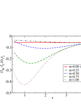
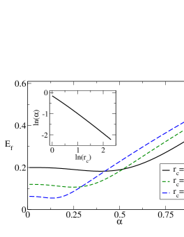
Clearly the damping parameter has a non-trivial effect on the force. For the difference is small compared to large values of , suggesting that the SF cutoff, Eq. (2), gives a good approximation to the Coulomb interaction. From Fig. 1(a) it is seen that an optimal value of exists that minimizes the difference. One way to identify this optimal value is by minimizing the function
| (3) |
which measures the total relative difference between and such that (since for all ). In Fig. 1(b) is plotted for three different cutoff distances. The optimal Wolf damping parameter converges to zero as increases, which reflects the simple fact that for and . More interestingly, the quantity does exhibit very little difference between the optimal value of and . The inset in Fig. 1(b) shows that the optimal Wolf parameter determined by the minimum of Eq. (3) is given roughly by . This simple analysis is consistent with the dependence suggested by Demontis et al. Demontis et al. (2001) based of molecular dynamics simulations (but they predict a smaller estimate of by a factor of 3/8).
The conclusion from Fig. 1 is that setting , i.e., adopting the SF approximation, gives results that are close to those obtained by carefully optimizing . This and the recent work by Toxvaerd and Dyre toxvaerd_2001 motivate the below reported molecular dynamics simulations, which compare the Wolf method to the SF cutoff for other quantities and realistic systems. As “truth” we take the well-established, but computationally expensive, Ewald summation method.
III Results for the Hansen and McDonald molten salt model
A series of molecular dynamics simulations was performed of a model molten salt proposed by Hansen and McDonald Hansen and McDonald (1975). Briefly, in this two-component model the ions are simple spherical particles that interact via a Coulomb potential and a van der Waals type potential given by the inverse power law , where , defines the energy scale and is the usual Lennard-Jones length scale parameter Mcquarrie (1976). We refer the reader to the reference for the full details. In the simulations we applied the Wolf method and varied the cutoff between 2.5 and 8.0 . The simulation box used was twice the size of the cutoff whenever ; for smaller cutoffs the box length was fixed to 8.36 . The number density for all systems were , thus, the number of ions varied from 216 to 1508. The results presented below were found to be independent of system size. The temperature is controlled using a Nosé-Hoover thermostat Nosé (1984); Hoover (1985) with . The results are compared to previously published data where the Ewald summation method was used Hansen and McDonald (1975), which represent the “true” Coulomb interaction.
First, in Fig. 2 (a) we compare the total potential energy obtained from the Wolf method for three different cutoff radii and varying damping parameters with the potential energy from the Ewald summation method. We note that is obtained directly from the Wolf potential functionWolf et al. (1999); Zahn et al. (2002) corresponding to the force given in Eq. (1).
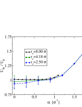
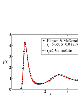
It is observed that is within the statistical uncertainty equal to for sufficiently small damping parameters, even for quite small cutoffs. This could lead to the conclusion that the Wolf method accounts correctly for electrostatic interactions for small cutoff distances. However, if one plots the radial distribution function , Fig. 2(b), we see that for the structure differs significantly from the result obtained using the Ewald summation method. This is true for all values of the damping parameter. From Fig. 2(b) we also notice that the SF approximation captures the structural properties correctly for , which is the smallest cutoff distance meeting the Wolf et al. Wolf et al. (1999) and Demontis et al. Demontis et al. (2001) criterion .
We study the radial distribution function dependence of and by defining the error parameter via
| (4) |
where is the radial distribution function for unlike charged particles of the Wolf method and the radial distribution function produced by the Ewald summation method. Similarly, the following error parameter quantifies the difference in diffusion constant
| (5) |
where and are the diffusion constants obtained from the Wolf and Ewald methods, respectively. Note that , whereas can be negative. The “correct” radial distribution function, , and diffusion constant, , were taken from Ref. Hansen and McDonald, 1975. Figure 3 shows the two error parameters for different cutoff radii and damping. The damping parameter was chosen because exhibits a minimum for this value for a large range of cutoffs. This is not the case for , however, which features a minimum for lower values of the damping parameter, depending on the cutoff (as expected from Fig. 1 (b)). This inconsistency is illustrated in the inset in which the error parameters are shown for as functions of . Obviously, any may be chosen to minimize , whereas features a minimum for . We note that and the cutoff radius fulfills the criterion defined by Wolf et al. and Demontis et al..
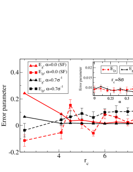
From Fig. 3 it is seen that is relatively large for small cutoffs (as expected), but that it for non-zero damping parameters quickly decreases and reaches almost zero for . For the SF approximation one needs in order to obtain the same accuracy in the radial distribution function. For large cutoffs the SF approximation results in better diffusion constants than the Wolf method with . We could, of course, have optimized with respect to the diffusion constant (giving for a large range of cutoffs). This, however, would decrease the agreement for the radial distribution function. This fact is highlighted in Table I, where the error parameters are listed for values of optimized, respectively, with respect to the diffusion constant and the radial distribution function (). For comparison we also give the error parameters for the SF approximation.
| ] | ||||
|---|---|---|---|---|
| 0.0 (SF) | 0.04 0.02 | 0.017 0.002 | ||
| 0.3 | 0.03 0.01 | 0.019 0.002 | ||
| 0.7 | 0.12 0.02 | 0.010 0.001 |
Within the statistical uncertainty there is no difference between the Wolf method using and the SF approximation.
Up to this point we have only discussed the structural and diffusive properties in the long time limit. To compare the short-time dynamics of the two methods we plot the velocity autocorrelation function and the intermediate scattering function in Fig. 4.
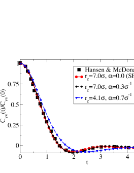
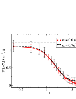
From Figs. 2 and 3 it was concluded that for small () and large () both the potential energy and the radial distribution function are in excellent agreement with the Ewald summation method, but in Fig. 4 we clearly observe the short-time dynamics is not correct for this set of parameter values. This shows that the cutoff must be sufficiently large for the Wolf method to correctly account for all the fluid properties – but at such large cutoff the SF approximation may be applied instead since it results in the same accuracy.
IV Results for a water model
We also tested the SF approximation for liquid water at the state point = (300 K, 998 kg m-3) using the flexible single point charge (SPC/Fw) water model Wu et al. (2006). In this model the chemical bond and the bending angle are allowed to vibrate around their zero-force values. The model is easy to implement and has been shown to predict many bulk properties better than for example the SPC, SPC/E and TIP3P models Wu et al. (2006); Raabe and Sadus (2007). In Fig. 5(a) we plot the oxygen-oxygen radial distribution function for the Wolf and SF methods. For comparison, data from Ref. Wu et al., 2006 are shown (filled squares), where the Coulomb interactions were evaluated using the particle-mesh Ewald (PME) method Darden et al. (1993).
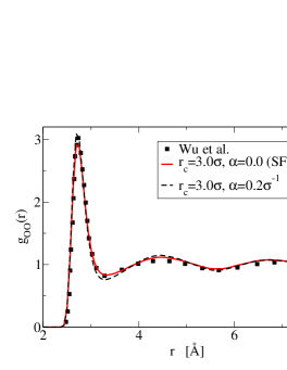
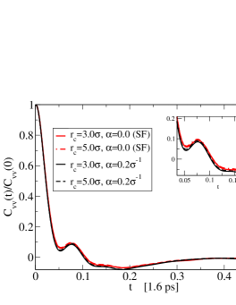
The radial distribution function is reproduced reasonably well by both methods. The SF approximation captures the liquid structure at least as well as the Wolf method, except at the first peak which is slightly underestimated. The radial distribution functions for both the SF and the Wolf methods are independent of the cutoff for radii larger than 9 Å, the value used by Zahn et al. Zahn et al. (2002); this corresponds to since the oxygen-hydrogen distance is around 1.8 Å. In Fig. 5(b) the center-of-mass velocity autocorrelation function is plotted for two different cutoffs for both methods. This dynamic property is largely independent of method and cutoff, as is the case for the liquid structure. The same conclusion was reached by Fennell and Gezelter Fennell and Gezelter (2006). For the SF approximation we obtain a diffusion constant of 2.4 m2 s-1 and a shear viscosity of 0.78 Pa s. This can be compared with the experimental values 2.3 m2 s-1 and 0.85 Pa s. It is also worth mentioning that Zahn et al. Zahn et al. (2002) used in their simulations of (rigid) SPC/E water, but found that the potential energy was in better agreement with the Ewald method for even lower damping parameters. For we observe no difference to the SF approximation.
V Concluding remarks
In conclusion, for simple molten salts and liquid water the SF approximation reproduces various properties as well as the Wolf method. The Wolf method has one more parameter than SF, and consequently this method may be optimized to give slightly better agreement with the Ewald summation method. Such an optimization, however, must be carried separately out for each property in focus and for each different system. Beside its simplicity (and thus easy-to-code feature), we found that the SF approximation leads to a simulation speed-up of 2-3 compared to the Wolf method. Of course, the actual speed-up depends on the specific problem and the use of optimization techniques, but the calculation of the four terms in Eq. (1) involves complicated mathematical functions and is deemed to consume considerably more computational resources than the simple SF approximation. We wish to stress here that the paper of Wolf et al. was the first to correctly analyze why the SF approximation for Coulomb forces is superior to the standard truncated and shifted potential interaction model.
Fennell and Gezelter Fennell and Gezelter (2006) carefully analyzed an impressive number of different systems including simple crystals showing a good agreement between the SF method and the Ewald technique. In their conclusion the authors suggested that the SF approximation can also be used for confined geometries, thereby overcoming the enforced periodicity in the unmodified Ewald method. We agree that the Ewald method can be problematic (even for periodic systems Karlström et al. (2008)), but, the SF approach (as well as the Wolf method) is an approximation that suppresses the intrinsic long-ranged nature of the Coulomb interactions leading to an artificially molecular orientation Feller et al. (1996); Takahashi et al. (2011) in confinements. For confined fluids alternative methods have recently been adviced, see Refs. Rodgers and Weeks, 2008; Wu and Brooks, 2005; Denesyuk and Weeks, 2008.
VI Acknowledgements
JSH wishes to acknowledge Lunbeckfonden for supporting this work as part of grant no. R49-A5634. The centre for viscous liquid dynamics “Glass and Time” is sponsored by the Danish National Research Foundation (DNRF).
References
- Mcquarrie (1976) D. A. Mcquarrie, Statistical Mechanics (Harper and Row, New York, 1976).
- Allen and Tildesley (1989) M. P. Allen and D. J. Tildesley, Computer Simulation of Liquids (Clarendon Press, New York, 1989).
- Frenkel and Smit (1996) D. Frenkel and B. Smit, Understanding Molecular Simulation (Academic Press, London, 1996).
- Rapaport (1995) D. Rapaport, The Art of Molecular Dynamics Simulation (Cambridge University Press, Cambridge, 1995).
- Weeks et al. (1971) J. D. Weeks, D. Chandler, and H. C. Andersen, J. Chem. Phys. 54, 5237 (1971).
- Toxvaerd and Dyre (2011) S. Toxvaerd and J. C. Dyre, J. Chem. Phys 134, 081102 (2011).
- Nicolas et al. (1979) J. J. Nicolas, K. E. Gubbins, W. B. Streett, and D. J. Tildesley, Mol. Phys. 37, 1429 (1979).
- Feller et al. (1996) S. E. Feller, R. W. Pastor, A. Rojnuckarin, S. Bogusz, and B. R. Brooks, J. Phys. Chem. 100, 17011 (1996).
- Brooks et al. (1985) C. L. Brooks, B. M. Pettitt, and M. Karplus, J. Chem. Phys. 83, 5897 (1985).
- Zahn et al. (2002) D. Zahn, B. Schilling, and S. M. Kast, J. Phys. Chem. B 106, 10725 (2002).
- Wolf et al. (1999) D. Wolf, P. Keblinski, S. R. Phillpot, and J. Eggebrecht, J. Chem. Phys. 110, 8254 (1999).
- Ewald (1921) P. Ewald, Ann. Phys. 369, 253 (1921).
- Demontis et al. (2001) P. Demontis, S. Spanu, and G. B. Suffritti, J. Chem. Phys. 114, 7980 (2001).
- Fennell and Gezelter (2006) C. J. Fennell and J. D. Gezelter, J. Chem. Phys. 124, 234104 (2006).
- Denesyuk and Weeks (2008) N. A. Denesyuk and J. D. Weeks, J. Chem. Phys 128, 124109 (2008).
- Levitt et al. (1995) M. Levitt, M. Hirshberg, R. Sharon, and V. Daggett, Comp. Phys. Comm. 91, 215 (1995).
- Beck et al. (2005) D. A. C. Beck, R. S. Armen, and V. Daggett, Biochem. 44, 609 (2005).
- Hansen and McDonald (1975) J. P. Hansen and I. R. McDonald, Phys. Rev. A 11, 2111 (1975).
- Nosé (1984) S. Nosé, Mol. Phys. 52, 255 (1984).
- Hoover (1985) W. G. Hoover, Phys. Rev. A 31, 1695 (1985).
- Wu et al. (2006) Y. Wu, H. L. Tepper, and G. A. Voth, J. Chem. Phys. 124, 024503 (2006).
- Raabe and Sadus (2007) G. Raabe and R. J. Sadus, J. Chem. Phys. 126, 044701 (2007).
- Darden et al. (1993) T. Darden, D. York, and L.Pedersen, J. Chem. Phys. 98, 10089 (1993).
- Karlström et al. (2008) G. Karlström, J. Stenhammer, and P. Linse, J. Phys.: Condens. Matter 20, 494204 (2008).
- Takahashi et al. (2011) K. Takahashi, T. Narumi, and K. Yasouko, J. Chem. Phys. 134, 174112 (2011).
- Rodgers and Weeks (2008) J. M. Rodgers and J. D. Weeks, PNAS 105, 19136 (2008).
- Wu and Brooks (2005) X. Wu and B. R. Brooks, J. Chem. Phys. 122, 044107 (2005).