Invariants, Projection Operators and

SU(N)$\times$SU(N) Irreducible Schwinger Bosons

Abstract

We exploit $SU(N)$ Schwinger bosons to construct and analyze the coupled irreducible representations of $SU(N)\times SU(N)$ in terms of the invariant group. The corresponding projection operators are constructed in terms of the invariant group generators. We also construct $SU(N)\times SU(N)$ irreducible Schwinger bosons which directly create these coupled irreducible states. The $SU(N)$ Clebsch Gordan coefficients are computed as the matrix elements of the projection operators.

PACS:  02.20.-a, 02.20.Sv, 03.65.-w, 31.10.+z

1 Introduction

It is well known that the Schwinger representation of the $SU(2)$ Lie algebra [1] has played important roles in widely different branches of physics such as nuclear physics [2], condensed matter physics [3], quantum optics [4], gauge theories [5], quantum gravity [6] etc. They have also played equally significant role in the study of Lie groups [7]. In particular, in the context of representation theory of $SU(N)$ group [8] the Schwinger bosons enable us to construct their unitary irreducible representations with enormous ease and simplicity [9, 10, 11, 12, 13, 14]. The $SU(2)$ case, studied extensively by Schwinger himself, provides the easiest example of this simplification. The Hilbert space ${\cal H}_{sb}$ associated with two Schwinger bosons is isomorphic to the representation space of $SU(2)$ and is the simplest possible representation or model space [15] of $SU(2)$. However, in the case of higher N $(N\geq 3)$, this simple isomorphism is lost due to the existence of certain $SU(N)$ invariant operators. These invariant operators follow $U(N-1)$ algebra [9, 11, 13, 14] and lead to $SU(N)$ invariant directions in the Hilbert space ${\cal H}_{sb}$ associated with $SU(N)$ group. Any two states which differ by an overall presence of such invariant operators will transform in the same way under $SU(N)$. This leads to the problem of multiplicity which in turn makes the representation theory of $SU(N)$ ($N\geq 3$) much more involved compared to $SU(2)$ [9, 10, 11, 13, 14]. The standard way to handle this problem is by demanding that the Schwinger boson states follow the symmetries of $SU(N)$ Young tableaues. In [13, 14] we showed that these $SU(N)$ Young tableaue symmetries can be easily realized by imposing certain $SU(N)$ invariant constraints on ${\cal H}_{sb}$. We further defined $SU(N)$ irreducible Schwinger bosons which weakly commute with the above constraints and hence directly create states which are invariant under all $SU(N)$ Young tableaue symmetries (see section 2.2). These $SU(N)$ irreducible states created by the monomials of $SU(N)$ irreducible Schwinger bosons are also multiplicity free. This makes the construction of all $SU(N)$ irreducible representations exactly analogous to the simple $SU(2)$ case. Thus the $SU(N)$ invariant constraint formulation provides a novel approach to study the $SU(N)$ representation theory. The purpose and motivation of the present work is to show that the above ideas can also be naturally extended to the study of the coupled representations of the the direct product group $SU(N)\times SU(N)$. We discuss the simplest and well studied $SU(2)\times SU(2)$ case first and then go to higher $SU(N)\times SU(N)$ groups. Infact, to our knowledge even the $N=2$ results (section 2) are new and have many novel features. In particular, we show that all coupled angular momentum irreducible representations can be projected out directly from the decoupled angular momentum states by certain projection operators. These projection operators are built from the invariant $Sp(2,R)\times SU(2)$ generators which commute with the total angular momentum generators. The $SU(2)$ Clebsch Gordan coefficients are simply the matrix elements of the above projection operators in the decoupled basis (see eqn. (15)) and can be easily computed (see section 2.3). Further, using the invariant algebra we also construct $SU(2)\times SU(2)$ irreducible Schwinger bosons which directly create all possible coupled $SU(2)\times SU(2)$ irreducible states. As expected, these simple $SU(2)$ techniques based on the invariant groups have natural extention to all higher $SU(N)$ groups. This is significant and important as, inspite of vast amount of literature on $SU(2)$ group and very specific techniques valid for $N=3,4$ etc., general computational methods to handle $SU(N)$ group for arbitrary N are hard to find [8, 16].

The plan of the paper is as follows. The section 2 deals with the simplest $SU(2)$ case. In this section we briefly construct the total angular momentum group invariant $Sp(2,R)\times SU(2)$ algebras [1]. Using this invariant algebra we construct projection operators which directly project the direct product Hilbert space to various irreducible Hilbert spaces characterized by the net angular momentum and net magnetic quantum numbers. Further, we construct $SU(2)\times SU(2)$ irreducible Schwinger bosons which trivially satisfy the above constraints and directly create the direct product irreducible representations. We then show that the Clebsch Gordan coefficients can be very easily computed as the matrix elements of the projection operators using the invariant algebra. In section 3 we show that the above $SU(2)$ techniques have very natural extention to all higher $SU(N)$ groups.

Direct product representations and invariant algebras

In the following sections we show that the symmetries of the direct product Young tableaues (see Figure 1 and Figure 2) can also be realized through certain group invariant constraints (see eqn. (16)). Further, these group invariant constraints lead to projection operators which project out the coupled irreducible representations from the direct product of two irreducible representations. As mentioned earlier, we discuss the simple $SU(2)$ group (section 2) first and then generalize these ideas and techniques to $SU(N)$ group with arbitrary N (section 3).

2 Representations of $SU(2)\times SU(2)$ and invariants

The Schwinger boson representations of $SU(2)\times SU(2)$ Lie algebra is:

$$J^{\mathrm{a}}_{1}~{}\equiv~{}\frac{1}{2}~{}a^{\dagger}_{\alpha}~{}(\sigma^{\mathrm{a}})_{\alpha\beta}~{}a_{\beta},~{}~{}~{}~{}~{}~{}J^{\mathrm{a}}_{2}~{}\equiv~{}\frac{1}{2}~{}b^{\dagger}_{\alpha}~{}(\sigma^{\mathrm{a}})_{\alpha\beta}~{}b_{\beta},$$ (1)

where $\sigma^{\mathrm{a}}$ denote the Pauli matrices, $(a_{\alpha},a^{\dagger}_{\alpha})$ and $(b_{\alpha},b^{\dagger}_{\alpha})$ with $\alpha=1,2$ are the two Schwinger boson doublets. It is easy to check that the operators in (1) satisfy the $SU(2)\times SU(2)$ Lie algebra with the SU(2) Casimirs:

$$\vec{J}_{1}\cdot\vec{J}_{1}\equiv{\hat{n}_{a}\over 2}\left({\hat{n}_{a}\over 2}+1\right),~{}~{}~{}~{}~{}~{}~{}~{}~{}\vec{J}_{2}\cdot\vec{J}_{2}\equiv{\hat{n}_{b}\over 2}\left({\hat{n}_{b}\over 2}+1\right).$$ (2)

In (2), $\hat{n}_{a}={\vec{a}^{\dagger}\cdot\vec{a}}=(a^{\dagger}_{1}a_{1}+a^{\dagger}_{2}a_{2})$ and $\hat{n}_{b}={\vec{b}^{\dagger}\cdot\vec{b}}=(b^{\dagger}_{1}b_{1}+b^{\dagger}_{2}b_{2})$ are the number operators with eigenvalues $n_{a}=n_{a}^{1}+n_{a}^{2}$ and $n_{b}=n_{b}^{1}+n_{b}^{2}$ respectively. The decoupled angular momentum states are:

$$|j_{1},m_{1}\rangle=\frac{\left(a^{\dagger}_{1}\right)^{j_{1}+m_{1}}\left(a^{\dagger}_{2}\right)^{j_{1}-m_{1}}}{\sqrt{(j_{1}+m_{1})!(j_{1}-m_{1})!}}|0\rangle,~{}~{}~{}~{}~{}~{}~{}~{}|j_{2},m_{2}\rangle=\frac{\left(b^{\dagger}_{1}\right)^{j_{2}+m_{2}}\left(b^{\dagger}_{2}\right)^{j_{2}-m_{2}}}{\sqrt{(j_{2}+m_{2})!(j_{2}-m_{2})!}}|0\rangle.$$ (3)

The representations of $SU(2)$ can also be characterized by the eigenvalues of the total occupation number operator as,

$$|n^{1}_{a},n^{2}_{a}\rangle=\frac{\left(a^{\dagger}_{1}\right)^{n_{a}^{1}}\left(a^{\dagger}_{2}\right)^{n_{a}^{2}}}{\sqrt{n_{a}^{1}!n_{a}^{2}!}}|0\rangle,~{}~{}~{}~{}~{}~{}|n_{b}^{1},n_{b}^{2}\rangle=\frac{\left(b^{\dagger}_{1}\right)^{n_{b}^{1}}\left(b^{\dagger}_{2}\right)^{n_{b}^{2}}}{\sqrt{n_{b}^{1}!n_{b}^{2}!}}|0\rangle.$$ (4)

In (4) $n_{a}^{1}=j_{1}+m_{1},n_{a}^{2}=j_{1}-m_{1},n_{b}^{1}=j_{2}+m_{2},n_{b}^{2}=j_{2}-m_{2}.$ The direct product states $|n^{1}_{a},n^{2}_{a}\rangle\otimes|n_{b}^{1},n_{b}^{2}\rangle$ will often be denoted by $\left|\begin{array}[]{cc}n^{1}_{a}&n^{2}_{a}\\ n^{1}_{b}&n^{2}_{b}\end{array}\right\rangle.$ The total angular momentum generators are:

$$J^{\mathrm{a}}_{T}=J^{\mathrm{a}}_{1}+J^{\mathrm{a}}_{2}.$$ (5)

The corresponding group will be denoted by $SU(2)_{T}$. We now construct all possible $SU(2)_{T}$ invariants out of the two Schwinger boson doublets in (1). The first set of invariant operators is:

$$k_{+}\equiv a^{\dagger}\cdot\tilde{b}^{\dagger},~{}~{}k_{-}\equiv a\cdot\tilde{b},~{}~{}k_{0}=\frac{1}{2}(\hat{n}_{a}+\hat{n}_{b}+2).$$ (6)

In (6) the invariants $k_{\pm}$ are the antisymmetric combination of the two doublets: $a^{\dagger}\cdot\tilde{b}^{\dagger}\equiv\epsilon_{\alpha\beta}a^{\dagger}_{\alpha}b^{\dagger}_{\beta}=(a^{\dagger}_{1}b^{\dagger}_{2}-a^{\dagger}_{2}b^{\dagger}_{1})$ and $a\cdot\tilde{b}\equiv\epsilon_{\alpha\beta}a_{\alpha}b_{\beta}=(a_{1}b_{2}-a_{2}b_{1}).$ It is easy to check that $k_{+},k_{-}$ and $k_{0}$ commute with $SU(2)_{T}$ generators $J^{\mathrm{a}}$ in (5) and satisfy Sp(2,R) algebra:

$$\left[k_{-},k_{+}\right]=2k_{0},~{}~{}~{}~{}~{}~{}\left[k_{0},k_{\pm}\right]=\pm k_{\pm}.$$ (7)

The discrete unitary irreducible representations $|k,q\rangle$ of Sp(2,R) relevant for us in this work are characterized by the eigenvalues of $k^{2}\equiv k_{1}^{2}+k_{2}^{2}-k_{0}^{2}=\frac{1}{2}(k_{+}k_{-}+k_{-}k_{+})-k_{0}^{2}$ and $q$ satisfying:

$$k_{0}~{}|k,q\rangle=q~{}|k,q\rangle,~{}~{}~{}~{}~{}~{}~{}~{}k^{2}~{}|k,q\rangle=k(1-k)~{}|k,q\rangle.$$ (8)

In (8), $q=k,k+1,k+2,\cdots$. The Sp(2,R) raising and lowering operators satisfy: $k_{\pm}|k,q\rangle=\left[(q\pm k)(q\mp k\pm 1)\right]^{\frac{1}{2}}|k,q\pm 1\rangle$ and $k_{-}|k,q=k\rangle=0$.

Similarly, another $SU(2)_{T}$ invariant algebra is obtained by defining [1]:

$${\kappa}_{+}\equiv a^{\dagger}\cdot{b},~{}~{}{\kappa}_{-}\equiv b^{\dagger}\cdot{a},~{}~{}\kappa_{0}\equiv\frac{1}{2}\left(\hat{n}_{a}-\hat{n}_{b}\right).$$ (9)

These generators satisfy the standard $SU(2)$ algebra:

$$\left[{\kappa}_{+},{\kappa}_{-}\right]=2\kappa_{0},~{}~{}~{}\left[\kappa_{0},\kappa_{\pm}\right]=\pm\kappa_{\pm}.$$ (10)

It is easy to check that the $Sp(2,R)$ and $SU(2)$ generators in (6) and (9) respectively commute with each other as well as with $SU(2)_{T}$ in (5). Therefore, the coupled irreducible representations of $SU(2)\times SU(2)$ can also be labeled by the quantum numbers of the $Sp(2,R)\times SU(2)$ group (see (LABEL:sp2rc) and (LABEL:su2c)).

2.1 The Projection operators, invariants and symmetries of Young tableaues

In this section we consider the coupled angular momentum states obtained by taking the direct product of two arbitrary angular momentum states $|j_{1},m_{1}\rangle$ and $|j_{2},m_{2}\rangle$ as shown in Figure 1.

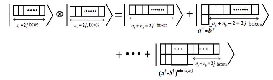
Figure 1: Graphical or Young tableaue representation of the identity (12). The $SU(2)\otimes SU(2)$ coupled states on the right hand side can be directly obtained from the decoupled state by the corresponding projection operators (see (14)). The coupled states on the right hand sides also carry $Sp(2,R)\times SU(2)$ quantum numbers (see (LABEL:sp2rc) and (LABEL:su2c)).

The Young tableaue decomposition in Figure 1 corresponds to the standard expansion of the decoupled basis in terms of the coupled basis:

$$|j_{1},m_{1}\rangle\otimes|j_{2},m_{2}\rangle=\sum_{j=j_{1}+j_{2}}^{|j_{1}-j_{2}|}C_{j_{1},m_{1};j_{2},m_{2}}^{~{}j,m}|j_{1},j_{2};j,m\rangle,$$ (11)

In (11) $m=m_{1}+m_{2}$. The same series can also be obtained by defining projection operators $\mathcal{P}^{j}$ which directly project the decoupled state to a particular coupled state $|j_{1},j_{2};j,m\rangle$. In terms of projection operators, the expansion (11) takes the form:

$$|j_{1},m_{1}\rangle\otimes|j_{2},m_{2}\rangle=\sum_{j=j_{1}+j_{2}}^{|j_{1}-j_{2}|}{\cal P}^{j}|j_{1},m_{1}\rangle\otimes|j_{2},m_{2}\rangle\equiv\sum_{r=0}^{min(2j_{1},2j_{2})}{\cal P}_{r}|j_{1},m_{1}\rangle\otimes|j_{2},m_{2}\rangle.$$ (12)

In (12) $r$ is the number of two boxes (invariants) on the right hand side of Figure 1, i.e.,

$$r=j_{1}+j_{2}-j.$$ (13)

Comparing the series (12) with the standard expansion in (11) we get:

$${\cal P}_{r}|j_{1},m_{1}\rangle\otimes|j_{2},m_{2}\rangle=C_{j_{1},m_{1};j_{2},m_{2}}^{~{}j,m}|j_{1},j_{2};j,m\rangle.$$ (14)

In (14) $j=j_{1}+j_{2}-r$ and $m=m_{1}+m_{2}$. Taking the norms of each side of (14) and using ${\cal P}_{r}^{2}={\cal P}_{r}$ we get:

$$C_{j_{1},m_{1};j_{2},m_{2}}^{~{}j,m}=\sqrt{\langle j_{1},j_{2},m_{1},m_{2}|{\cal P}_{r}|j_{1},j_{2},m_{1},m_{2}\rangle}.$$ (15)

In (15) we have used the notation $|j_{1},j_{2},m_{1},m_{2}\rangle\equiv|j_{1},m_{1}\rangle\otimes|j_{2},m_{2}\rangle$. The Clebsch Gordan coefficients in (15) will be explicitly computed in section 2.3.

We now construct the projection operators defined in (12). The Figure 1 and (12) imply that the projection operators can only depend on the $SU(2)_{T}$ invariant operators $\left(\hat{n}_{a},\hat{n}_{b},k_{\pm},{\kappa}_{\pm}\right)$ discussed in section 2. We first consider $r=0~{}(j=j_{1}+j_{2})$ case. The Figure 1 implies that ${\cal P}_{0}(\equiv{\cal P})$ should completely symmetrize the $SU(2)$ indices so that $j=j_{1}+j_{2}.$ Therefore, we demand:

$$k_{-}\left({\cal P}|j_{1},m_{1}\rangle\otimes|j_{2},m_{2}\rangle\right)=0.$$ (16)

As ${\cal P}$ depends only on the $SU(2)_{T}$ invariant operators, we can write the most general form as:

$${\cal P}=\sum_{q_{1},q_{2},q_{3},q_{4}}l_{\{q\}}(\hat{n}_{a},\hat{n}_{b})(k_{+})^{q_{1}}(k_{-})^{q_{2}}({\kappa}_{+})^{q_{3}}({\kappa}_{-})^{q_{4}}$$ (17)

In (17) $l_{\{q\}}\equiv l_{q_{1},q_{2},q_{3},q_{4}}(\hat{n}_{a},\hat{n}_{b})$ are the number operator dependent operators. Further, as the projection operator should not change the number of either a or b type oscillators, we get $q_{1}=q_{2},~{}q_{3}=q_{4}.$ On the other hand, the identity $\epsilon_{\alpha\beta}\epsilon_{\gamma\delta}=\delta_{\alpha\gamma}\delta_{\beta\delta}-\delta_{\alpha\delta}\delta_{\beta\gamma}$ implies:

$${\kappa}_{+}{\kappa}_{-}=\hat{n}_{a}\hat{n}_{b}-k_{+}k_{-}.$$ (18)

Thus all $SU(2)$ operators ${\kappa}_{+}{\kappa}_{-}$ in (17) can be removed in terms of Sp(2,R) operators $k_{+}k_{-}$. Therefore, the most general form of the projection operator is:

$${\cal P}=\sum_{q=0}^{\infty}l_{q}(\hat{n}_{a},\hat{n}_{b})~{}(k_{+})^{q}(k_{-})^{q}.$$ (19)

The constants $l_{q}$ can be computed (see appendix A.1) by using the constraint (16) and lead to:

$$l_{q}(\hat{n}_{a},\hat{n}_{b})=\frac{(-1)^{q}}{q!}\frac{(\hat{n}_{a}+\hat{n}_{b}-q)!}{(\hat{n}_{a}+\hat{n}_{b})!}$$ (20)

Note that the constant term in (20) is chosen to be unity (i.e $l_{0}=1$) so that:

$${\cal P}^{2}={\cal P}{\cal P}=\left(1+\sum_{q=1}^{\infty}l_{q}(\hat{n}_{a},\hat{n}_{b})~{}(k_{+})^{q}(k_{-})^{q}\right){\cal P}={\cal P}$$

as $k_{-}{\cal P}=0.$ The Figure 1 now immediately implies that all other projection operators are of the form:

$${\cal P}_{r}=N_{r}(k_{+})^{r}~{}{\cal P}~{}(k_{-})^{r}=N_{r}(k_{+})^{r}~{}{\cal P}~{}(k_{-})^{r}$$ (21)

The constant coefficients $N_{r}$ are fixed by demanding that the operators ${\cal P}_{r}$ satisfy ${\cal P}_{r}^{2}={\cal P}_{r}$ (see appendix A.1). We thus get:

$$N_{r}=\frac{(n_{a}+n_{b}-2r+1)!}{r!(n_{a}+n_{b}-r+1)!}$$ (22)

Note that these coefficient can also be computed by demanding completeness property:

$$\sum_{r=0}^{\textrm{min}(2j_{1},2j_{2})}{\cal P}_{r}={\it I}.$$ (23)

The completeness property (23) which is manifest in the defining expansion (12) is proved in appendix A.1. It is also easy to check that the Hilbert spaces projected by different projection operators in (21) are orthogonal:

$${\cal P}_{r}{\cal P}_{s}=\delta_{rs}{\cal P}_{r},~{}~{}~{}r,s=0,1,2,\cdots\textrm{ min}(2j_{1},2j_{2}).$$ (24)

In (24) we have used the Sp(2,R) commutation relation (6) and the constraints $k_{-}{\cal P}=0~{}(r>s),~{}~{}{\cal P}k_{+}=0(r<s).$ We note that the coupled angular momentum states ${\cal P}k_{-}^{r}|j_{1},m_{1}\rangle\otimes|j_{2},m_{2}\rangle$ in the expansion (12) also belong to the Sp(2,R) irreducible representations with lowest Sp(2,R) magnetic quantum number $q=q_{0}=(j_{1}+j_{2}-r+1)$ as:

$$k_{0}~{}{\cal P}~{}\left(k_{-}\right)^{r}|j_{1},m_{1}\rangle\otimes|j_{2},m_{2}\rangle = q_{0}~{}{\cal P}\left(k_{-}\right)^{r}|j_{1},m_{1}\rangle\otimes|j_{2},m_{2}\rangle.$$

$$k^{2}~{}{\cal P}\left(k_{-}\right)^{r}|j_{1},m_{1}\rangle\otimes|j_{2},m_{2}\rangle = q_{0}(1-q_{0})~{}{\cal P}\left(k_{-}\right)^{r}|j_{1},m_{1}\rangle\otimes|j_{2},m_{2}\rangle.$$

To get the second eigenvalue equation we have used $k_{-}{\cal P}=0$ to replace $k^{2}(\equiv\frac{1}{2}(k_{+}k_{-}+k_{-}k_{+})-k_{0}^{2})$ by $\frac{1}{2}[k_{-},k_{+}]-k_{0}^{2}=k_{0}(1-k_{0}).$ The equations (LABEL:abc1) immediately imply:

$$k_{0}~{}{\cal P}_{r}~{}|j_{1},m_{1}\rangle\otimes|j_{2},m_{2}\rangle = (j_{1}+j_{2}+1)~{}{\cal P}_{r}|j_{1},m_{1}\rangle\otimes|j_{2},m_{2}\rangle.$$

$$k^{2}~{}{\cal P}_{r}|j_{1},m_{1}\rangle\otimes|j_{2},m_{2}\rangle = q_{0}(1-q_{0})~{}{\cal P}_{r}|j_{1},m_{1}\rangle\otimes|j_{2},m_{2}\rangle.$$

Similarly, it is easy to check that the quantum numbers of $SU(2)_{T}$ invariant $SU(2)$ group in (9) are:

$$\kappa_{0}~{}{\cal P}_{r}~{}|j_{1},m_{1}\rangle\otimes|j_{2},m_{2}\rangle = (j_{1}-j_{2})~{}{\cal P}_{r}|j_{1},m_{1}\rangle\otimes|j_{2},m_{2}\rangle,$$

$$\kappa^{2}~{}{\cal P}_{r}|j_{1},m_{1}\rangle\otimes|j_{2},m_{2}\rangle = j(j+1)~{}{\cal P}_{r}|j_{1},m_{1}\rangle\otimes|j_{2},m_{2}\rangle.$$

Note that $j=j_{1}+j_{2}-r$ in (LABEL:su2c).

2.2 $SU(2)\times SU(2)$ irreducible Schwinger bosons

It is known that all possible $SU(N)$ irreducible representations can be written as monomials of $SU(N)$ irreducible Schwinger bosons [13, 14]. This construction is the $SU(N)$ extension of the Schwinger $SU(2)$ construction [1]. In this section we apply these ideas to construct the coupled states $|j_{1},j_{2},j,m\rangle$ in (14) as monomials of $SU(2)\times SU(2)$ irreducible Schwinger bosons (see equation (37)). The $SU(2)\times SU(2)$ irreducible Schwinger boson creation operators create states which satisfy $k_{-}=0$ and therefore correspond to maximally symmetric (or states with highest angular momentum) states. All other states can be constructed by applying the invariant operators on such maximally symmetric states. Note that this procedure is also illustrated by Figure 1. The first coupled state on the right hand side with $n_{a}+n_{b}=2j_{1}+2j_{2}$ is the maximally symmetric state. All other coupled states on the right hand side are obtained by multiplications of the invariant $k_{+}$ (i.e., two boxes arranged vertically in Figure 1) on such maximally symmetric states. As in [13, 14], we define:

$$A^{\dagger}_{\alpha}\equiv a^{\dagger}_{\alpha}+f(\hat{n}_{a},\hat{n}_{b})k_{+}\tilde{b}_{\alpha},~{}~{}B^{\dagger}_{\alpha}\equiv b^{\dagger}_{\alpha}+g(\hat{n}_{a},\hat{n}_{b})k_{+}\tilde{a}_{\alpha}.$$ (28)

Note that by construction (28) the $SU(2)\times SU(2)$ transformation properties of $A^{\dagger}_{\alpha}$ and $B^{\dagger}_{\alpha}$ are exactly same as those of $a^{\dagger}_{\alpha}$ and $b^{\dagger}_{\alpha}$ respectively. We now demand:

$$k_{-}~{}A^{\dagger}_{\alpha}~{}{\cal P}|j_{1},m_{1}\rangle\otimes|j_{2},m_{2}\rangle=0,~{}~{}~{}k_{-}~{}B^{\dagger}_{\alpha}~{}{\cal P}|j_{1},m_{1}\rangle\otimes|j_{2},m_{2}\rangle=0.$$ (29)

The above constraints can be solved in terms of the unknown operator valued functions $f(\hat{n}_{a},\hat{n}_{b})$ and $g(\hat{n}_{a},\hat{n}_{b})$:

$$f(\hat{n}_{a},\hat{n}_{b})=-\frac{1}{(\hat{n}_{a}+\hat{n}_{b})},~{}~{}~{}~{}~{}g(\hat{n}_{a},\hat{n}_{b})=\frac{1}{(\hat{n}_{a}+\hat{n}_{b})}.$$ (30)

Note that the $f(\hat{n}^{a},\hat{n}^{b})$ and $g(\hat{n}^{a},\hat{n}^{b})$ in (30) are well defined as they always follow a creation operator in (28). As an example of the states created by the $SU(2)\times SU(2)$ irreducible Schwinger bosons we consider the state: $A^{\dagger}_{\alpha}B^{\dagger}_{\beta}|0\rangle=A^{\dagger}_{\beta}B^{\dagger}_{\alpha}|0\rangle=\frac{1}{2}\left(a^{\dagger}_{\alpha}b^{\dagger}_{\beta}+a^{\dagger}_{\beta}b^{\dagger}_{\alpha}\right)|0\rangle$. We note that it is already symmetric in the $SU(2)$ indices $\alpha$ and $\beta$ and no explicit symmetrization is needed. Infact,

$$A^{\dagger}_{1}B^{\dagger}_{1}|0\rangle = ~{}~{}|j_{1}=1/2,j_{2}=1/2,j=1,m=1\rangle,$$

$$A^{\dagger}_{1}B^{\dagger}_{2}|0\rangle = \frac{1}{2}|j_{1}=1/2,j_{2}=1/2,j=1,m=0\rangle,$$ (31)

$$A^{\dagger}_{2}B^{\dagger}_{2}|0\rangle = ~{}~{}|j_{1}=1/2,j_{2}=1/2,j=1,m=-1\rangle.$$

The irreducible Schwinger bosons can also be directly constructed using the projection operators of the previous section as:

$$A^{\dagger}_{\alpha}\approx{\cal P}a^{\dagger}_{\alpha},~{}~{}~{}~{}B^{\dagger}_{\alpha}\approx{\cal P}b^{\dagger}_{\alpha}.$$ (32)

In (32) $\approx$ implies weak equality. In other words the equations (32) are true only on the projected section of the Hilbert space which satisfies the constraint $k_{-}=0$. The equivalence of (32) and (28) can be easily established by substituting ${\cal P}$ from (19) in (32) and noting that $l_{1}(\hat{n}_{a},\hat{n}_{b})=f(\hat{n}_{a},\hat{n}_{b})=-g(\hat{n}_{a},\hat{n}_{b})$. The completely symmetric states of $SU(2)_{T}$ can be easily defined through the irreducible Schwinger bosons:

$$|j_{1},j_{2},j=j_{1}+j_{2},m\rangle \equiv {N}^{j_{1}m_{1}}_{j_{2}m_{2}}~{}\frac{\left(A^{\dagger}_{1}\right)^{j_{1}+m_{1}}\left(A^{\dagger}_{2}\right)^{j_{1}-m_{1}}\left(B^{\dagger}_{1}\right)^{j_{2}+m_{2}}\left(B^{\dagger}_{2}\right)^{j_{2}-m_{2}}}{\sqrt{(j_{1}+m_{1})!(j_{1}-m_{1})!(j_{2}+m_{2})!(j_{2}-m_{2})!}}~{}|0\rangle.$$ (33)

To compute the normalization constant ${N}^{j_{1},m_{1}}_{j_{2},m_{2}}$ in (33) we note that the right hand side of the above equation can also be written in terms of decoupled states as:

$$\left(N_{j_{1}m_{1}}^{j_{2}m_{2}}\right)^{-1}|j_{1},j_{2};j=j_{1}+j_{2},m\rangle = {\cal P}~{}\frac{\left(A^{\dagger}_{1}\right)^{j_{1}+m_{1}}\left(A^{\dagger}_{2}\right)^{j_{1}-m_{1}}\left(B^{\dagger}_{1}\right)^{j_{2}+m_{2}}\left(B^{\dagger}_{2}\right)^{j_{2}-m_{2}}}{\sqrt{(j_{1}+m_{1})!(j_{1}-m_{1})!(j_{2}+m_{2})!(j_{2}-m_{2})!}}~{}|0\rangle$$ (34)

$$= {\cal P}~{}\frac{\left(a^{\dagger}_{1}\right)^{j_{1}+m_{1}}\left(a^{\dagger}_{2}\right)^{j_{1}-m_{1}}\left(b^{\dagger}_{1}\right)^{j_{2}+m_{2}}\left(b^{\dagger}_{2}\right)^{j_{2}-m_{2}}}{\sqrt{(j_{1}+m_{1})!(j_{1}-m_{1})!(j_{2}+m_{2})!(j_{2}-m_{2})!}}~{}|0\rangle$$

$$= {\cal P}|j_{1},m_{1}\rangle\otimes|j_{2},m_{2}\rangle.$$

In the first step above we have introduced identity as ${\cal P}$. We then replace the irreducible Schwinger bosons by their defining equations (28) and used ${\cal P}k_{+}=0$ in the second step to get the decoupled states at the end. To compute the normalization $N^{j_{1}m_{1}}_{j_{2}m_{2}}$ in (33) we notice that the completely symmetric states are given by (14) at $r=0$:

$${\cal P}~{}|j_{1},m_{1}\rangle\otimes|j_{2},m_{2}\rangle=C^{j=j_{1}+j_{2},m}_{j_{1},m_{1},j_{2},m_{2}}|j_{1},j_{2};j=j_{1}+j_{2},m\rangle.$$

Comparing this with (34) we get: ${N}^{j_{1},m_{1}}_{j_{2},m_{2}}~{}C^{j=j_{1}+j_{2},m}_{j_{1},m_{1},j_{2},m_{2}}=1$. Therefore,

$${N}^{j_{1}m_{1}}_{j_{2}m_{2}}=\frac{1}{C^{j=j_{1}+j_{2},m}_{j_{1},m_{1},j_{2},m_{2}}}=\left[\frac{(2j_{1}+2j_{2})!(j_{1}+m_{1})!(j_{1}-m_{1})!(j_{2}+m_{2})!(j_{2}-m_{2})!}{(2j_{1})!(2j_{2})!(j_{1}+j_{2}+m_{1}+m_{2})!(j_{1}+j_{2}-m_{1}-m_{2})!}\right]^{1/2}$$ (35)

For example, we put $j_{1}=2,m_{1}=0,j_{2}=1,m_{2}=0$ in (33) and replace the irreducible Schwinger bosons by their defining equations (28) and (30) to get:

$$|j_{1}=2,j_{2}=1,j=3,m=0\rangle={N}^{20}_{10}\left[\frac{3}{5}|2,0\rangle|1,0\rangle+\frac{\sqrt{3}}{5}|2,-1\rangle|1,1\rangle+\frac{\sqrt{3}}{5}|2,1\rangle|1,-1\rangle\right].$$ (36)

Therefore, explicit normalization of the above state gives: ${N}^{20}_{10}=\sqrt{\frac{5}{3}}$ which is also the value obtained by (35) with $C^{~{}~{}j=3,m=0}_{j_{1}=2,m_{1}=0;j_{2}=1,m_{2}=0}=\sqrt{\frac{3}{5}}$. With this value of normalization, the expansion (36) further gives:

$$C^{~{}~{}j=3,m=0}_{j_{1}=2,m_{1}=-1;j_{2}=1,m_{2}=1}=C^{~{}~{}j=3,m=0}_{j_{1}=2,m_{1}=1;j_{2}=1,m_{2}=-1}=\sqrt{\frac{1}{5}}.$$

The same values are also obtained from the Clebsch Gordan series (41) obtained using the invariants in the next section. The above example provides a self consistency check on the procedure. The discussions in the previous section imply that an arbitrary coupled state can be written as:

$$|j_{1},j_{2};j,m\rangle={\cal N}^{~{}j}_{j_{1},j_{2}}\left(k_{+}\right)^{j_{1}+j_{2}-j}|(j_{1}-j_{2}+j)/2,(j_{2}-j_{1}+j)/2;j,m\rangle.$$ (37)

Note that the state $|(j_{1}-j_{2}+j)/2,(j_{2}-j_{1}+j)/2;j,m\rangle$ is maximally symmetric and is of the form (33). The normalization constants ${\cal N}^{~{}j}_{j_{1},j_{2}}$ can be easily computed using the commutation relations (7) as $k_{-}|(j_{1}-j_{2}+j)/2,(j_{2}-j_{1}+j)/2;j,m\rangle=0$. They are given by:

$${\cal N}^{~{}j}_{j_{1},j_{2}}=\sqrt{\frac{(2j_{1}+2j_{2}+1)!}{(j_{1}+j_{2}-j)!(3j_{1}+3j_{2}-j+1)!}}.$$

We again emphasize that all possible $SU(2)\times SU(2)$ coupled states in (37) are monomials of the irreducible Schwinger bosons. All the symmetries of the coupled Young tableaues on the right hand side of Figure 1 are already present in (37) and there is no need for explicit symmetrization or anti-symmetrization by hand. Thus the the irreducible Schwinger bosons (37) can be thought of as the generalization of $SU(2)$ Schwinger bosons (3) which directly lead to coupled angular momentum states.

The $SU(2)\times SU(2)$ irreducible Schwinger bosons satisfy the following algebra:

$$\left[A^{\dagger}_{\alpha},A^{\dagger}_{\beta}\right]=0,~{}\left[B^{\dagger}_{\alpha},B^{\dagger}_{\beta}\right]=0,~{}\left[A^{\dagger}_{\alpha},B^{\dagger}_{\beta}\right]=0.~{}~{}~{}~{}~{}~{}~{}~{}~{}~{}~{}~{}~{}~{}~{}~{}~{}$$

$$\left[A_{\alpha},A^{\dagger}_{\beta}\right]=\delta_{\alpha\beta}-\frac{1}{\hat{n}_{a}+\hat{n}_{b}+1}b^{\dagger}_{\alpha}b_{\beta}+\frac{1}{(\hat{n}_{a}+\hat{n}_{b})(\hat{n}_{a}+\hat{n}_{b}+1)}k_{+}\tilde{b}_{\beta}a_{\alpha}$$ (38)

$$\left[B_{\alpha},B^{\dagger}_{\beta}\right]=\delta_{\alpha\beta}+\frac{1}{\hat{n}_{a}+\hat{n}_{b}+1}a^{\dagger}_{\alpha}a_{\beta}-\frac{1}{(\hat{n}_{a}+\hat{n}_{b})(\hat{n}_{a}+\hat{n}_{b}+1)}k_{+}\tilde{a}_{\beta}b_{\alpha}.$$

2.3 The projection operators and $SU(2)$ Clebsch Gordan Coefficients

The Clebsch Gordan coefficients are given by the defining equation (14):

$$C_{j_{1},m_{1};j_{2},m_{2}}^{j=j_{1}+j_{2}-r,m}=\langle j_{1},j_{2};j=j_{1}+j_{2}-r,m|{\cal P}_{r}|j_{1},m_{1},j_{2},m_{2}\rangle$$ (39)

This can be rewritten as:

$$C_{j_{1},m_{1};j_{2},m_{2}}^{j=j_{1}+j_{2}-r,m} = \frac{\langle j_{1},m^{\prime}_{1}=j_{1},j_{2},m^{\prime}_{2}=m-j_{1}|{\cal P}_{r}{\cal P}_{r}|j_{1},m_{1},j_{2},m_{2}\rangle}{C^{j=j_{1}+j_{2}-r,m}_{j_{1},m_{1}^{\prime}=j_{1};j_{2},m_{2}^{\prime}=m-j_{1}}}$$ (40)

$$= \frac{\langle j_{1},j_{1},j_{2},m-j_{1}|{\cal P}_{r}|j_{1},m_{1},j_{2},m_{2}\rangle}{\left[\langle j_{1},j_{1},j_{2},m-j_{1}|{\cal P}_{r}|j_{1},j_{1},j_{2},m-j_{1}\rangle\right]^{\frac{1}{2}}}$$

We have used ${\cal P}_{r}^{2}={\cal P}_{r}$ in (40). As shown in appendix B.1, the above matrix elements of ${\cal P}_{r}$ can be easily computed to give:

$$C_{j_{1},m_{1};j_{2},m_{2}}^{~{}~{}j,m} =\delta_{m,m_{1}+m_{2}}\sqrt{\frac{(j_{1}-j_{2}+j)!(j_{2}-m_{2})!(j_{2}+m_{2})!(j_{1}+m_{1})!(2j+1)(j-m)!}{(j_{1}+j_{2}+j+1)!(j_{2}-j_{1}+j)!(j_{1}+j_{2}-j)!(j_{1}-m_{1})!(j+m)!}}$$ (41)

$$\sum_{q=0}^{\mbox{min}\{j_{1}-j_{2}+j,j_{2}-j_{1}+j\}}\frac{(-1)^{q+j_{1}-m_{1}}(2j-q)!(j_{1}+j_{2}-j+q)!}{q!(j_{1}-j_{2}+j-q)!(j-m-q)!(j_{2}-j+m_{1}+q)!}$$

The series representing Clebsch Gordon coefficient in (41) matches with the expansion given in [17]. In section 3.2 this $SU(2)$ computation will be extended to $SU(N)$.

3 Invariants and representations of $SU(N)\times SU(N)$

We now generalize the previous $SU(2)$ ideas and techniques to direct product of two conjugate representations of $SU(N)$. For simplicity we choose these to be $N$ and $N^{*}$ representations of $SU(N)$. We write the corresponding generators as:

$$Q^{\mathrm{a}}_{1}~{}\equiv~{}\frac{1}{2}~{}{a^{\dagger}}^{\alpha}~{}(\Lambda^{\mathrm{a}})_{\alpha}^{~{}\beta}~{}a_{\beta},~{}~{}~{}~{}Q^{\mathrm{a}}_{2}~{}\equiv-~{}\frac{1}{2}~{}b^{\dagger}_{\alpha}~{}(\tilde{\Lambda}^{\mathrm{a}})^{\alpha}_{~{}\beta}~{}b^{\beta}.$$ (42)

In (42) ${\mathrm{a}}=1,2,\cdots(N^{2}-1)$ and $\alpha,\beta=1,2\cdots N$. $\Lambda^{\mathrm{a}}$’s are the generalized Gell-Mann matrices for $N$-plets of $SU(N)$ and $-\tilde{\Lambda}^{\mathrm{a}}$ are the dual matrices corresponding to the $N^{\ast}$-plets of $SU(N)$. From (42) it is clear that $a^{\dagger}$’s transform as $N$ under one $SU(N)$ and $b^{\dagger}$’s transform as $N^{\ast}$ under another $SU(N)$. Like in $SU(2)$ case (4) the decoupled $N$ and $N^{*}$ irreducible representations are:

$$|\{n_{a}\}\rangle\equiv|n_{a}^{1},n_{a}^{2},\cdots n_{a}^{N}\rangle = \frac{\left(a^{\dagger 1}\right)^{n_{a}^{1}}\left(a^{\dagger 2}\right)^{n_{a}^{2}}\cdots\left(a^{\dagger N}\right)^{n_{a}^{N}}}{\sqrt{n_{a}^{1}!n_{a}^{2}!\cdots n_{a}^{N}!}}|0\rangle,$$

$$|\{n_{b}\}\rangle\equiv|n_{b}^{1},n_{b}^{2},\cdots n_{b}^{N}\rangle = \frac{\left(b^{\dagger}_{1}\right)^{n_{b}^{1}}\left(b^{\dagger}_{2}\right)^{n_{b}^{2}}\cdots\left(b^{\dagger}_{N}\right)^{n_{b}^{N}}}{\sqrt{n_{b}^{1}!n_{b}^{2}!\cdots n_{b}^{N}!}}|0\rangle$$ (43)

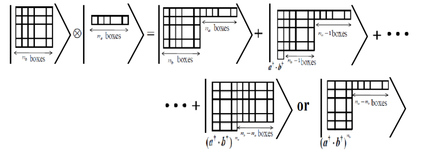
Figure 2: Graphical or Young tableau representation of the identity (49). The coupled $SU(N)\times SU(N)$ states on the right hand side can be directly obtained by projection operators (see (50)) and also carry Sp(2,R) quantum numbers (see (3)).

In (43) $\{n\}$ represents N partitions of n. The two Casimirs are the two total number operators $\hat{n}_{a}$ and $\hat{n}_{b}$ with eigenvalues $n_{a}$ and $n_{b}$ respectively:

$$n_{a}^{1}+n_{a}^{2}+\cdots+n_{a}^{N}=n_{a},~{}~{}~{}~{}~{}n_{b}^{1}+n_{b}^{2}+\cdots+n_{b}^{N}=n_{b}.$$ (44)

We will often denote the $SU(N)$ direct product state $|\{n_{a}\}\rangle\otimes|\{n_{b}\}\rangle$ by $\left|\begin{array}[]{cccc}n_{a}^{1}&n_{a}^{2}&\cdots&n_{a}^{N}\\ n_{b}^{1}&n_{b}^{2}&\cdots&n_{b}^{N}\end{array}\right\rangle.$ As in the case of $SU(2)$ (5), we define the total $SU(N)$ flux operators:

$$Q^{a}_{T}=Q^{a}_{1}+Q^{a}_{2}.$$ (45)

The corresponding group will be denoted by $SU(N)_{T}$. At this stage we can also define the coupled $SU(N)\times SU(N)$ states through the Clebsch Gordan decomposition (see Figure 2) as:

$$|\{n_{a}\}\rangle\otimes|\{n_{b}\}\rangle=\sum_{r=0}^{min(n_{a},n_{b})}{C}^{~{}~{}r}_{\{n_{a}\},\{n_{b}\}}~{}|\{n_{a}-r\}\{n_{b}-r\};r\rangle$$ (46)

As in Figure 2, the coupled states denoted by $|\{n_{a}-r\}\{n_{b}-r\};r\rangle$ in (46) represents the invariant operator $(k_{+})^{r}$ acting on the completely traceless tensor state of rank $(n_{a}-r,n_{b}-r)$.

We now define the following $SU(N)\times SU(N)$ invariant operators:

$$k_{+}\equiv a^{\dagger}\cdot{b}^{\dagger},~{}~{}k_{-}\equiv a\cdot{b},~{}~{}k_{0}=\frac{1}{2}(\hat{n}_{a}+\hat{n}_{b}+N).$$ (47)

In(47) the invariants are the scalar products of $N$ and $N^{*}$ representations: $a^{\dagger}\cdot{b}^{\dagger}=(a^{\dagger 1}b^{\dagger}_{1}+a^{\dagger 2}b^{\dagger}_{2}+\cdots+a^{\dagger N}b^{\dagger}_{N})$ and $a\cdot{b}=(a_{1}b^{1}+a_{2}b^{2}+\cdots+a_{N}b^{N}).$ It is easy to check that they again satisfy Sp(2,R) algebra (7):

$$\left[k_{-},k_{+}\right]=2k_{0},~{}~{}~{}~{}~{}~{}\left[k_{0},k_{\pm}\right]=\pm k_{\pm}.$$ (48)

Like in $SU(2)$ case, the $SU(N)\times SU(N)$ projection operators are defined as:

$$|\{n_{a}\}\rangle\otimes|\{n_{b}\}\rangle=\sum_{r=0}^{min(n_{a},n_{b})}{\cal P}_{r}~{}|\{n_{a}\}\rangle\otimes|\{n_{b}\}\rangle.$$ (49)

Comparing (46) with (49) we get:

$${\cal P}_{r}|\{n_{a}\}\rangle\otimes|\{n_{b}\}\rangle\equiv C^{~{}~{}~{}r}_{\{n_{a}\},\{n_{b}\}}|\{n_{a}-r\},\{n_{b}-r\};r\rangle.$$ (50)

In (50) $C^{~{}~{}~{}r}_{\{n_{a}\},\{n_{b}\}}$ are the Clebsch Gordan coefficients. Taking the norms on both the sides of (50) we get a simple expression for the $SU(N)$ Clebsch Gordan coefficients:

$$C^{~{}~{}~{}r}_{\{n_{a}\},\{n_{b}\}}=\sqrt{\langle\{n_{a}\}|\otimes\langle\{n_{b}\}|~{}{\cal P}_{r}~{}|\{n_{a}\}\rangle\otimes|\{n_{b}\}\rangle}$$ (51)

We will explicitly compute these coefficients in section 3.2.

We now construct the projection operators defined in (50). Note that the condition of tracelesness is exactly same as demanding the constraint $k_{-}=0$. Using this fact and the invariant algebra (48) the $SU(N)$ projection operator ${\cal P}_{0}$ can be easily constructed like in $SU(2)$ case (see appendix A.2):

$${\cal P}\equiv{\cal P}_{0}=\sum_{q=0}^{\infty}L_{q}\left(\hat{n}^{a},\hat{n}^{b}\right)(k_{+})^{q}(k_{-})^{q}$$ (52)

where

$$L_{q}\left(\hat{n}_{a},\hat{n}_{b}\right)=\frac{(-1)^{q}}{q!}\frac{(\hat{n}_{a}+\hat{n}_{b}+N-2-q)!}{(\hat{n}_{a}+\hat{n}_{b}+N-2)!}.)$$ (53)

Again, the projection operator in (52) satisfies

$${\cal P}^{2}={\cal P}{\cal P}=\left(1-\frac{1}{\hat{n}_{a}+\hat{n}_{b}+N-2}k_{+}k_{-}+\cdots\right){\cal P}={\cal P},$$

as $k_{-}{\cal P}=0$: Note that the $SU(N)$ projection operator (52) reduces to the $SU(2)$ projection operator (19) at $N=2$. Like in $SU(2)$ case, all other projection operators in (49) or equivalently in Figure 2 are of the form:

$${\cal P}_{r}=N_{r}~{}~{}(k_{+})^{r}~{}{\cal P}_{0}~{}(k_{-})^{r}=N_{r}~{}~{}(k_{+})^{r}~{}{\cal P}~{}(k_{-})^{r}$$ (54)

The constant coefficients $N_{r}$ are fixed by demanding that the operators ${\cal P}_{r}$ satisfy: ${\cal P}_{r}^{2}={\cal P}_{r}$ and are given by (see appendix A.2):

$$N_{r}=\frac{(n_{a}+n_{b}+N-2r-1)!}{r!(n_{a}+n_{b}+N-r-1)!}$$ (55)

As expected, (55) reduces to (22) at $N=2$. Like in $SU(2)$ case the projection operators satisfy the orthogonality and completeness properties:

$$\sum_{r=0}^{\mbox{min}(n_{a},n_{b})}{\cal P}_{r}={\it I},~{}~{}{\cal P}_{r}{\cal P}_{s}=\delta_{rs}{\cal P}_{r},~{}~{}~{}r,s=0,1,2,\cdots\mbox{min}(n_{a},n_{b}).$$ (56)

The orthogonality relation can be proven exactly like in the $SU(2)$ case (see (24)) and the completeness relation, manifest in (49), is proved in appendix A.2.

Note that the coupled states are also eigenstates of $k_{0}$ and $k^{2}$ and carry the following Sp(2,R) quantum numbers:

$$k_{0}~{}{\cal P}_{r}~{}|\{n_{a}\}\rangle\otimes|\{n_{b}\}\rangle = \frac{1}{2}\left(n_{a}+n_{b}+N\right)~{}{\cal P}_{r}|\{n_{a}\}\rangle\otimes|\{n_{b}\}\rangle.$$

$$k^{2}~{}{\cal P}_{r}|\{n_{a}\}\rangle\otimes|\{n_{b}\}\rangle = q_{0}(1-q_{0})~{}{\cal P}_{r}|\{n_{a}\}\rangle\otimes|\{n_{b}\}\rangle,$$

where, $q_{0}\equiv\frac{1}{2}\left(n_{a}+n_{b}+N-2r\right).$ It reduces to its $SU(2)$ value for $N=2,n_{a}=2j_{1},n_{b}=2j_{2}$.

3.1 $SU(N)\times SU(N)$ irreducible Schwinger bosons

Like in the section 2.2 (also see [13, 14]), we define:

$${A^{\dagger}}^{\alpha}\equiv{a^{\dagger}}^{\alpha}+F(\hat{n}_{a},\hat{n}_{b})k_{+}{b}^{\alpha},~{}~{}B^{\dagger}_{\alpha}\equiv b^{\dagger}_{\alpha}+G(\hat{n}_{a},\hat{n}_{b})k_{+}{a}_{\alpha}.$$ (58)

Note that by construction (58) the $SU(N)_{T}$ transformation properties of $A^{\dagger\alpha}$ and $B^{\dagger}_{\alpha}$ are exactly same as those of $a^{\dagger\alpha}$ and $b^{\dagger}_{\alpha}$ respectively. We now demand:

$$k_{-}~{}A^{\dagger\alpha}~{}{\cal P}|\{n^{i}_{a}\}\rangle\otimes|\{n^{i}_{b}\}\rangle=0,~{}~{}~{}k_{-}~{}B^{\dagger}_{\alpha}~{}{\cal P}|\{n^{i}_{a}\}\rangle\otimes|\{n^{i}_{b}\}\rangle=0.$$ (59)

The above constraints can be solved in terms of the unknown functions $F(\hat{n}_{a},\hat{n}_{b})$ and $G(\hat{n}_{a},\hat{n}_{b})$:

$$F(\hat{n}_{a},\hat{n}_{b})=G(\hat{n}_{a},\hat{n}_{b})=-\frac{1}{(\hat{n}_{a}+\hat{n}_{b}+N-2)}.$$ (60)

The first state of the Clebsch Gordon series for $SU(N)$$\times$$SU(N)$ as given in Figure 2 can be easily defined through the irreducible Schwinger bosons:

$$\Big{|}\{n_{a}\},\{n_{b}\};r=0\Big{\rangle} \equiv {N}^{\{n_{a}\}}_{\{n_{b}\}}\frac{\left(A^{\dagger 1}\right)^{n_{a}^{1}}\cdots\left(A^{\dagger N}\right)^{n_{a}^{N}}\left(B^{\dagger}_{1}\right)^{n_{b}^{1}}\cdots\left(B^{\dagger}_{N}\right)^{n_{b}^{N}}}{\sqrt{\left(n_{a}^{1}\right)!\left(n_{a}^{2}\right)!\cdots\left(n_{a}^{N}\right)!\left(n_{b}^{1}\right)!\left(n_{b}^{2}\right)!\cdots\left(n_{b}^{N}\right)!}}~{}\big{|}0\big{\rangle}$$ (61)

$$= {N}^{\{n_{a}\}}_{\{n_{b}\}}{\cal P}\frac{\left(a^{\dagger 1}\right)^{n_{a}^{1}}\cdots\left(a^{\dagger N}\right)^{n_{a}^{N}}\left(b^{\dagger}_{1}\right)^{n_{b}^{1}}\cdots\left(b^{\dagger}_{N}\right)^{n_{b}^{N}}}{\sqrt{\left(n_{a}^{1}\right)!\left(n_{a}^{2}\right)!\cdots\left(n_{a}^{N}\right)!\left(n_{b}^{1}\right)!\left(n_{b}^{2}\right)!\cdots\left(n_{b}^{N}\right)!}}\big{|}0\big{\rangle}$$

$$= {N}^{\{n_{a}\}}_{\{n_{b}\}}{\cal P}\Big{|}\{n^{i}_{a}\}\Big{\rangle}\otimes\Big{|}\{n^{i}_{b}\}\Big{\rangle}$$

The $r=0$ state in (61) is the first coupled representation on the right hand side of Figure 2. The ${\cal N}^{\{n_{a}\}}_{\{n_{b}\}}$ are the normalization constants. Again the construction (61) is the simplest and direct generalization of Schwinger boson construction (3) and (43) to $SU(N)\times SU(N)$ group. As an example we consider:

$$\left(N^{\{n_{a}=1\}}_{\{n_{b}=1\}}\right)^{-1}|\{n_{a}=1\},\{n_{b}=1\};r=0\rangle=A^{\dagger\alpha}B^{\dagger}_{\beta}|0\rangle=\left(a^{\dagger\alpha}b^{\dagger}_{\beta}-\frac{1}{N}\delta^{\alpha}_{\beta}k_{+}\right)|0\rangle.$$

Thus the tracelesness or equivalently the symmetries of Young tableaues are manifestly present in the definition of $SU(N)\times SU(N)$ irreducible Schwinger bosons.

Comparing (50) at $r=0$ with (61) we get:

$${N}^{\{n_{a}\}}_{\{n_{b}\}}~{}C^{~{}~{}~{}r=0}_{\{n_{a}\},\{n_{b}\}}=1.$$ (62)

Hence, like in $SU(2)$ case (35) the normalization factor ${N}^{\{n_{a}\}}_{\{n_{b}\}}$ is just the inverse of the CG coefficient at $r=0$. This normalization can be calculated using (74) from section 3.2. As an example we consider SU(3) states (43) with partitions: $n_{a}^{1}=1,n_{a}^{3}=0;n_{b}^{1}=1,n_{b}^{2}=1~{},~{}n_{b}^{3}=0$. In (61) we replace the irreducible Schwinger bosons by their defining equation (58) and (30) to get,

$$\Big{|}\{n_{a}^{1}=1,n_{a}^{2}=0,n_{a}^{3}=0\},\{n_{b}^{1}=1,n_{b}^{2}=1,n_{b}^{3}=0\};r=0\Big{\rangle}=N^{1,0,0}_{1,1,0}~{}~{}A_{1}^{\dagger}B^{\dagger 1}B^{\dagger 2}\big{|}0\big{\rangle}$$

$$=N^{1,0,0}_{1,1,0}~{}~{}\left[\frac{3}{4}\left|\begin{array}[]{ccc}1&0&0\\ 1&1&0\end{array}\right\rangle-\frac{\sqrt{2}}{4}\left|\begin{array}[]{ccc}0&1&0\\ 0&2&0\end{array}\right\rangle-\frac{1}{4}\left|\begin{array}[]{ccc}0&0&1\\ 0&1&1\end{array}\right\rangle\right].$$ (69)

Therefore, explicit normalization of the above state gives: $N^{1,0,0}_{1,1,0}=\sqrt{\frac{4}{3}}$. On the other hand, this normalization can also be computed by using (62) and the SU(3) Clebsch Gordan expression (74) obtained in the next section. Putting the above values of occupation numbers and $r=0$ in (74) we get:

$$\left(N^{1,0,0}_{1,1,0}\right)^{-1}=C^{r=0}_{\{n_{a}^{1}=1\},\{n_{b}^{1}=1,n_{b}^{2}=1\}}=\sqrt{\frac{2!}{4!3!3!}}(4!-3!)=\sqrt{\frac{3}{4}}.$$

Infact, at this stage we can cross check the other values of the $SU(N)$ Clebsch Gordan coefficients present in (69) with their values computed from the $SU(N)$ Clebsch Gordan expression (74) in the next section. The decomposition (69) implies

$$C^{~{}~{}r=0}_{\{010\}\{020\}}=-\sqrt{\frac{1}{6}}~{}~{}~{}{\mathrm{a}nd}~{}~{}~{}C^{~{}~{}r=0}_{\{001\}\{011\}}=-\sqrt{\frac{1}{12}}.$$

As can be checked, these are also the values obtained from (74) after putting $N=3$, various occupation numbers and $r=0$. Thus the above simple state provides three self consistency checks on our procedure.

The discussions in the previous section and Figure 2 imply that an arbitrary coupled state can be written as:

$$|\{n_{a}\},\{n_{b}\};r\rangle={\cal N}^{~{}r}_{n_{a},n_{b}}\left(k_{+}\right)^{r}|\{n_{a}-r\},\{n_{b}-r\};r=0\rangle$$ (70)

The normalization constants ${\cal N}^{~{}r}_{n_{a},n_{b}}$ can be easily computed as $k_{-}|\{(n_{a})\},\{(n_{b})\};r=0\rangle=0$ and are given by:

$${\cal N}^{~{}r}_{n_{a},n_{b}}=\sqrt{\frac{(n_{a}+n_{b}+N-1)!}{r!(n_{a}+n_{b}+N+r-1)!}}.$$

We again emphasize that except the invariant term all the $SU(N)\times SU(N)$ coupled states in (37) are monomials of the irreducible Schwinger bosons. The present construction of coupled states is a straightforward generalization of the original construction to the decoupled $SU(2)$ angular momentum states (3).

We note that the $SU(N)\times SU(N)$ irreducible Schwinger bosons satisfy:

$$\left[A^{\dagger}_{\alpha},A^{\dagger}_{\beta}\right]=0,~{}\left[B^{\dagger}_{\alpha},B^{\dagger}_{\beta}\right]=0,~{}\left[A^{\dagger\alpha},B^{\dagger}_{\beta}\right]=0\hskip 142.26378pt$$

$$\left[A_{\alpha},A^{\dagger\beta}\right]=\delta^{\beta}{}_{\alpha}-\frac{1}{\hat{n}_{a}+\hat{n}_{b}+N-1}b^{\dagger}_{\alpha}b^{\beta}+\frac{1}{(\hat{n}_{a}+\hat{n}_{b}+N-1)(\hat{n}_{a}+\hat{n}_{b}+N-2)}k_{+}a_{\alpha}b^{\beta}$$ (71)

$$\left[B^{\alpha},B^{\dagger}_{\beta}\right]=\delta^{\alpha}{}_{\beta}-\frac{1}{\hat{n}_{a}+\hat{n}_{b}+N-1}a^{\dagger\alpha}a_{\beta}+\frac{1}{(\hat{n}_{a}+\hat{n}_{b}+N-1)(\hat{n}_{a}+\hat{n}_{b}+N-2)}k_{+}a_{\beta}b^{\alpha}.$$

These relations reduce to (2.2) for $N=2$.

3.2 The Projection operators and $SU(N)$ Clebsch Gordon Coefficients

We write (49) and (50) as

$$\big{|}\{n_{a}\}\big{\rangle}\otimes\big{|}\{n_{b}\}\big{\rangle}=\sum_{r=0}^{n}\mathcal{P}_{r}\big{|}\{n_{a}\}\big{\rangle}\otimes\big{|}\{n_{b}\}\big{\rangle}\equiv\sum_{r=0}^{n}C^{~{}~{}~{}r}_{\{n_{a}\},\{n_{b}\}}\big{|}\{n_{a}-r\},\{n_{b}-r\};r\big{\rangle}$$ (72)

where, $n=\mbox{min}(n_{a},n_{b})$. Hence the Clebsch Gordon Coefficients can be computed as in the $SU(2)$ case:

$$C^{~{}~{}~{}r}_{\{n_{a}^{i}\},\{n_{b}^{i}\}}=\frac{~{}\big{\langle}n_{a},0,\cdots 0|\otimes\big{\langle}\bar{n}_{b}^{1},\bar{n}_{b}^{2},\cdots,\bar{n}_{b}^{N}\big{|}~{}\mathcal{P}_{r}~{}\big{|}n_{a}^{1},n_{a}^{2},\cdots n_{a}^{N}\big{\rangle}\otimes\big{|}n_{b}^{1},n_{b}^{2},\cdots n_{b}^{N}\big{\rangle}~{}~{}~{}}{\left[\big{\langle}n_{a},0,\cdots,0\big{|}\otimes\big{\langle}n_{b}^{1},\bar{n}_{b}^{2},\cdots,\bar{n}_{b}^{N}\big{|}~{}\mathcal{P}_{r}~{}\big{|}n_{a},0,\cdots,0\big{\rangle}\otimes\big{|}\bar{n}_{b}^{1},\bar{n}_{b}^{2},\cdots,\bar{n}_{b}^{N}\big{\rangle}\right]^{\frac{1}{2}}}$$ (73)

In the above equation $\{\bar{n}_{b}^{1},\cdots\bar{n}_{b}^{N}\}$ are the values of the occupation numbers corresponding to the special choice $\{n_{a}^{1}=n^{a},0,0,\cdots,0\}$ so that the total magnetic quantum numbers on both sides of the projection operator remain unchanged: They are given by:

$$\bar{n}_{b}^{1}=n_{a}-n_{a}^{1}+n_{b}^{1}~{}~{}~{}~{}~{}~{}{\mathrm{a}nd}~{}~{}~{}~{}~{}\bar{n}_{b}^{i}=n_{b}^{i}-n_{a}^{i}~{}~{}~{}~{}~{},i=2,3,...,N$$

As shown in appendix B.2, the matrix elements of $\mathcal{P}_{r}$ in (73) can be easily computed to give,

$$\hskip 28.45274ptC^{~{}~{}~{}r}_{\{n_{a}\},\{n_{b}\}} = \sqrt{\frac{(n_{a}+n_{b}+N-2r-1)n_{a}^{1}!n_{b}^{1}!n_{b}^{2}!...n_{b}^{N}!}{r!(n_{a}+n_{b}+N-r-1)!n_{a}^{2}!n_{a}^{3}!...n_{a}^{N}!\bar{n}_{b}^{2}!...\bar{n}_{b}^{N}!}}$$ (74)

$$\sqrt{\frac{(n_{a}-r)!(\bar{n}_{b}^{1}-r)!(n_{b}-\bar{n}_{b}^{1}+N-2)!}{(n_{b}+N-r-2)!(n_{a}+n_{b}-\bar{n}_{b}^{1}+N-r-2)!}}$$

$$\sum_{q}^{\mbox{min}(n_{a}-r,n_{b}-r)}\frac{(-1)^{q}}{q!}\frac{(q+r)!(n_{a}+n_{b}+N-2-2r-q)!}{(n_{a}-q-r)!(\bar{n}_{b}^{1}-q-r)!(n_{a}^{1}-n_{a}+q+r)!}$$

Note that this $SU(N)$ Clebsh Gordon series reduces to the $SU(2)$ Clebsch Gordon series (41) for $N=2$. This can be checked by identifying $(b^{\dagger}_{2},b^{\dagger}_{1})$ of $SU(N)$ with $(b^{\dagger}_{1},-b^{\dagger}_{2})$ of $SU(2)$ respectively so that $a^{\dagger}\cdot b^{\dagger}$ ($SU(N)$ invariant) $\rightarrow a^{\dagger}\cdot\tilde{b}^{\dagger}$ ($SU(2)$ invariant) and putting:

$$\begin{array}[]{ccc}n_{a}^{1}=j_{1}+m_{1}{}{}&n_{b}^{1}=j_{2}-m_{2}{}{}&\bar{n}_{b}^{1}=j_{2}-(m-j_{1})\\ \\ n_{a}^{2}=j_{1}-m_{1}{}{}&n_{b}^{2}=j_{2}+m_{2}{}{}&\bar{n}_{b}^{2}=j_{2}+(m-j_{1}).\end{array}$$ (77)

The $SU(2)$ Casimirs in (74) are: $n_{a}=n_{a}^{1}+n_{a}^{2}=2j_{1},~{}~{}n_{b}=n_{b}^{1}+n_{b}^{2}=\bar{n}_{b}^{1}+\bar{n}_{b}^{2}=2j_{2}$ and $r=j_{1}+j_{2}-j$.

4 Summary and discussions

In this work, we have investigated the role of $SU(N)\times SU(N)$ invariant groups in the Clebsch Gordan decomposition of direct product of two $SU(N)$ irreducible representations. The techniques were completely based on the invariant groups and their algebras enabling us to handle all $SU(N)$ within a single framework. It was crucial to use Schwinger construction to get all possible invariants. The invariant group generators were used to construct projection operators to get all possible coupled irreducible representations. The $SU(N)$ Clebsch Gordan coefficients were computed as matrix elements of these projection operators. Using the invariant algebra we also constructed $SU(N)\times SU(N)$ irreducible Schwinger bosons which directly creates the coupled irreducible states. Note that in the case of $SU(N)$ ($N\geq 3$) we only considered direct product of $N$ and $N^{*}$ representations leading to Sp(2,R) invariant algebras. In fact the analysis of section 3 is also valid for any two $SU(N)$ fundamental conjugate representations of dimensions ${}^{{}^{N}}C_{r}$ each. For simplicity we had chosen $r=1$. It will be interesting to extend these techniques to direct product of two arbitrary $SU(N)$ irreducible representations. The invariant group involved will then be much larger. All possible projection operators and the irreducible Schwinger bosons will again depend on the invariant operators or generators of the invariant group. The work in this direction is in progress and will be reported elsewhere.

Appendix A The projection operators

In this appendix we construct and prove the completeness property of $SU(N)\times SU(N)$ projection operators.

A.1 SU(2)$\times$SU(2)

We start with the construction of projection operator associated with symmetrization:

$$\mathcal{P}\left(|j_{1},m_{1}\rangle\otimes|j_{2},m_{2}\rangle\right)=C_{j_{1},m_{1};j_{2},m_{2}}^{~{}~{}j,m}|j_{1},j_{2},j=j_{1}+j_{2},m=m_{1}+m_{2}\rangle$$ (78)

We note that the $SU(2)\times SU(2)$ transformation property as well as the total number of $a^{\dagger}$’s ($=2j_{1}=n_{a}$) and $b^{\dagger}$’s ($=2j_{2}=n_{b}$) are same for the decoupled and coupled states on the left and right hand side of (78). Therefore the projection operator is of the form:

$$\mathcal{P}=\sum_{q=0}^{\mbox{min}\{n_{a},n_{b}\}}l_{q}(\hat{n}_{a},\hat{n}_{b})k_{+}^{q}k_{-}^{q}$$ (79)

where, $k_{\pm}$ are the $SU(2)$ invariant Sp(2,R) operators defined in (6). The unknown coefficients $l_{q}(\hat{n}_{a},\hat{n}_{b})$ can be easily fixed by demanding that the projected state is completely symmetric in all the $SU(2)$ indices and therefore should be annihilated by $k_{-}0$, i.e,

$$k_{-}~{}\mathcal{P}\mathcal{~{}}|j_{1},m_{1}\rangle\otimes|j_{2},m_{2}\rangle=0.$$ (80)

After using $k_{-}k_{+}^{q}=\left[k_{-},k_{+}^{q}\right]=q(\hat{n}_{a}+\hat{n}_{b}-q+3)k_{+}^{q-1}$ we get the recurrence relation:

$$l_{q+1}(\hat{n}_{a},\hat{n}_{b})=-\frac{1}{(q+1)(\hat{n}_{a}+\hat{n}_{b}-q)}l_{q}(\hat{n}_{a},\hat{n}_{b}),$$

leading to:

$$l_{q}(\hat{n}_{a},\hat{n}_{b})=\frac{(-1)^{q}}{q!}\frac{(\hat{n}_{a}+\hat{n}_{b}-q)!}{(\hat{n}_{a}+\hat{n}_{b})!}$$ (81)

Note that $l_{0}(\hat{n}_{a},\hat{n}_{b})=1$ implying the projection operator ${\cal P}^{2}={\cal P}$.

To compute the $\mathcal{P}_{r}$ normalization coefficients in (22) we use the required ${\cal P}^{2}_{r}={\cal P}_{r}$ property:

$${\cal P}_{r}~{}{\cal P}_{r} = N_{r}^{2}~{}\{(k_{+})^{r}~{}{\cal P}~{}(k_{-})^{r}\}~{}\{(k_{+})^{r}~{}{\cal P}~{}(k_{-})^{r}\}=N_{r}^{2}~{}(k_{+})^{r}~{}{\cal P}~{}\left[(k_{-})^{r},(k_{+})^{r}\right]~{}{\cal P}~{}(k_{-})^{r}$$ (82)

$$= \left(N_{r}r!\frac{(n_{a}+n_{b}-r+1)!}{(n_{a}+n_{b}-2r+1)!}\right)\underbrace{N_{r}~{}(k_{+})^{r}{\cal P}~{}(k_{-})^{r}}_{={\cal P}_{r}}={\mathcal{P}}_{r}.$$

In (82) we have used $k_{-}{\cal P}=0$ to replace $k_{-}^{r}k_{+}^{r}$ by the commutator $\left[k_{-}^{r},k_{+}^{r}\right]\left(=r!\frac{(\hat{n}_{a}+\hat{n}_{b}+r+1)!}{(n_{a}+n_{b}+1)!}\right)$ and replaced the number operators $\hat{n}_{a},\hat{n}_{b}$ by their eigenvalues $n_{a}=2j_{1},n_{b}=2j_{2}$ at the end. The above eqn. gives:

$$N_{r}=\frac{(n_{a}+n_{b}-2r+1)!}{r!(n_{a}+n_{b}-r+1)!}$$ (83)

One can easily check that ${\cal P}_{r}{\cal P}_{s\neq r}=0$ as $k_{-}{\cal P}=0(r>s)$ and ${\cal P}k_{+}=0(r<s)$ leading to orthonormal irreducible Hilbert spaces characterized by the net angular momentum quantum numbers.

We now prove the completeness property of the projection operators ${\cal P}_{r}$. We start with:

$$\sum_{r}\mathcal{P}_{r}|j_{1},m_{1}\rangle\otimes|j_{2},m_{2}\rangle = \sum_{r}~{}{\cal P}_{r}~{}\sum_{j=|j_{1}-j_{2}|}^{j_{1}+j_{2}}C_{j_{1},m_{1};j_{2},m_{2}}^{~{}~{}j,m}|j_{1},j_{2};j,m\rangle$$ (84)

$$= \sum_{r}{\cal P}_{r}~{}\sum_{j=|j_{1}-j_{2}|}^{j_{1}+j_{2}}C_{j_{1},m_{1};j_{2},m_{2}}^{~{}~{}j,m}{N}_{j,m}\left(J^{-}\right)^{j-m}|j_{1},j_{2};j,m=j\rangle$$

$$= \sum_{j=|j_{1}-j_{2}|}^{j_{1}+j_{2}}C_{j_{1},m_{1};j_{2},m_{2}}^{~{}~{}j,m}{N}_{j,m}\left(J^{-}\right)^{j-m}\underbrace{\sum_{r}{\cal P}_{r}~{}|j_{1},j_{2};j,m=j\rangle}_{={\cal P}_{0}|j_{1},j_{2};j,m=j\rangle=|j_{1},j_{2};j,m=j\rangle}$$

$$= |j_{1},m_{1}\rangle\otimes|j_{2},m_{2}\rangle.$$

In (84) the total lowering operator is defined as $J^{-}\equiv J_{a}^{-}+J_{b}^{-}(=a^{\dagger}_{1}a_{2}+b^{\dagger}_{1}b_{2})$ and $N_{j,m}(=\sqrt{\frac{(j+m)!}{(2j)!(j-m)!}}$ are the corresponding constants. We have also used the fact that the projection operators ${\cal P}_{r}$ commute with $J^{-}$ and satisfy orthonormality condition (24).

A.2 SU(N)$\times$SU(N)

We can exactly follow the $SU(2)$ techniques of the previous section and use the relation $\left[k_{-},k_{+}^{q}\right]=q(\hat{n}_{a}+\hat{n}_{b}+N+1-q)k_{+}^{q-1}$ to obtain the $SU(N)\times SU(N)$ projection operator (53):

$$L_{q}(n_{a},n_{b})=\frac{(-1)^{q}}{q!}\frac{(n_{a}+n_{b}+N-2-q)!}{(n_{a}+n_{b}+N-2)!}$$

. Similarly, as in $SU(2)$ case (24):

$${\cal P}_{r}~{}{\cal P}_{r} = N_{r}^{2}\{k_{+}^{r}{\cal P}k_{-}^{r}\}\{k_{+}^{r}{\cal P}k_{-}^{r}\}=N_{r}^{2}k_{+}^{r}{\cal P}~{}\left[k_{-}^{r},k_{+}^{r}\right]~{}{\cal P}~{}k_{-}^{r}$$ (85)

$$= N_{r}r!\frac{(n_{a}+n_{b}+N-r-1)!}{(n_{a}+n_{b}+N-2r-1)!}{\cal P}_{r}\equiv{\cal P}_{r}.$$

Above we have used the relation $\left[k_{-}^{r},k_{+}^{r}\right]=\frac{r!(\hat{n}_{a}+\hat{n}_{b}+N+r-1)!}{(\hat{n}_{a}+\hat{n}_{b}+N-1)!}.$ We thus get:

$$N_{r}=\frac{(n_{a}+n_{b}+N-2r-1)!}{r!(n_{a}+n_{b}+N-r-1)!}$$ (86)

As in $SU(2)$ case the different projected or irreducible spaces are orthonormal: ${\cal P}_{r}{\cal P}_{s\neq r}=0$ as $k_{-}{\cal P}=0(r>s)$ and ${\cal P}k_{+}=0(r<s).$ The completeness property of the $SU(N)$ projection operators also follows exactly as in the $SU(2)$ case.

Appendix B Matrix elements of Projection operators

In this appendix we compute the matrix elements of projection operators in (40) and (73) to get the $SU(2)$ and $SU(N)$ Clebsch Gordan coefficients.

B.1 SU(2)$\times$SU(2)

The numerator in (40) is:

$$\langle j_{1},j_{1},j_{2},m-j_{1}|{\cal P}_{r}|j_{1},m_{1},j_{2},m_{2}\rangle=N_{r}\left\langle\begin{array}[]{cc}2j_{1}&0\\ j_{2}+m-j_{1}&j_{1}+j_{2}-m\end{array}\right|k_{+}^{r}{\cal P}k_{-}^{r}\left|\begin{array}[]{cc}j_{1}+m_{1}&j_{1}-m_{1}\\ j_{2}+m_{2}&j_{2}-m_{2}\end{array}\right\rangle$$ (91)

$$= N_{r}\sum_{q}l_{q}(2j_{1}-r,2j_{2}-r)\underbrace{\left\langle\begin{array}[]{cc}2j_{1}&0\\ j_{2}+m-j_{1}&j_{1}+j_{2}-m\end{array}\right|k_{+}^{q+r}~{}k_{-}^{q+r}\left|\begin{array}[]{cc}j_{1}+m_{1}&j_{1}-m_{1}\\ j_{2}+m_{2}&j_{2}-m_{2}\end{array}\right\rangle}_{\equiv K(j_{1},m_{1},j_{2},m_{2},q,r)}$$ (96)

$$= N_{r}\sum_{q}~{}l_{q}(2j_{1}-r,2j_{2}-r)~{}K(j_{1},m_{1},j_{2},m_{2},q,r).$$ (97)

In the first step we have written the decoupled angular momentum states in terms of the occupation number basis. In the second step we have substituted the expansion (79) of ${\cal P}$ with $n_{a}=2j_{1}-r~{},~{}n_{b}=2j_{2}-r$ for the coefficient $l_{q}$ in (81). Note that the matrix elements K can be easily computed as both $k_{+}^{q+r}$ and $k_{-}^{q+r}$ in (97) can be replaced by monomials of harmonic oscillator creation and annihilation operators respectively:

$$k_{+}^{q+r}\rightarrow\left(a^{\dagger}_{1}~{}b^{\dagger}_{2}\right)^{q+r},~{}~{}~{}~{}~{}~{}~{}~{}~{}k_{-}^{q+r}\rightarrow(-1)^{q+r-s}~{}{}^{{}^{q+r}}C_{s}~{}\left(a_{1}b_{2}\right)^{s}\left(a_{2}b_{1}\right)^{q+r-s}.$$

Above $s=q+r+m_{1}-j_{1}$. Substituting these monomials in (97) leads to:

$$K = \frac{(-1)^{q+r-s}(q+r)!}{s!(q+r-s)!(j_{1}+m_{1}-s)!(j_{2}-m_{2}-s)!(j_{1}-m_{1}-q-r+s)!(j_{2}+m_{2}-q-r+s)!}$$ (98)

$$\times\sqrt{(2j_{1})!(j_{2}+m-j_{1})!(j_{2}-m+j_{1})!(j_{1}+m_{1})!(j_{1}-m_{1})!(j_{2}+m_{2})!(j_{2}-m_{2})!}.$$

Substituting $N_{r}$ from (83), $l_{q}(2j_{1}-r,2j_{2}-r)$ from (81) and K from above with $s=q+r+m_{1}-j_{1}$, the matrix element (97) takes the form:

$$\langle j_{1},j_{1},j_{2},m-j_{1}|{\cal P}_{r}|j_{1},m_{1},j_{2},m_{2}\rangle = \frac{(2j_{1}+2j_{2}-2r+1)!}{r!(2j_{1}+2j_{2}-r+1)!(2j_{1}+2j_{2}-2r)!}$$ (99)

$$\times\sqrt{\frac{(2j_{1})!(j_{2}-m+j_{1})!(j_{1}+m_{1})!(j_{2}+m_{2})!(j_{2}-m_{2})!}{(j_{2}+m-j_{1})!(j_{1}-m_{1})!}}$$

$$\sum_{q=0}^{\mbox{min}(2j_{1}-r,2j_{2}-r)}\frac{(-1)^{q+j_{1}-m_{1}}(q+r)!(2j_{1}+2j_{2}-2r-q)!}{(q+r+m_{1}-j_{1})!(j_{1}+j_{2}-m-q-r)!(2j_{1}-q-r)!}$$

Putting $r=j_{1}+j_{2}-j$ in the above equation we get:

$$\langle j_{1},j_{1},j_{2},m-j_{1}|{\cal P}_{j}|j_{1},m_{1},j_{2},m_{2}\rangle = \Bigg{[}\frac{(2j+1)!}{(2j)!(j_{1}+j_{2}-j)!(j_{1}+j_{2}+j+1)!}$$ (100)

$$\sqrt{\frac{(2j_{1})!(j_{1}+j_{2}-m)!(j_{1}+m_{1})!(j_{2}+m_{2})!(j_{2}-m_{2})!}{(j_{1}-m_{1})!(j_{2}-j_{1}+m)!}}~{}\Bigg{]}$$

$$\sum_{q=0}^{\mbox{min}(j_{1}-j_{2}+j,j_{2}-j_{1}+j)}\frac{(-1)^{q+j_{1}-m_{1}}}{(q)!}\frac{(j_{1}+j_{2}-j+q)!(2j-q)!}{(j_{2}-j+q+m_{1})!(j_{1}-j_{2}+j-q)!(j-m-q)!}$$

For the denominator of (40), we substitute $m_{1}=j_{1}$ and $m_{2}=m-j_{1}$ in (100) to obtain,

$$\hskip 82.51282pt\langle j_{1},j_{1},j_{2},m-j_{1}|\mathcal{P}_{r}|j_{1},j_{1},j_{2},m-j_{1}\rangle$$

$$=\frac{(2j+1)!(2j_{1})!(j_{2}+j_{1}-m)!}{(2j)!(j_{1}+j_{2}-j)!(j_{1}+j_{2}+j+1)!}~{}\sum_{q=0}^{q_{\textrm{m}ax}}~{}\frac{(-1)^{q}}{q!}\frac{(2j-q)!}{(j_{1}-j_{2}+j-q)!(j-m-q)!}.$$ (101)

In (101) the upper limit on the sum over q is $q_{{\max}}\equiv{min}(2j_{1}-r,2j_{2}-r)={min}(j_{1}-j_{2}+j,j_{2}-j_{1}+j).$ This above series in q is summed using the formula:

$$\sum_{q=0}\frac{(-1)^{q}}{q!}\frac{(C-q)!}{(A-q)!(B-q)!}=\frac{C!}{A!B!}\times\frac{(C-A)!(C-B)!}{C!(C-A-B)!}$$ (102)

Finally, the denominator in (40) is:

$$\hskip 85.35826pt\sqrt{\langle j_{1},j_{1},j_{2},m-j_{1}|\mathcal{P}_{r}|j_{1},j_{1},j_{2},m-j_{1}\rangle}$$

$$=\sqrt{\frac{(j+m)!(j_{2}-j_{1}+j)!(2j+1)!(2j_{1})!(j_{2}+j_{1}-m)!}{(2j)!(j_{1}+j_{2}-j)!(j_{1}+j_{2}+j+1)!(j-m)!(j_{2}-j_{1}+m)!(j_{1}-j_{2}+j)!}}$$ (103)

The final expression of the Clebsch Gordon coefficient in (41) is now obtained by dividing (100) by (B.1).

B.2 SU(N)$\times$SU(N)

Similarly the matrix element in the numerator of $SU(N)$ Clebsch Gordon coefficient expression (73) is:

$$\hskip 85.35826pt\Big{\langle}\{n_{a}^{1}=n_{a}\},\{\bar{n}_{b}\}\Big{|}\mathcal{P}_{r}\mathcal{P}_{r}\Big{|}\{n_{a}\},\{n_{b}\}\Big{\rangle}$$ (109)

$$= N_{r}\sum_{q}l_{q}(n_{a}-r,n_{b}-r)\underbrace{\left\langle\begin{array}[]{cccc}n_{a}&0&\ldots&0\\ \bar{n}_{b}^{1}&\bar{n}_{b}^{2}&\ldots&\bar{n}_{b}^{N}\end{array}\right|k_{+}^{q+r}k_{-}^{q+r}\left|\begin{array}[]{cccc}n_{a}^{1}&n_{a}^{2}&\ldots&n_{a}^{N}\\ n_{b}^{1}&n_{b}^{2}&\ldots&n_{b}^{N}\end{array}\right\rangle}_{K\left(\{n_{a}\},\{n_{b}\},q,r\right)}$$

$$\hskip 56.9055pt=N_{r}\sum_{q}l_{q}(n_{a}-r,n_{b}-r)K\left(\{n_{a}\},\{n_{b}\},q,r\right)$$

The matrix element $K\left(\{n_{a}\},\{n_{b}\},q,r\right)$ are calculated in the same way as in the $SU(2)$ case. In the computation of $K\left(\{n_{a}\},\{n_{b}\},q,r\right)$ in (109) $k_{+}^{q+r}$ and $k_{-}^{q+r}$ can be replaced by the following monomials of Schwinger bosons:

$$k_{+}^{q+r}\rightarrow(a^{\dagger}_{1}b^{\dagger 1})^{q+r},~{}~{}~{}~{}~{}~{}~{}~{}k_{-}^{q+r}\rightarrow\frac{(q+r)!}{\beta_{1}!\ldots\beta_{N}!}(a^{1}b_{1})^{\beta_{1}}(a^{2}b_{2})^{\beta_{2}}\ldots(a^{N}b_{N})^{\beta_{N}}$$ (110)

Equating the occupation numbers in the matrix element in (109) we get:

$$\beta_{1}=q+r+n_{a}^{1}-n_{a},~{}~{}\beta_{2}=n_{a}^{2},~{}~{}\beta_{3}=n_{a}^{3},~{}~{}~{}~{}\ldots,\beta_{N}=n_{a}^{N},$$

leading to:

$$K\left(\{n_{a}\},\{n_{b}\},q,r\right) = \sqrt{n_{a}!\bar{n}_{b}^{1}!\bar{n}_{b}^{2}!\ldots\bar{n}_{b}^{N}!n_{a}^{1}!n_{a}^{2}!\ldots n_{a}^{N}!n_{b}^{1}!n_{b}^{2}!\ldots n_{b}^{N}!}$$ (111)

$$\times\frac{(q+r)!}{(n_{a}^{1}-n_{a}+q+r)!n_{a}^{2}!\ldots n_{a}^{N}!}$$

$$\times\frac{1}{(n_{a}-q-r)!(\bar{n}_{b}^{1}-q-r)!\bar{n}_{b}^{2}!\ldots\bar{n}_{b}^{N}!}$$

Now substituting the values of $N_{r}$ and $l_{q}(n_{a}-r,n_{b}-r)$ from A.2 and the matrix element $K$ from above we finally get the numerator of (73) as:

$$\Big{\langle}\{n_{a}^{1}=n_{a}\},\{\bar{n}_{b}\}\Big{|}\mathcal{P}_{r}\Big{|}\{n_{a}\},\{n_{b}\}\Big{\rangle} = \frac{(n_{a}+n_{b}+N-2r-1)}{r!(n_{a}+n_{b}+N-r-1)!}\sqrt{\frac{n_{a}!\bar{n}_{b}^{1}!n_{a}^{1}!n_{b}^{1}!\ldots n_{b}^{N}!}{n_{a}^{2}!\ldots n_{a}^{N}!\bar{n}_{b}^{2}!\ldots\bar{n}_{b}^{N}!}}$$ (112)

$$\sum_{q}\frac{(-1)^{q}(q+r)!(n_{a}+n_{b}+N-2-2r-q)!}{q!(n_{a}-q-r)!(\bar{n}_{b}^{1}-q-r)!(n_{a}^{1}-n_{a}+q+r)!}$$

Like in $SU(2)$ case, the denominator of (73) is the square-root of the numerator with $n_{a}^{1}=n_{a}$, $n_{a}^{2}=n_{a}^{3}=\cdots=n_{a}^{N}=0$ and $n_{b}^{i}=\bar{n}_{b}^{i}$, $\forall i$. The final expression for the denominator in (73) is:

$$\Big{\langle}\{n_{a}^{1}=n_{a}\},\{\bar{n}_{b}\}\Big{|}\mathcal{P}_{r}\Big{|}\{n_{a}^{1}=n_{a}\},\{\bar{n}_{b}\}\Big{\rangle}$$ (113)

$$= \frac{(n_{a}+n_{b}+N-2r-1)n_{a}!\bar{n}_{b}^{1}!}{r!(n_{a}+n_{b}+N-r-1)!}\sum_{q}\frac{(-1)^{q}(n_{a}+n_{b}+N-2-2r-q)!}{q!(n_{a}-q-r)!(\bar{n}_{b}^{1}-q-r)!}$$

$$= \frac{(n_{a}+n_{b}+N-2r-1)n_{a}!\bar{n}_{b}^{1}!(n_{b}+N-r-2)!(n_{a}-\bar{n}_{b}^{1}+n_{b}+N-2-r)!}{r!(n_{a}+n_{b}+N-r-1)!(n_{a}-r)!(\bar{n}_{b}^{1}-r)!(n_{b}-\bar{n}_{b}^{1}+N-2)!}.$$

In (113) the last sum has been performed using (102) again. Finally, the $SU(N)$ Clebsch Gordon coefficient expansion (74) is obtained by dividing (112) with square root of (113).

References

- [1] J. Schwinger U.S Atomic Energy Commission Report NYO-3071, 1952 or D. Mattis, The Theory of Magnetism (Harper and Row, 1982).
- [2] Abraham Klein, Marshalek, Reviews of Modern Physics, 63, 375 1991.
- [3] Auerbach A 1994 Interacting Electrons and Quantum Magnetism (Berlin: Springer), Auerbach A and Arovas D P 1988 Phys. Rev. Lett. 61 617, Sachdev S and Read N 1989 Nucl. Phys. B 316 609.
- [4] Hosho Katsura, Takaaki Hirano, and Yasuhiro Hatsugai, Phys. Rev. B 76, 012401 (2007), Y. Zhao and G. H. Chen, Physica A: Statistical Mechanics and its Applications 317, 13 (2003).
- [5] A. P. Balachandran, P. Salomonson, B. S. Skagerstam, and J. O. Winnberg, Phys. Rev. D 15, 2308 1977, R. Anishetty, M. Mathur, I. Raychowdhury, J. Phys. A A43, 035403 (2010). [arXiv:0909.2394 [hep-lat]], M. Mathur, Nucl. Phys. B779, 32-62 (2007) [hep-lat/0702007].
- [6] L. Freidel, E. R. Livine, J. Math. Phys. 51, 082502 (2010) [arXiv:0911.3553 [gr-qc]], F. Girelli, E. R. Livine, Class. Quant. Grav. 22, 3295-3314 (2005) [gr-qc/0501075], N. D. H. Dass and M. Mathur, Class. Quant. Grav. 24, 2179 (2007) [arXiv:gr-qc/0611156].
- [7] Generalized coherent states and their applications, Askold Perelomov, Springer, 1986, S. Chaturvedi, G. Marmo, N. Mukunda, R.Simon, A. Zampini, Rev. Math. Phys. 18, 887 (2006) [arXiv:quant-ph/0505012v1], M. A. Lohe and C. A. Hurst, J. Math. Phys. 12, 1882 (1971).
- [8] J. J. De Swart, Rev. Mod. Phys. 35, 916 (1963), J. D. Louck, Am. J. Phys. 38, 3 (1970), C. Itzykson, Rev. Mod. Phys. 38, 95 (1966), Arisaka N, Prog. Theor. Phys. 47, 1758 (1972), N. Mukunda and L. K. Pandit, J. Math. Phys. 6, 746 (1965), M. Resnikoff, J. Math. Phys. 8, 63 (1967), ibid 79, P. Jasselette, Nucl. Phys. B 1, 521 (1967); ibid 529, P. Jasselette, J. Phys. A: Math. Gen., 13, 2261, (1980), Biedenhm L C, J. Math. Phys. 4 436 (1963).
- [9] M. Moshinsky, Rev. Mod. Phys. 34, 813 (1962); J. Math. Phys. 4, 1128 (1963).
- [10] Manu Mathur and Diptiman Sen, J. Math. Phys. 42 (2001) 4181, Manu Mathur and H. S. Mani, J. Math. Phys. 43 (2002) 5351.
- [11] S. Chaturvedi and N. Mukunda, J. Math. Phys. 43 (2002) 5262, S. Chaturvedi, N. Mukunda, J. Math. Phys. 43, 5278-5309 (2002) [quant-ph/0204120].
- [12] A. J. Bracken, Commun. Math. Phys. 94,371-377 (1984), A J Bracken and J H MacGibbon J. Phys. A: Math. Gen. 17 (1984) 2581-2597, S. Chaturvedi, G. Marmo, N. Mukunda, R. Simon, Phys. Lett. A372, 3763-3767 (2008). [arXiv:0711.3729 [quant-ph]].
- [13] R. Anishetty, M. Mathur and I. Raychowdhury, J. Math. Phys. 50, 053503 (2009) [arXiv:0901.0644 [math-ph]].
- [14] M. Mathur, I. Raychowdhury and R. Anishetty, J. Math. Phys. 51, 093504 (2010) [arXiv:1003.5487 [math-ph]].
- [15] I.N. Bernstein, I.M. Gelfand, S.I. Gelfand, Funct. Anal. Appl. 9, 322 (1975), I.M. Gelfand and A.V. Zelevinskii, Funct. Anal. Appl. 18, 183 (1984), Bemstein I N, Gelfand I M and Gclfand S I 1976 Proc Pefrovskij Sem. 2 3 Reprinted in Gelfand I 1988 Collecfed Works VoL 1 (Berlin: Springer) p 464.
- [16] J. S. Prakash, H.S.Sharatchandra, J. Math. Phys. 37, 6530 (1996) [arXiv:hep-th/9607101v1] (and references therein), D. J. Rowe, C. Bahri, J. Math. Phys. 41, 6544 (2000), D. J. Rowe, J. Repka, J. Math. Phys. 38, 4363 (1997).
- [17] D. A. Varshalovich, A. N. Moskalev and V. K. Khersonsky, Singapore, Singapore: World Scientific (1988) 514p ( The Clebsch Gordan coefficient expansion (41) matches exactly with the expansion (6) of section 8.2 (page 238) after using the identity )