Atoms of multistationarity in chemical reaction networks

Abstract

Chemical reaction systems are dynamical systems that arise in chemical engineering and systems biology. In this work, we consider the question of whether the minimal (in a precise sense) multistationary chemical reaction networks, which we propose to call ‘atoms of multistationarity,’ characterize the entire set of multistationary networks. Our main result states that the answer to this question is ‘yes’ in the context of fully open continuous-flow stirred-tank reactors (CFSTRs), which are networks in which all chemical species take part in the inflow and outflow. In order to prove this result, we show that if a subnetwork admits multiple steady states, then these steady states can be lifted to a larger network, provided that the two networks share the same stoichiometric subspace. We also prove an analogous result when a smaller network is obtained from a larger network by ‘removing species.’ Our results provide the mathematical foundation for a technique used by Siegal-Gaskins et al. of establishing bistability by way of ‘network ancestry.’ Additionally, our work provides sufficient conditions for establishing multistationarity by way of atoms and moreover reduces the problem of classifying multistationary CFSTRs to that of cataloging atoms of multistationarity. As an application, we enumerate and classify all 386 bimolecular and reversible two-reaction networks. Of these, exactly 35 admit multiple positive steady states. Moreover, each admits a unique minimal multistationary subnetwork, and these subnetworks form a poset (with respect to the relation of ‘removing species’) which has 11 minimal elements (the atoms of multistationarity).
Keywords: chemical reaction networks, mass-action kinetics, multiple steady states, Jacobian Criterion, injectivity

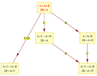
Figure 1: We propose to call $2B\rightarrow A\rightarrow A+B$ an ‘atom of multistationarity’; see Section 5.

1 Introduction

This work concerns an important class of dynamical systems arising in chemical engineering and systems biology, namely, chemical reaction systems. As bistable chemical systems are thought to be the underpinnings of biochemical switches, a key question is to determine which systems admit multiple steady states. In this work, we consider the question of whether the minimal (in a precise sense) networks, which we propose to call ‘atoms of multistationarity,’ characterize the entire set of multistationary networks. We prove that such atoms do characterize multistationarity for the case of fully open continuous-flow stirred-tank reactors (CFSTRs), which are networks in which all chemical species take part in the inflow and outflow (see Definition 2.4). For instance, the five networks depicted in Figure 1 are multistationary in the CFSTR setting, but only one is minimal with respect to ‘removing species’ (see Theorem 7.1). Following other analyses of small networks [13, 21, 22, 23, 24, 25], our main application is to those CFSTRs containing two non-flow reactions.

Chemical reaction systems are nonlinear and parametrized by unknown reaction rate constants. Thus, determining whether a chemical reaction network admits multiple steady states is difficult: for instance, in the mass-action kinetics setting, it requires determining existence of multiple positive solutions to a system of polynomials with unknown coefficients. However, various criteria have been developed that often can answer this question. For instance, the Deficiency, Advanced Deficiency, and Higher Deficiency Theories developed by Ellison, Feinberg, Horn, Jackson, and Ji in many cases can affirm that a network admits multiple steady states or can rule out the possibility [9, 11, 14, 15]. Similarly, the Jacobian Criterion and the more general injectivity test developed by Craciun and Feinberg can preclude multiple steady states [3, 4, 5, 6, 15, 17]. These results have been implemented in the CRN Toolbox, freely available computer software developed by Feinberg and improved by Ellison and Ji [10]. Related software programs include BioNetX [19, 20] and Chemical Reaction Network Software for Mathematica [18].

For systems for which the above software approaches are inconclusive, Conradi et al. advocate an approach which first determines whether certain subnetworks admit multiple positive steady states, and if so, tests whether these instances can be lifted to the original network [2]. Here, we too examine the topic of lifting multistationarity from a subnetwork to an overall network: Theorem 3.1, states that this can be accomplished as long as the steady states of interest are nondegenerate and the two networks share the same stoichiometric subspace. This result and its proof extend Theorem 2 in work of Craciun and Feinberg [4]. An important consequence of our theorem is that it provides the mathematical foundation for the technique of Siegal-Gaskins et al. which establishes bistability by way of ‘network ancestry’ (see Remark 3.3); their method was applied to a large class of simple gene regulatory networks [23].

A fully open continuous-flow stirred-tank reactor (CFSTR) is a network in which all chemical species enter the system at constant rates and are removed at rates proportional to their concentrations (see Definition 2.4). In the setting of these systems, we extend our results beyond subnetworks to ‘embedded networks’ which are obtained by removing species as well as reactions from a network (Definition 2.2). Corollary 4.6 states that if an embedded CFSTR of a CFSTR is multistationary then so is the CFSTR itself. Therefore, the set of multistationary CFSTRs is characterized by its minimal elements (with respect to the embedded network relation), and we pose the challenge of characterizing these atoms. In this work, we focus on cataloging the smallest atoms.

Recent work of the first author presented a simple characterization of the one-reaction fully open CFSTRs that admit multiple steady states in the mass-action kinetics setting (Theorem 2.11) [16]. Here we consider the bimolecular two-reaction CFSTRs; a network is ‘bimolecular’ if all of its chemical complexes contain at most two molecules. We enumerate all 386 reversible such networks. Of these, exactly 35 admit multiple positive steady states. Moreover, each admits a unique minimal multistationary sub-CFSTR, and these subnetworks form a poset with respect to the embedded network relation that has 11 minimal elements (Theorem 7.1). These 11 networks are precisely the CFSTR atoms of multistationarity in the bimolecular two-reaction setting. Note that a similar enumeration of small bimolecular networks was undertaken by Deckard, Bergmann, and Sauro [8], from which Pantea and Craciun sampled networks to compute the fraction of such networks that pass the Jacobian Criterion [20].

This article is organized as follows. Section 2 introduces chemical reaction systems. Our main result for lifting multiple steady states from subnetworks, Theorem 3.1, appears in Section 3. In Section 4, this result is extended in the case of fully open CFSTRs: Theorem 4.2 implies that steady states from embedded CFSTRs can be lifted as well. Section 5 introduces ‘atoms of multistationarity.’ Section 6 describes our approach to enumerating bimolecular two-reaction networks (Algorithm 6.4), and Section 7 determines which such networks are multistationary in the mass-action kinetics setting (Theorem 7.1) and displays the resulting atoms of multistationarity (Figure 3).

2 Chemical reaction network theory

In this section we review the standard notation and recall the classification of one-reaction CFSTRs.

2.1 Chemical reaction networks

We begin with an example of a chemical reaction:

$$2X_{1}+X_{2}~{}\rightarrow~{}X_{3}~{}.$$

Each $X_{i}$ is called a chemical species, and $2X_{1}+X_{2}$ and $X_{3}$ are called chemical complexes. Assigning the reactant complex $2X_{1}+X_{2}$ to the vector $y=(2,1,0)$ and the product complex $X_{3}$ to the vector $y^{\prime}=(0,0,1)$, we can write the reaction as $y\rightarrow y^{\prime}$. In general we let $s$ denote the total number of species $X_{i}$, and we consider a set of $r$ reactions, each denoted by

$$y_{k}\rightarrow y_{k}^{\prime}~{},$$

for $k\in\{1,2,\dots,r\}$, and $y_{k},y_{k}^{\prime}\in\mathbb{Z}^{s}_{\geq 0}$, with $y_{k}\neq y_{k}^{\prime}$. We index the entries of a complex vector $y_{k}$ by writing $y_{k}=\left(y_{k1},y_{k2},\dots,y_{ks}\right)\in\mathbb{Z}^{s}_{\geq 0}$, and we will call $y_{ki}$ the stoichiometric coefficient of species $i$ in complex $y_{k}$. For ease of notation, when there is no need for enumeration we typically will drop the subscript $k$ from the notation for the complexes and reactions.

Definition 2.1.

Let $\mathcal{S}=\{X_{i}\}$, $\mathcal{C}=\{y\},$ and $\mathcal{R}=\{y\to y^{\prime}\}$ denote finite sets of species, complexes, and reactions, respectively. The triple $\{\mathcal{S},\mathcal{C},\mathcal{R}\}$ is called a chemical reaction network if it satisfies the following:

1. for each complex $y\in\mathcal{C}$, there exists a reaction in $\mathcal{R}$ for which $y$ is the reactant complex or $y$ is the product complex, and

2. for each species $X_{i}\in\mathcal{S}$, there exists a complex $y\in\mathcal{C}$ that contains $X_{i}$.

A network decouples if there exist nonempty subsets $\mathcal{R}^{\prime}\subset\mathcal{R}$ and $\mathcal{R}^{\prime\prime}\subset\mathcal{R}$ such that $\mathcal{R}=\mathcal{R}^{\prime}~{}\dot{\cup}~{}\mathcal{R}^{\prime\prime}$ and such that the species involved in reactions in $\mathcal{R}^{\prime}$ are distinct from those of $\mathcal{R}^{\prime\prime}$. We next define a subnetwork and the more general concept of an ‘embedded’ network,’ which was introduced by the authors in [17, §4.2]. Informally, a network $N$ is an embedded network of a network $G$ if $N$ may be obtained from $G$ by removing reactions and ‘removing species.’

Definition 2.2.

Let $\mathfrak{G}=\{\mathcal{S},\mathcal{C},\mathcal{R}\}$ be a chemical reaction network.

1. Consider a subset of the species $S\subset\mathcal{S}$, a subset of the complexes $C\subset\mathcal{C}$, and a subset of the reactions $R\subset\mathcal{R}$.

   • The restriction of $R$ to $S$, denoted by $R|_{S}$, is the set of reactions obtained by taking the reactions in $R$ and removing all species not in $S$ from the reactant and product complexes. If a trivial reaction (one in which the reactant and product complexes are the same) is obtained in this process, then it is removed. Also removed are extra copies of repeated reactions.

   • The restriction of $C$ to $R$, denoted by $C|_{R}$, is the set of (reactant and product) complexes of the reactions in $R$.

   • The restriction of $S$ to $C$, denoted by $S|_{C}$, is the set of species that are in the complexes in $C$.

2. The network obtained from $\mathfrak{G}$ by removing a subset of species $\{X_{i}\}\subset\mathcal{S}$ is the network

   $$\left\{\mathcal{S}\setminus\{X_{i}\},~{}\mathcal{C}|_{\mathcal{R}|_{\mathcal{S}\setminus\{X_{i}\}}},~{}\mathcal{R}|_{\mathcal{S}\setminus\{X_{i}\}}\right\}~{}.$$

3. A subset of the reactions $\mathcal{R}^{\prime}\subset\mathcal{R}$ defines the subnetwork $\{\mathcal{S}|_{\mathcal{C}|_{\mathcal{R}^{\prime}}},\mathcal{C}|_{\mathcal{R}^{\prime}},\mathcal{R}^{\prime}\}$.

4. Let $\mathfrak{G}=\{\mathcal{S},\mathcal{C},\mathcal{R}\}$ be a chemical reaction network. An embedded network of $\mathfrak{G}$, which is defined by a subset of the species, $S=\left\{X_{i_{1}},X_{i_{2}},\dots,X_{i_{k}}\right\}\subset\mathcal{S}$, and a subset of the reactions, $R=\left\{R_{j_{1}},R_{j_{2}},\dots,R_{j_{l}}\right\}\subset\mathcal{R}$, that involve all species of $S$, is the network $(S,\mathcal{C}|_{R|_{S}},R|_{S})$ consisting of the reactions $R|_{S}$.

Remark 2.3.

We note that a network is also a subnetwork and an embedded network of itself. In fact, any subnetwork $\{\mathcal{S}|_{\mathcal{C}|_{\mathcal{R}^{\prime}}},\mathcal{C}|_{\mathcal{R}^{\prime}},\mathcal{R}^{\prime}\}$ is an embedded network, namely the one defined by the subset of species $\mathcal{S}|_{\mathcal{C}|_{\mathcal{R}^{\prime}}}$ and the subset of reactions $\mathcal{R}^{\prime}$.

We also note for readers who are familiar with species-reaction (SR) graphs that the definitions of ‘subnetwork’ and ‘embedded network’ can be interpreted as follows. Recall that the SR graph of a network consists of species vertices and reaction vertices, with edges arising from reactions in the network; for details, see [5]. A subnetwork corresponds to the subgraph of the SR graph induced by the full set of species and the subset of reaction vertices arising from reactions in the subnetwork. As for an embedded network, this arises as the subgraph induced by the corresponding subsets of species and reaction nodes.

One focus of our work is on CFSTRs, which we now define.

Definition 2.4.

1. A flow reaction contains only one molecule; such a reaction is either an inflow reaction $0\rightarrow X_{i}$ or an outflow reaction $X_{i}\rightarrow 0$.

2. A chemical reaction network is a continuous-flow stirred-tank reactor (CFSTR) if it contains all outflow reactions $X_{i}\rightarrow 0$ (for all $X_{i}\in\mathcal{S}$). A CFSTR is fully open if it additionally contains all inflow reactions $0\rightarrow X_{i}$. A sub-CFSTR is a subnetwork that is also a CFSTR.

We note that Craciun and Feinberg use the term ‘feed reactions’ for inflow reactions and ‘true reactions’ for non-flow reactions. In chemical engineering, a CFSTR refers to a well-mixed tank in which reactions occur. An inflow reaction represents the flow of species (at a constant rate) into the tank in which the non-flow reactions take place, and an outflow reaction represents the removal or degradation of a species (at rate proportional to its concentration).

Example 2.5.

Consider the following fully open CFSTR:

$$0\stackrel{{\scriptstyle[}}{{\kappa}}_{2}]{\kappa_{1}}{\rightleftarrows}A\quad\quad 0\stackrel{{\scriptstyle[}}{{\kappa}}_{4}]{\kappa_{3}}{\rightleftarrows}B\quad\quad 0\stackrel{{\scriptstyle[}}{{\kappa}}_{6}]{\kappa_{5}}{\rightleftarrows}C\quad\quad 2A\stackrel{{\scriptstyle[}}{{\kappa}}_{8}]{\kappa_{7}}{\rightleftarrows}A+B\stackrel{{\scriptstyle[}}{{\kappa}}_{10}]{\kappa_{9}}{\rightleftarrows}A+C~{}.$$ (1)

The following sub-CFSTR arises by removing two reactions:

$$0\stackrel{{\scriptstyle[}}{{\kappa}}_{2}=1]{\kappa_{1}}{\rightleftarrows}A\quad\quad 0\stackrel{{\scriptstyle[}}{{\kappa}}_{4}=1]{\kappa_{3}}{\rightleftarrows}B\quad\quad 0\stackrel{{\scriptstyle[}}{{\kappa}}_{6}=1]{\kappa_{5}}{\rightleftarrows}C\quad\quad 2A\stackrel{{\scriptstyle[}}{{\kappa}}_{8}]{~{}}{\leftarrow}A+B\stackrel{{\scriptstyle[}}{{\kappa}}_{10}]{~{}}{\leftarrow}A+C~{}.$$ (2)

Next, we obtain the following embedded network by removing species $C$:

$$0\stackrel{{\scriptstyle[}}{{\kappa}}_{2}=1]{\kappa_{1}}{\rightleftarrows}A\quad\quad 0\stackrel{{\scriptstyle[}}{{\kappa}}_{4}=1]{\kappa_{3}}{\rightleftarrows}B\quad\quad 2A\stackrel{{\scriptstyle[}}{{\kappa}}_{8}]{~{}}{\leftarrow}A+B\stackrel{{\scriptstyle[}}{{\kappa}}_{10}]{~{}}{\leftarrow}A~{}.$$ (3)

2.2 Dynamics and steady states

The concentration vector

$$x(t)=\left(x_{1}(t),x_{2}(t),\ldots,x_{|\mathcal{S}|}(t)\right)$$

will track the concentration $x_{i}(t)$ of the $i$-th species at time $t$. A chemical reaction network defines a dynamical system by way of a rate function for each reaction. In other words, to each reaction $y_{k}\to y_{k}^{\prime}$ we assign a smooth function $\displaystyle R_{k}(\cdot)=R_{y_{k}\to y_{k}^{\prime}}(\cdot)$ that satisfies the following assumption.

Assumption 2.6.

For $k\in\mathcal{R}$, $\displaystyle R_{k}(\cdot)=R_{y_{k}\to y_{k}^{\prime}}(\cdot):\mathbb{R}^{|\mathcal{S}|}_{\geq 0}\to\mathbb{R}$ satisfies:

1. $R_{y_{k}\to y_{k}^{\prime}}(\cdot)$ depends explicitly upon $x_{i}$ only if $\displaystyle y_{ki}\neq 0$.

2. $\displaystyle\frac{\partial}{\partial x_{i}}R_{y_{k}\to y_{k}^{\prime}}(x)\geq 0$ for those $x_{i}$ for which $\displaystyle y_{ki}\neq 0$, and equality can hold only if at least one coordinate of $x$ is zero.

3. $R_{y_{k}\to y_{k}^{\prime}}(x)=0$ if $x_{i}=0$ for some $i$ with $\displaystyle y_{ki}\neq 0$.

4. If $\displaystyle 1\leq y_{ki}<y_{\ell i}$, then $\displaystyle\lim_{x_{i}\to 0}\frac{R_{\ell}(x)}{R_{k}(x)}=0$, where all other $x_{j}>0$ are held fixed in the limit.

The final assumption simply states that if the $l$-th reaction demands strictly more molecules of species $X_{i}$ as inputs than does the $k$-th reaction, then the rate of the $l$-th reaction decreases to zero faster than the $k$-th reaction, as $x_{i}\to 0$. The functions $R_{k}$ are called the kinetics of the system.

Definition 2.7.

Consider a chemical reaction network $\left\{\mathcal{S},\mathcal{C},\mathcal{R}=\{y_{k}\rightarrow y_{k}^{\prime}\}\right\}$ and a choice of kinetics $\{R_{k}\}$ that satisfy Assumption 2.6.

1. The following system of ODEs defines a dynamical system is called a chemical reaction system:

   $$\dot{x}(t)\quad=\quad\sum_{k=1}^{\mathcal{R}}R_{k}(x(t))(y_{k}^{\prime}-y_{k})\quad=:\quad f(x(t))~{},$$ (4)

   where the second equality is a definition.

2. The stoichiometric subspace of the network is the span of all reaction vectors $y_{k}^{\prime}-y_{k}$. We will denote this space by $S$ and its dimension by $\sigma$:

   $$S\quad:=\quad{\rm span}\left\{y_{1}^{\prime}-y_{1},~{}y_{2}^{\prime}-y_{2},~{}\dots~{},~{}y_{|\mathcal{R}|}^{\prime}-y_{|\mathcal{R}|}\right\}~{}\subset~{}\mathbb{R}^{|\mathcal{S}|}~{}.$$

   Note that (4) implies that a trajectory $x(t)$ that begins at a positive vector $x(0)=c^{0}\in\mathbb{R}^{s}_{>0}$ remains in the stoichiometric compatibility class, which we denote by

   $$\mathcal{P}\quad:=\quad(c^{0}+S)\cap\mathbb{R}^{|\mathcal{S}|}_{\geq 0}~{},$$ (5)

   for all positive time; in other words, this set $\mathcal{P}$ is forward-invariant with respect to (4). Two points in the same stoichiometric compatibility class $\mathcal{P}$ are said to be stoichiometrically compatible.

3. A concentration vector $\overline{x}\in\mathbb{R}^{|\mathcal{S}|}_{>0}$ is a (positive) steady state of the system (4) if $f(\overline{x})=\overline{0}$. A steady state $\overline{x}$ is nondegenerate if $\operatorname{Im}df(\overline{x})=S$. (Here, “$df(\overline{x})$” is the Jacobian matrix of $f$ at $\overline{x}$: the ${|\mathcal{S}|}\times{|\mathcal{S}|}$-matrix whose $(i,j)$-th entry is equal to the partial derivative $\frac{\partial f_{i}}{\partial x_{j}}(\overline{x})$). A nondegenerate steady state $\overline{x}$ is exponentially stable if each of the $\sigma:=\dim S$ nonzero eigenvalues of $df(\overline{x})$ (viewed over the complex numbers) has negative real part.

In the case of a CFSTR, the reaction vector for the $i$-th inflow reaction is the $i$-th canonical basis vector of $\mathbb{R}^{|\mathcal{S}|}$, so the stoichiometric subspace is $S=\mathbb{R}^{|\mathcal{S}|}$. It follows that for a CFSTR, the unique stoichiometric compatibility class is the nonnegative orthant: $\mathcal{P}=\mathbb{R}^{|\mathcal{S}|}_{\geq 0}$.

An important example of kinetics is mass-action kinetics; a chemical reaction system is said to have mass-action kinetics if all rate functions $R_{k}$ take the following multiplicative form:

$$R_{k}(x)\quad=\quad\kappa_{k}x_{1}^{y_{k1}}x_{2}^{y_{k2}}\cdots x_{|\mathcal{S}|}^{y_{k{|\mathcal{S}|}}}\quad=:\quad\kappa_{k}x^{y_{k}}~{},$$ (6)

for some vector of positive reaction rate constants $(\kappa_{1},\kappa_{2},\dots,\kappa_{|\mathcal{R}|})\in\mathbb{R}_{>0}^{|\mathcal{R}|}$, with the convention that $0^{0}=1$. It is easily verified that each $R_{k}$ defined via (6) satisfies Assumption 2.6. Combining (4) and (6) gives the following system of mass-action ODEs:

$$\dot{x}(t)\quad=\quad\sum_{k=1}^{|\mathcal{R}|}\kappa_{k}x(t)^{y_{k}}(y_{k}^{\prime}-y_{k})\quad=:\quad f(x(t))~{}.$$ (7)

In the following example and all others in this work, we will label species by distinct letters such as $A,B,\dots$ rather than $X_{1},X_{2},\dots$.

Example 2.8.

We now return to the CFSTR (1) in Example 2.5. The mass-action differential equations (7) for this network are the following:

$$\frac{d{x_{A}}}{dt}\quad =\quad{\kappa_{1}}-\kappa_{2}{x_{A}}-\kappa_{7}x_{A}^{2}+{\kappa_{8}}{x_{A}x_{B}}$$

$$\frac{dx_{B}}{dt}\quad =\quad{\kappa_{3}}-\kappa_{4}{x_{B}}+\kappa_{7}x_{A}^{2}-{\kappa_{8}}{x_{A}x_{B}}-\kappa_{9}x_{A}x_{B}+{\kappa_{10}}{x_{A}x_{C}}$$ (8)

$$\frac{dx_{C}}{dt}\quad =\quad{\kappa_{5}}-\kappa_{6}{x_{C}}+\kappa_{9}x_{A}x_{B}-{\kappa_{10}}{x_{A}x_{C}}~{}.$$

Note that a chemical reaction network gives rise to a family of mass-action kinetics systems parametrized by a choice of one reaction rate constant $\kappa_{k}\in\mathbb{R}_{>0}$ for each reaction, and all reactions not in the network can be viewed as having reaction rate constant equal to zero. We now generalize this concept of a parametrized family for other kinetics.

Definition 2.9.

1. A parametrized family of kinetics $\mathcal{K}$ for chemical reaction networks on $|\mathcal{S}|$ species is an assignment to each possible reaction $y_{k}\to y_{k}^{\prime}$ (that involves only species from $\mathcal{S}$) a smooth function

   $$\mathbb{R}_{\geq 0}\times\mathbb{R}_{\geq 0}^{\mathcal{S}} \to\mathbb{R}^{\mathcal{S}}$$

   $$(\kappa_{k},x) \mapsto R_{k}^{\kappa_{k}}(x)$$

   such that

   • for $\kappa_{k}>0$, the function $R_{k}^{\kappa_{k}}(x)$ is a rate function for the reaction $y_{k}\to y_{k}^{\prime}$ that satisfies Assumption 2.6, and

   • when $\kappa_{k}=0$, then $R_{k}^{\kappa_{k}}(x)$ is the zero function.

2. Let $\mathfrak{G}$ be a chemical reaction network, and let $\mathcal{K}$ be a parametrized family of kinetics on $|\mathcal{S}|$ species. Then $\mathfrak{G}$ is said to admit multiple $\mathcal{K}$ steady states or is $\mathcal{K}$-multistationary if there exist kinetics $\{R^{\kappa_{k}}_{k}\}$ arising from $\mathcal{K}$ and a stoichiometric compatibility class $\mathcal{P}$ such that the resulting system (4) has two or more positive steady states in $\mathcal{P}$. Moreover, such a network is said to admit bistability if such steady states can be found that are stable.

As noted above, an important family of kinetics $\mathcal{K}$ is that of mass-action kinetics; in this case, $\mathfrak{G}$ admits multiple mass-action steady states if there exist rate constants $\kappa_{k}\in\mathbb{R}_{>0}$ and a stoichiometric compatibility class $\mathcal{P}$ such that the mass-action system (7) admits at least two positive steady states in $\mathcal{P}$.

Example 2.10.

We again consider the CFSTR (1) examined in Examples 2.5 and 2.8. Recall that for a CFSTR, the unique stoichiometric compatibility class is the nonnegative orthant: here, $\mathcal{P}=\mathbb{R}^{3}_{\geq 0}$. Therefore, our CFSTR (1) admits multiple positive mass-action steady states if and only if there exist reaction rate constants $\kappa_{1},\kappa_{2},\dots,\kappa_{10}\in\mathbb{R}_{>0}$ such that the differential equations (2.8) have at least two positive steady states. Indeed, the CRN Toolbox [10] determines that when the mass-action system takes the following rate constants:

$$\left(\kappa_{1},\kappa_{2},\kappa_{3},\kappa_{4},\kappa_{5},\kappa_{6},\kappa_{7},\kappa_{8},\kappa_{9},\kappa_{10}\right)\quad=\quad$$

$$\quad(1,1,1,1,41774.858,1,2.5081*10^{-4},7.3335*10^{-3},1.1614*10^{-4},7.5610*10^{-5})~{},$$

there are two steady states:

$$x^{*}\quad =\quad(63.143335,136.35902,41577.356)\quad\quad{\rm and}$$

$$x^{**}\quad =\quad(25473.839,1007.5644,15295.454)~{}.$$

2.3 Classification of multistationary one-reaction CFSTRs

We now recall the following theorem, due to the first author:

Theorem 2.11 ([16]).

1. Consider a CFSTR which contains only one non-flow reaction:

   $$a_{1}X_{1}+a_{2}X_{2}+\cdots+a_{s}X_{s}\quad\rightarrow\quad b_{1}X_{1}+b_{2}X_{2}+\cdots+b_{s}X_{s}~{},$$

   where $a_{i},b_{i}\geq 0$. Then the CFSTR admits multiple positive mass-action steady states if and only if $\sum_{i:~{}b_{i}>a_{i}}a_{i}>1$. Moreover, these multistationary CFSTRs admit nondegenerate steady states.

2. Consider a CFSTR in which the only non-flow reactions consist of a pair of reversible reactions:

   $$a_{1}X_{1}+a_{2}X_{2}+\cdots+a_{s}X_{s}\quad\leftrightarrows\quad b_{1}X_{1}+b_{2}X_{2}+\cdots+b_{s}X_{s}~{},$$

   where $a_{i},b_{i}\geq 0$. The CFSTR admits multiple positive mass-action steady states if and only if the following holds:

   $$\sum_{i:~{}b_{i}>a_{i}}a_{i}>1\quad{\rm or}\quad\sum_{i:~{}a_{i}>b_{i}}b_{i}>1~{}.$$

   Moreover, these multistationary CFSTRs admit nondegenerate steady states.

The current work was motivated by the question of whether a similar theorem exists for the class of CFSTRs that consists of networks with two reversible nonflow reactions and their sub-CFSTRs.

3 Lifting multistationarity from subnetworks

Consider the following question: if a subnetwork $N$ of a network $G$ admits multiple positive steady states, then does $G$ as well? Theorem 3.1 asserts that the answer to this question is ‘yes,’ provided that the steady states are nondegenerate and the two networks share the same stoichiometric subspace (note that the stoichiometric subspace of $N$ is always contained in that of $G$). The proof lifts each steady state $x^{*}$ of $N$ to a nearby steady state of $G$.

Theorem 3.1.

Let $N$ be a subnetwork of a chemical reaction network $G$ such that they have the same stoichiometric subspace: $S_{N}=S_{G}$. Let $\mathcal{K}$ be a parametrized family of kinetics on the species of $G$. Then the following holds:

• If $N$ admits multiple nondegenerate positive $\mathcal{K}$ steady states, then $G$ does as well. Additionally, if $N$ admits finitely many such steady states, then $G$ admits at least as many.

• Moreover, if $N$ admits multiple positive exponentially stable steady states, then $G$ does as well. Additionally, if $N$ admits finitely many such steady states, then $G$ admits at least as many.

We note that our theorem is similar to Theorem 2 in work of Craciun and Feinberg [4]; their theorem allows multiple steady states to be lifted from an ‘entrapped species’ network (that is, only certain species are in the outflow) to the corresponding ‘fully diffusive’ network (all species are in the outflow). In addition, their theorem is stated as a contrapositive version of ours. Our proof of Theorem 3.1 makes use of the following homotopy theory result, which is a modified form of Theorem 1.1 in Craciun, Helton, and Williams [7].

Lemma 3.2.

Let $S\subset\mathbb{R}^{n}$ be a vector subspace, let $\mathcal{P}\subset\mathbb{R}^{n}$ be a polyhedron contained in an affine translation of $S$, and let $\Omega\subset\operatorname{int}(\mathcal{P})$ be a bounded domain in the relative interior of $\mathcal{P}$. Assume that $g_{\lambda}:\overline{\Omega}\to S$, for $\lambda\in[0,1]$, is a continuously-varying family of smooth functions such that

1. for all $\lambda\in[0,1]$, $g_{\lambda}$ has no zeroes on the boundary of $\Omega$, and

2. for $\lambda=0$ and $\lambda=1$, $\operatorname{Im}dg_{\lambda}(\overline{x})=S$ for all $x\in\Omega$.

Then the number of zeroes of $g_{0}$ in $\Omega$ equals the number of zeroes of $g_{1}$ in $\Omega$.

We now prove Theorem 3.1.

Proof of Theorem 3.1.

First, note that the network $G$ and its subnetwork $N$ must have the same set of species $\mathcal{S}$ in order for their stoichiometric subspaces to coincide. We let $S$ denote the shared stoichiometric subspace: $S:=S_{G}=S_{N}$. Now, let $\mathcal{R}^{\prime}$ denote the set of reactions of $G$ that are not in $N$: $\mathcal{R}_{G}\quad=\quad\mathcal{R}_{N}~{}\dot{\cup}~{}\mathcal{R}^{\prime}$. We now assume that the subnetwork $N$ admits multiple nondegenerate positive steady states; that is, there exist rate constants $\kappa_{1}^{*},\kappa_{2}^{*},\dots,\kappa_{|\mathcal{R}_{N}|}^{*}\in\mathbb{R}_{>0}$ such that there exist distinct, stoichiometrically compatible, nondegenerate positive steady states $x^{*}$ and $x^{**}$ of the chemical reaction system $(N,\kappa_{i}^{*})$ arising from $\mathcal{K}$. Write $f_{N}$ for the differential equations of $(N,\kappa_{i}^{*})$. Now $x^{*}$ is a nondegenerate steady state, so there exists a relatively open ball $\Omega$ around $x^{*}$ in the interior of $\mathcal{P}$ such that (1) $x^{*}$ is the unique steady state (zero of $f_{N}$) in $\Omega$, and (2) $\operatorname{Im}df_{N}(x)=S$ for all $x\in\Omega$. Note that (2) can be accomplished because the non-vanishing of a determinant is an open condition and because the matrix $df_{N}(x)$ varies continuously in $x$.

For any vector of reaction parameters $\kappa\in\mathbb{R}_{>0}^{|\mathcal{R}^{\prime}|}$, we define the following the following family of functions for $0\leq\lambda\leq 1$:

$$g^{\kappa}_{\lambda}(x):=f_{N}(x)+\sum_{k\in\mathcal{R}^{\prime}}(y_{k}^{\prime}-y_{k})R^{\lambda\kappa_{k}}_{k}(x)~{}.$$

It follows that $g^{\kappa}_{\lambda}(x)$ gives the differential equations (4) of the chemical reaction system arising from the network $G$ and the following reaction parameters with respect to the kinetics $\mathcal{K}$:

$$(\kappa^{*},\kappa)\quad:=\quad\left(\kappa_{1}^{*},\kappa_{2}^{*},\dots,\kappa_{|\mathcal{R}_{N}|}^{*},\lambda\kappa_{1},\lambda\kappa_{2},\dots,\lambda\kappa_{|\mathcal{R}^{\prime}|}\right)\in\mathbb{R}_{>0}^{|\mathcal{R}_{G}|}~{}.$$ (9)

Note that $g^{\kappa}_{0}(x)=f_{N}(x)$. Next, by continuity in $\kappa$ and the compactness of the boundary of $\Omega$, there exists a vector of reaction parameters $\kappa^{\dagger}\in\mathbb{R}_{>0}^{|\mathcal{R}^{\prime}|}$ such that for all $0\leq\lambda$, the function $g^{\kappa^{\dagger}}_{\lambda}(x)$ has no zeroes on the boundary of $\Omega$. By continuity in $\lambda$, and by scaling $\kappa^{\dagger}$ smaller if necessary, we may assume additionally that $\operatorname{Im}d_{x}g^{\kappa^{\dagger}}_{\lambda}(x)=S$ for all $x\in\Omega$. Therefore, Lemma 3.2 allows us to conclude that the chemical reaction system $\left(G,(\kappa^{*},\lambda\kappa^{\dagger})\right)$ has a nondegenerate steady state in the ball $\Omega$ for all $0\leq\lambda\leq 1$.

We now complete the proof by repeating the argument with $\widetilde{x}^{**}$, taking care that the ball around $\widetilde{x}^{**}$ does not intersect that of $\widetilde{x}^{*}$; we replace $\kappa^{\dagger}$ by a scaled-down version ($\mu\kappa^{\dagger}$ for some $0<\mu<1$) if necessary. It follows that $\left(G,(\kappa^{*},\lambda\kappa^{\dagger})\right)$ has at least two nondegenerate steady states. The case of three or more nondegenerate steady states generalizes in a straightforward way. For the stability result, we simply note that the eigenvalues of a matrix vary continuously under continuous perturbations (in this case, arising from the parameter $\lambda$). ∎

Remark 3.3.

One application of Theorem 3.1 is that it provides the mathematical justification for the technique of Siegal-Gaskins et al. which establishes bistability in the mass-action setting by way of ‘network ancestry’ [23]. In their examination of $40,680$ small gene regulatory networks, $14,721$ initially were established to be bistable by the implementation of Advanced Deficiency Theory in the CRN Toolbox [10], and an additional $22,050$ were classified as bistable by virtue of containing one of the $14,721$ bistable networks as a subnetwork (‘ancestor’) such that both networks have the same stoichiometric subspace. A similar approach is taken by Conradi et al. for lifting multiple steady states from certain subnetworks called ‘elementary flux modes’ [2]. We note that their criterion for lifting steady states does not require that the stoichiometric subspaces of the network and its subnetwork to coincide [2, Supporting Information].

The next example illustrates why the hypothesis of nondegeneracy is required in Theorem 3.1. A larger such example appears in the work of Craciun and Feinberg [4, §6].

Example 3.4.

Consider the following (non-CFSTR) network:

(10)

The CRN Toolbox [10] determines that network (10) does not admit multiple positive mass-action steady states, but the following subnetwork does admit multiple degenerate positive steady states:

$$A\stackrel{{\scriptstyle[}}{{~{}}}]{\kappa_{1}}{\leftarrow}B\stackrel{{\scriptstyle[}}{{~{}}}]{\kappa_{2}}{\rightarrow}C\quad\quad A+C\stackrel{{\scriptstyle[}}{{~{}}}]{\kappa_{3}}{\rightarrow}2B~{}.$$ (11)

In fact, it is straightforward to verify that steady states exist for network (11) if and only if $\kappa_{1}=\kappa_{2}$, and in this case, each two-dimensional compatibility class contains an infinite one-dimensional set of degenerate steady states.

One way for a network and its subnetwork to share the same stoichiometric subspace is for the subnetwork to be obtained by making some reversible reactions irreversible. Thus, Theorem 3.1 yields the following corollary.

Corollary 3.5.

For a chemical reaction network $N$, let $\mathcal{K}$ be a parametrized family of kinetics on the species of $N$. Let $G$ be a network obtained from $N$ by making some irreversible reactions of $N$ reversible. Then if $N$ admits multiple nondegenerate positive $\mathcal{K}$ steady states, then $G$ does as well.

The next corollary states that Theorem 3.1 allows multiple positive steady states to be lifted from a sub-CFSTR to a fully open CFSTR. Therefore, the set of minimal multistationary CFSTRs (with respect to the subnetwork relation) completely defines the set of all fully open multistationary CFSTRs: a fully open CFSTR admits multiple steady states if and only if it contains as a subnetwork one of these minimal CFSTRs. This result will be useful in our classification of small multistationary CFSTRs in Section 7.

Corollary 3.6.

Let $N$ be a sub-CFSTR of a fully open CFSTR $G$, and let $\mathcal{K}$ be a parametrized family of kinetics on the species of $G$. Then, if $N$ admits multiple nondegenerate positive $\mathcal{K}$ steady states, then $G$ does as well.

Proof.

Assume that the species of $N$ are $X_{1},X_{2},\dots,X_{s_{1}}$ and the species of $G$ are $X_{1},X_{2},\dots,$ $X_{s_{1}+s_{2}}$. Let $N^{\prime}$ be the CFSTR obtained from $N$ by appending the flow reactions $0\leftrightarrows X_{s_{1}+1}$, $0\leftrightarrows X_{s_{1}+2}$, …, $0\leftrightarrows X_{s_{1}+s_{2}}$ for all species of $G$ that are not in $N$. Clearly, $N^{\prime}$ is a subnetwork of $G$, and they share the same stoichiometric subspace, namely, $\mathbb{R}^{s_{1}+s_{2}}$. By applying Theorem 3.1 to $N^{\prime}$ and $G$, we see that if $N^{\prime}$ admits multiple nondegenerate positive steady states, then $G$ does as well. Therefore, it remains only to show that $N$ admits multiple nondegenerate positive steady states if and only if $N^{\prime}$ does.

Consider any outflow rate parameter $\kappa_{s_{1}+i}^{\rm out}>0$ for one of the new outflow reactions. Then by Assumption 2.6, the rate function $R_{\kappa_{s_{1}+i}^{\rm out}}^{X_{s_{1}+i}\to 0}(x)$ depends only on $x_{s_{1}+i}$ and is increasing in $x_{s_{1}+i}$ from

$$0=R_{\kappa_{s_{1}+i}^{\rm out}}^{X_{s_{1}+i}\to 0}(x_{1},\dots,x_{s_{1}+i-1},0,x_{s_{1}+i+1},\dots x_{s_{1}+s_{2}})~{}.$$

As for the corresponding inflow rate function, Assumption 2.6 implies that $R_{\kappa_{s_{1}+i}^{\rm in}}^{0\to X_{s_{1}+i}}(x)$ is a positive constant function, and this constant depends only on the parameter ${\kappa_{s_{1}+i}^{\rm in}}$ and is in fact increasing in this parameter for sufficiently small values, with $R_{0}^{0\to X_{s_{1}+i}}(x)=0$. Thus, we can choose a sufficiently small inflow parameter ${\kappa_{s_{1}+i}^{\rm in}}>0$ such that there exists a positive value $x^{*}_{s_{1}+i}>0$ for which the rate functions are equal at $x$ when $x_{s_{1}+i}=x^{*}_{s_{1}+i}$.

Therefore, it follows that $x^{*}=\left(x^{*}_{1},x^{*}_{2},\dots,x^{*}_{s_{1}}\right)\in\mathbb{R}_{>0}^{s_{1}}$ is a nondegenerate positive steady state of the system $\left(N,(\kappa_{1},\kappa_{2},\dots,\kappa_{|\mathcal{R}_{N}|})\right)$ if and only if the concentration vector

$$\left(x^{*}_{1},x^{*}_{2},\dots,x^{*}_{s_{1}},x^{*}_{s_{1}+1},\dots,x^{*}_{s_{1}+s_{2}}\right)\in\mathbb{R}_{>0}^{s_{1}+s_{2}}$$

is a nondegenerate positive steady state of the system

$$\left(N^{\prime},(\kappa_{1},\kappa_{2},\dots,\kappa_{|\mathcal{R}_{N}|},\kappa_{s_{1}+1}^{\rm in},\kappa_{s_{1}+1}^{\rm out}\dots,\kappa_{s_{1}+s_{2}}^{\rm out})\right)~{},$$

where the rates $\kappa_{s_{1}+i}^{\rm in}$ and $\kappa_{s_{1}+i}^{\rm out}$ are chosen as described above. This completes the proof. ∎

4 Lifting mass-action multistationarity from embedded CFSTRs

Corollary 3.6 stated that multistationarity can be lifted from sub-CFSTRs; in this section, we generalize the result to the case of embedded CFSTRs in the mass-action setting (Corollary 4.6).

We first need the following generalization of inflow/outflow reactions in order to allow for reactions such as $A\leftrightarrows 2A$ which also have a mass-action steady state at $\overline{x_{A}}=1$ when the two reaction rate constants are equal.

Definition 4.1.

A mass-action flow-type subnetwork for a species $X_{i}$ of a chemical reaction network $G$ is a nonempty subnetwork $N$ of $G$ such that

1. the reactions in $N$ involve only species $X_{i}$, and

2. there exists a choice of reaction rate constants $\kappa_{r}^{*}$ for the reactions $r\in\mathcal{R}_{N}$ of $N$ such that for the resulting mass-action system of this subnetwork $N$, $\overline{x_{i}}=1$ is a nondegenerate steady state.

The following theorem is analogous to Theorem 3.1.

Theorem 4.2.

Let $N$ be an embedded network of a network $G$ such that

1. the stoichiometric subspace of $N$ is full-dimensional: $S_{N}=\mathbb{R}^{|\mathcal{S}_{N}|}$, and

2. for each species $X_{i}$ that is in $G$ but not in $N$, there exists a mass-action flow-type subnetwork of $G$ for $X_{i}$.

Then the following holds:

• If $N$ admits multiple nondegenerate positive mass-action steady states, then $G$ does as well. Additionally, if $N$ admits finitely many such steady states, then $G$ admits at least as many.

• Moreover, if $N$ admits multiple positive exponentially stable mass-action steady states, then $G$ does as well. Additionally, if $N$ admits finitely many such steady states, then $G$ admits at least as many.

The proof of Theorem 4.2 requires the following lemma, which states that for certain simple embedded networks obtained by removing only one species, each nondegenerate steady state $u$ can be lifted to a steady state of the larger network that is near $(u,1)$.

Lemma 4.3.

Let $G$ be a chemical reaction network with $s$ species denoted by $X_{1},X_{2},\dots,X_{s}$, and let $N$ be an embedded network of $G$ with $s-1$ species $X_{1},X_{2},\dots,X_{s-1}$ such that $N$ is full-dimensional: $S_{N}=\mathbb{R}^{s-1}$. Assume that the reactions of $G$ and the reactions of $N$ can be written as, respectively, $\mathcal{R}_{G}=\{\widetilde{R_{1}},\widetilde{R_{2}},\dots,\widetilde{R_{m}},R_{m+1},\dots,R_{m+n}\}$ and $\mathcal{R}_{N}=\{R_{1},R_{2},\dots,R_{m}\}$ such that:

1. for $i=1,2,\dots,m$, the reaction $R_{i}$ of $N$ is obtained from the corresponding reaction $\widetilde{R_{i}}$ of $G$ by removing species $X_{s}$, and

2. all remaining reactions of $G$, namely $\{R_{m+1},R_{m+2},\dots,R_{m+n}\}$, together form a mass-action flow-type subnetwork for the species $X_{s}$.

For a choice of rate constants $\kappa^{*}_{1},\kappa^{*}_{2},\dots,\kappa^{*}_{m}>0$, let $\Sigma\left(N,\{\kappa^{*}_{1},\kappa^{*}_{2},\dots,\kappa^{*}_{m}\}\right)$ denote a finite set of nondegenerate positive mass-action steady states of the system arising from $N$ and the $\kappa^{*}_{i}$. Then for sufficiently small $\epsilon>0$, there exist reaction rate constants $\kappa^{*}_{m+1},\kappa^{*}_{m+2},\dots,\kappa^{*}_{m+n}$ for the flow-type subnetwork of $G$ such that for all $u\in\Sigma\left(N,\{\kappa^{*}_{1},\kappa^{*}_{2},\dots,\kappa^{*}_{m}\}\right)$, there exists a nondegenerate positive mass-action steady state $\widetilde{u}$ of the system arising from $G$ and $\kappa^{*}_{1},\kappa^{*}_{2},\dots,\kappa^{*}_{m+n}$ with $|\widetilde{u}-(u,1)|<\epsilon$. Additionally, if $u$ is exponentially stable, then $\widetilde{u}$ is as well.

Proof.

Fix a choice of reaction rate constants $\kappa^{*}_{1},\kappa^{*}_{2},\dots,\kappa^{*}_{m}$, and let $\Sigma:=\Sigma\left(N,\{\kappa^{*}_{1},\kappa^{*}_{2},\dots,\kappa^{*}_{m}\}\right)$ be as in the statement of the lemma.

We view $G=\widetilde{N}\dot{\cup}M$ as the disjoint union of two subnetworks, one which consists of the reactions $\widetilde{R_{1}},\widetilde{R_{2}},\dots,\widetilde{R_{m}}$, which we denote by $\widetilde{N}$, and the second which consists of $R_{m+1},R_{m+2},\dots,$ $R_{m+n}$, which we denote by $M$. As $M$ is a mass-action flow-type subnetwork for the species $X_{s}$, there exist rate constants $\overline{\kappa_{m+1}},\overline{\kappa_{m+2}},\dots,\overline{\kappa_{m+n}}>0$ such that the resulting mass-action ODE system, denoted by $f_{M}(x_{s})$, has a nondegenerate steady state at $\overline{x_{s}}=1$.

Next, we denote by $f_{\widetilde{N}}(x)$ the mass-action ODE system (7) arising from the subnetwork $\widetilde{N}$ and the fixed rate constants $\kappa^{*}_{1},\kappa^{*}_{2},\dots,\kappa^{*}_{m}$. Consider the following map from $\mathbb{R}_{\geq 0}\times\mathbb{R}_{\geq 0}^{s}$ to $\mathbb{R}^{s}$:

$$f_{G}(k,x):=\left(f_{\widetilde{N},1}(x),~{}f_{\widetilde{N},2}(x),~{}\dots~{},f_{\widetilde{N},s-1}(x),~{}f_{\widetilde{N},s}(x)+kf_{M}(x_{s})\right)~{}.$$ (12)

(Note that $f_{\widetilde{N},i}$ denotes the $i$-th coordinate function of $f_{\widetilde{N}}$.) It follows that $f_{G}(k,x)$ denotes the mass-action ODEs for the network $G$ with respect to the rate constants

$$\kappa_{1}^{*},\kappa_{2}^{*},\dots,\kappa_{m}^{*},k\overline{\kappa_{m+1}},k\overline{\kappa_{m+2}},\dots k\overline{\kappa_{m+n}}~{}.$$

We scale the last coordinate of $f_{G}(k,x)$ by $1/{k}$ and make the substitution $\delta=1/k$ to obtain:

$$F_{G}(\delta,x): =\left(f_{\widetilde{N},1}(x),~{}\dots~{},f_{\widetilde{N},s-1}(x),~{}f_{M}(x_{s})\right)+\left(0,\dots,0,\delta f_{\widetilde{N},s}(x)\right)$$ (13)

$$=:h(x)+\delta\left(0,\dots,0,f_{\widetilde{N},s}(x)\right)~{},$$

where $h(x)$ is defined by the second equality. Hence, it suffices to prove that for sufficiently small $\epsilon>0$ and for all $u\in\Sigma$, there exists a $\delta>0$ such that there exists a nondegenerate zero $\widetilde{u}$ of $F_{G}(\delta,x)$ with $|\widetilde{u}-(u,1)|<\epsilon$.

Fix $u\in\Sigma$. We now claim that $h$ has a nondegenerate zero at $(u,1)$. The final coordinate of $h$ satisfies $h_{s}(u,1)=f_{M}(1)=0$ by construction. As for the remaining coordinates $i=1,2,\dots,s-1$, we compute

$$h_{i}(u,1)=f_{\widetilde{N},i}(u,1)=f_{N}(u)=0~{}.$$ (14)

We now explain the second equality in (14). When the reaction $\widetilde{R_{j}}$ in $\widetilde{N}$ is $\widetilde{y_{j}}\rightarrow\widetilde{y_{j}^{\prime}}$ then the reaction $R_{j}$, given by $y_{j}\to y_{j}^{\prime}$, is such that the projection of $\widetilde{y_{j}}$ onto the first $s-1$ coordinates is $y_{j}$ and similarly for $\widetilde{y_{j}^{\prime}}$. Thus, the reaction vector $\widetilde{y_{j}^{\prime}}-\widetilde{y_{j}}$ projects to $y_{j}^{\prime}-y_{j}$ and $(u_{1},u_{2},\dots,u_{s-1},1)^{\widetilde{y_{j}}}=(u_{1},u_{2},\dots,u_{s-1})^{y_{j}}$. Finally, $(u,1)$ is nondegenerate, because $dh(u,1)$ is an $s\times s$-matrix in which the upper-left $(s-1)\times(s-1)$-submatrix is the nonsingular matrix $df_{N}(u)$ and the bottom row is $(0,0,\dots,0,\frac{df_{M}}{dx_{s}}(1))$ with $\frac{df_{M}}{dx_{s}}(1)\neq 0$ by hypothesis.

As $(u,1)$ is nondegenerate, there exists a constant $\epsilon(u)>0$ such that the resulting $\epsilon(u)$-neighborhood of $(u,1)$, which we denote by $\Omega$, is such that (1) $\Omega$ is in the positive orthant $\mathbb{R}_{>0}^{s}$, (2) $(u,1)$ is the unique zero of $h$ in $\Omega$, and (3) $dh(x)$ is nonsingular for all $x\in\Omega$. Consider again the function $F_{G}(\delta,x)$ defined in (13), and note that $F(0,x)=h(x)$. By continuity in $\delta$ and the compactness of the boundary of $\Omega$, there exists $\delta(u)>0$ such that for all $0\leq\delta\leq\delta(u)$, the function $F_{G}(\delta,x)$ has no zeroes on the boundary of $\Omega$. Again by continuity and by decreasing $\delta(u)$ if necessary, we may assume that $dF(\delta,x)$ (the matrix of partial derivatives with respect to the $x_{1},x_{2},\dots,x_{s}$) is nonsingular for all $0\leq\delta\leq\delta(u)$ and for all $x\in\Omega$. Therefore, Lemma 3.2 allows us to conclude that $F_{G}(\delta,x)$ has a unique nondegenerate zero $\widetilde{u}$ in $\Omega$ (that is, $|\widetilde{u}-(u,1)|<\epsilon(u)$) for all $0\leq\delta\leq\delta(u)$.

Now let $\epsilon^{*}$ be the minimum of all such $\epsilon(u)$, where $u\in\Sigma$. Additionally, we decrease $\epsilon^{*}$ if necessary so that the resulting $\epsilon$-neighborhoods of the points $u$ do not intersect. The lemma now follows with the $\epsilon^{*}$ as a cut-off: given any $0<\epsilon<\epsilon^{*}$, the above arguments for each $u$ can be made using $\epsilon$ in place of $\epsilon(u)$. Taking the minimum, denoted by $\delta^{*}$, of the resulting cut-offs $\delta(u)$, we obtain nondegenerate zero $\widetilde{u}$ of $F_{G}(\delta^{*},x)$ such that $|\widetilde{u}-(u,1)|<\epsilon$.

For the stability result, the eigenvalues of a matrix vary continuously under continuous perturbations (in this case, arising from the parameter $\delta$). ∎

Remark 4.4.

In the proof of Lemma 4.3, the $s$-dimensional dynamical system (12) may be represented by

$$\dot{x}=f_{\widetilde{N}}(x)+kg_{M}(x_{s})~{},$$

where $g_{M}(x_{s}):=(0,\ldots,0,f_{M}(x_{s}))$. When $k$ is sufficiently large and $x_{s}$ is in the domain of attraction of $\overline{x_{s}}=1$ with $\lvert g_{M}(x_{s})\rvert\sim O(1)$, then $\dot{x}\sim kg_{M}(x_{s})$, which has dynamics close to the one-dimensional system $\dot{x}_{s}=kf_{M}(x_{s})$. However, when $x_{s}$ is close to $\overline{x_{s}}=1$ with $\lvert g_{M}(x_{s})\rvert\sim O(1/k^{2})$, then $\dot{x}\sim f_{\widetilde{N}}(x)$, the dynamics of which are effectively those of an $(s-1)$-dimensional system. Thus by choosing $k$ large enough, we achieve a time-scale separation: on the fast time-scale, the dynamics are close to a one-dimensional system and on the slow time-scale, the dynamics are close to an $(s-1)$-dimensional system. Thus, we can lift the steady states from the smaller system to the full system.

We can now prove Theorem 4.2.

Proof of Theorem 4.2.

We begin by reducing to the case that $G$ has only one species that $N$ does not have: if $G$ has more than one additional species, we can lift multistationarity ‘one species at a time.’ Now denote the species of $N$ by $X_{1},X_{2},\dots,X_{s-1}$ and the species of $G$ by $X_{1},X_{2},\dots,X_{s}$. Denote the reactions of $N$ by $y_{1}\rightarrow y_{1}^{\prime},y_{2}\rightarrow y_{2}^{\prime},\dots,y_{m}\rightarrow y_{m}^{\prime}$, where $y_{i},y_{i}^{\prime}\in\mathbb{Z}_{\geq 0}^{s-1}$. As $N$ is an embedded network of $G$, we can write the reactions of $G$ as $\mathcal{R}_{G}=\{\widetilde{R_{1}},\widetilde{R_{2}},\dots,\widetilde{R_{m}},R_{m+1},R_{m+2},\dots,R_{m+n},R_{m+n+1},\dots,R_{m+n+p}\}$ such that:

1. for $i=1,2,\dots,m$, the reaction $R_{i}$ of $N$ is obtained from the corresponding reaction $\widetilde{R_{i}}$ of $G$ by removing species $X_{s}$, and

2. the reactions in $\{R_{m+1},R_{m+2},\dots,R_{m+n}\}$ form a mass-action flow-type subnetwork for the species $X_{s}$.

We now let $G^{\prime}$ denote the subnetwork of $G$ that consists of the reactions: $\widetilde{R_{1}},\widetilde{R_{2}},\dots,\widetilde{R_{m}},$ $R_{m+1},R_{m+2},\dots,R_{m+n}$. Lemma 4.3 applies to this network $G^{\prime}$ and its embedded network $N$, so $G^{\prime}$ admits at least as many nondegenerate positive mass-action steady states as $N$ (and similarly for exponentially stable steady states). Next, $G^{\prime}$ is a subnetwork of $G$ that shares the same stoichiometric subspace (namely, $\mathbb{R}^{s}$), so by Theorem 3.1, $G$ admits at least as many nondegenerate positive mass-action steady states as $G^{\prime}$ (and similarly for exponentially stable ones), so this completes the proof. ∎

We now illustrate the necessity of the hypothesis 2 of Theorem 4.2.

Example 4.5.

Consider the following (non-CFSTR) network $G$, which is adapted from a similar network that appears in work of Feinberg [12]:

$$0\stackrel{{\scriptstyle[}}{{\kappa}}_{2}]{\kappa_{1}}{\rightleftarrows}A\quad\quad 3A\stackrel{{\scriptstyle[}}{{\kappa}}_{4}]{\kappa_{3}}{\rightleftarrows}2A+B$$

A straightforward calculation reveals that $G$ has a unique mass-action steady state, namely $(\overline{x_{A}},\overline{x_{B}})=\left(\frac{\kappa_{1}}{\kappa_{2}},\frac{\kappa_{1}\kappa_{3}}{\kappa_{2}\kappa_{4}}\right)$. In fact, despite the fact that $A$ participates in a non-flow reaction, the steady state value of $x_{A}$ is the same as it would be when considering only the flow subnetwork $0\leftrightarrows A$. Now consider the following embedded network $N$ obtained by removing the species $B$:

$$0\leftrightarrows A\quad\quad 3A\leftrightarrows 2A$$

We see that $N$ satisfies the conditions of Theorem 2.11, so $N$ admits multiple mass-action steady states. Note that $N$ is an embedded network of $G$, but its multiple steady states can not be lifted to $G$; Theorem 4.2 does not apply because $G$ does not contain a flow-type subnetwork for the species $B$.

On the other hand, $N$ is an embedded network of the following network $G^{\prime}$:

$$B\leftrightarrows 0\leftrightarrows A\quad\quad 3A\leftrightarrows 2A+B$$

which does contain a flow-type subnetwork for the species $B$. So, Theorem 4.2 does apply and thus we conclude that $G^{\prime}$ admits multiple steady states.

We now have an analogue of Corollary 3.6.

Corollary 4.6.

Let $N$ be an embedded CFSTR of a fully open CFSTR $G$. Then, if $N$ admits multiple nondegenerate positive mass-action steady states, then $G$ does as well.

Proof.

This follow directly from Theorem 4.2, after noting that hypothesis 2 of the theorem is satisfied by the inflow/outflow reactions $0\leftrightarrows X_{i}$. ∎

5 CFSTR atoms of multistationarity

In the previous section, we saw that a CFSTR is multistationary in the mass-action setting if and only if an embedded CFSTR is multistationary; now we call the minimal such networks ‘atoms of multistationarity.’ In Section 7, we will classify certain two-reaction atoms of multistationarity (see Corollary 7.2).

Definition 5.1.

1. A fully open CFSTR is a CFSTR atom of multistationarity if it admits multiple nondegenerate positive mass-action steady states and it is minimal with respect to the embedded network relation among all such fully open CFSTRs.

2. A fully open CFSTR $G$ is said to possess a CFSTR atom of multistationarity if there exists an embedded network $N$ of $G$ that is a CFSTR atom.

We now restate Corollary 4.6 in the following way, which motivates the above definition and suggests that compiling a list of atoms is desirable.

Corollary 5.2.

A fully open CFSTR possesses a CFSTR atom of multistationarity if and only if it admits multiple nondegenerate positive mass-action steady states.

Proof.

The reverse direction is clear: a multistationary CFSTR is either itself a CFSTR atom of multistationarity or contains one. The forward direction is Corollary 4.6. ∎

We also can rephrase Theorem 2.11 in the following way:

Corollary 5.3.

A one-reaction CFSTR is a CFSTR atom of multistationarity if and only if it consists of one non-flow reaction and that non-flow reaction has one of the following two forms:

$$a_{1}X\quad\rightarrow\quad a_{2}X~{},\quad{\rm or}\quad X+Y\quad\rightarrow\quad b_{1}X+b_{2}Y~{},$$ (15)

where $a_{2}>a_{1}>1$, or, respectively, $b_{1}>1$ and $b_{2}>1$. A one-reaction CFSTR possesses one such CFSTR atom of multistationarity if and only if it admits multiple nondegenerate positive mass-action steady states.

We end this section by posing the following questions:

1. Is there a good characterization of CFSTR atoms of multistationarity? For instance, even though there are countably infinitely many one-reaction CFSTR atoms, Corollary 5.3 gives a simple characterization of all such one-reaction atoms. In particular, a one-reaction atom contains at most two species, and furthermore each of these atom types is characterized by exactly two parameters, $(a_{1},a_{2})$ or $(b_{1},b_{2})$ in equation (15).

2. Is there a good notion of ‘atom of multistationarity’ outside of the CFSTR setting? If so, then a CFSTR atom might contain as an embedded network, a more general atom, which is obtained by removing some flow reactions and possibly more reactions. For example, we can remove the outflow reaction $A\rightarrow 0$ from the CFSTR atom arising from $A\rightarrow 2A~{}~{}A+B\rightarrow 0$ (see the top of Figure 3 in the next section) and maintain multistationarity, but removing $B\rightarrow 0$ destroys multistationarity.

Beginning in the next section, we will give a partial answer to the first question above for two-reaction CFSTRs.

6 Enumeration of reversible bimolecular two-reaction CFSTRs

The remainder of this work is dedicated to answering the following question:

Question 6.1.

Which bimolecular two-reaction fully open CFSTRs admit multiple positive mass-action steady states?

By bimolecular we mean that each complex contains at most two molecules: the complexes $0$, $A$, $2A$, and $A+B$ are permitted, but $2A+B$ is not. A two-reaction CFSTR refers to a CFSTR in which the non-flow reactions consist of two pairs of reversible reactions, one reversible reaction and one irreversible reaction, or two irreversible reactions. For instance, the three CFSTRs (1), (2), and (3) in Example 2.5 are among the bimolecular two-reaction CFSTRs for which we would like to answer Question 6.1. Let us note that reactions of the form $0\leftrightarrows 2A$ or $0\leftrightarrows A+B$ (or any of the directed versions) are considered non-flow reactions. Finally, if we define two networks to be equivalent if there exists a relabeling of the species that transforms the first network into the second network, we aim to list only one network from each such equivalence class. For example, the two CFSTRs in which the non-flow reactions are $2A\leftarrow A+B\leftarrow A$ and $C\rightarrow B+C\rightarrow 2C$, respectively, are both in the same equivalence class.

Note that it is sufficient to enumerate the possible non-flow subnetworks of our CFSTRs of interest; for example, if the non-flow subnetwork is

$$2A\leftarrow A+B\leftarrow A~{},$$ (16)

then the corresponding CFSTR is obtained by including the flow reactions for species $A$ and $B$. In addition, Corollary 3.5 implies that a non-reversible CFSTR (for example, the one arising from (16)) does not admit multiple nondegenerate positive steady states if the corresponding reversible CFSTR (for example, the one arising from $2A\leftrightarrows A+B\leftrightarrows A$) does not. Therefore, we will proceed to answer Question 6.1 by completing the following steps:

1. Enumerate all reversible bimolecular two-reaction networks.

2. Determine which of the fully open CFSTRs arising from networks in Step 1 admit multiple positive mass-action steady states.

3. Of those reversible CFSTRs that admit multiple positive steady states which were found in Step 2, determine which sub-CFSTRs admit multiple positive steady states.

The current section describes how we performed Step 1 (see Algorithm 6.4), and in Section 7, we explain how we completed Steps 2 and 3.

6.1 The total molecularity partition of a chemical reaction network

We now explain how a network defines a ‘total molecularity partition’; two-reaction networks will be enumerated by these partitions in Algorithm 6.4. Recall that a partition of a positive integer $m$ is an unordered collection of positive integers that sum to $m$; by convention, we write the partition as $(m_{1},m_{2},\cdots,m_{n})$, where the parts $m_{i}$ are weakly decreasing: $m_{1}\geq m_{2}\geq\cdots\geq m_{n}\geq 1$. Partitions of $m=4,5,6,7,8$ are listed (partially) in Table 1.

Table 1: Here we (partially) list the partitions of $m=4,5,6,7,8$ in lexicographic order. The numbers of partitions, which are known as the Bell numbers, are listed in the last column.

$m$	Partitions of $m$	# of partitions
4	(4), (3, 1), (2, 2), (2, 1, 1), (1, 1, 1, 1)	5
5	(5), (4, 1), (3, 2), (3, 1, 1), (2, 2, 1), (2, 1, 1, 1), (1, 1, 1, 1 , 1)	7
6	(6), (5, 1), (4, 2), (4, 1, 1), (3, 3), (3, 2, 1),  … , (1, …, 1)	11
7	(7), (6, 1), (5, 2), (5, 1, 1), (4, 3), (4, 2, 1), … , (1, …, 1)	15
8	(8), (7, 1), (6, 2), (6, 1, 1), (5, 3), … , (1, 1, 1, 1, 1, 1, 1, 1)	22
		60

Example 6.2.

Let us rewrite the network $2A\leftrightarrows A+B\leftrightarrows A+C$ as two separate reversible reactions:

$$2A\leftrightarrows A+B\quad\quad A+B\leftrightarrows A+C~{}.$$ (17)

Counting the number of times each species appears (where we take into consideration the stoichiometric coefficients), we see that species $A$ appears $5=2+1+1+1$ times, $B$ appears $2=1+1$ times, and $C$ appears 1 time. Definition 6.3 will say that the ‘total molecularities’ of species $A$, $B$, and $C$ are, respectively, 5, 2, and 1. In addition, the ‘total molecularity partition’ of network (17) will be $(5,2,1)$, which is a partition of the integer $8=5+2+1$. Similarly, the total molecularity partition of the network $2A\leftrightarrows A+B\leftrightarrows A$ is $(5,2)$, a partition of 7.

The definition of total molecularity first appeared in [17].

Definition 6.3.

1. For a reversible network, the total molecularity of species $X_{j}$ refers to the sum over all pairs of reversible reactions of the sum of the stoichiometric coefficients of $X_{j}$ in the reactant and in the product:

   $$\operatorname{TM}(X_{j})\quad:=\quad\sum_{\sum_{i=1}^{s}a_{i}X_{i}\leftrightarrows\sum_{i=1}^{s}b_{i}X_{i}~{}\in~{}\mathcal{R}^{\prime}}a_{j}+b_{j}~{},$$

   where $\mathcal{R}^{\prime}$ denotes all pairs of reversible reactions $\sum_{i=1}^{s}a_{i}X_{i}\leftrightarrows\sum_{i=1}^{s}b_{i}X_{i}$.

2. For a reversible network, the total molecularity partition is the partition defined by the multiset of total molecularities of all species:

   $$\{\operatorname{TM}(X_{1}),~{}\operatorname{TM}(X_{2}),~{}\dots~{},~{}\operatorname{TM}(X_{|\mathcal{S}|})\}~{}.$$

Note that for reversible bimolecular two-reaction networks, the total molecularity partition is of an integer $m\in\{4,5,6,7,8\}$.

6.2 Algorithm for enumerating networks

We now present the algorithm we used for enumerating reversible bimolecular two-reaction networks.

Algorithm 6.4 (Algorithm for enumerating reversible bimolecular two-reaction networks).

Step One. List partitions of $m=4,5,6,7,8$.
Step Two. For each partition $(m_{1},m_{2},\dots,m_{n})$, list (with repeats) all reversible bimolecular two-reaction networks in which species $X_{1}$ has total molecularity $m_{1}$, species $X_{2}$ has total molecularity $m_{2}$, and so on.
Step Three. Remove networks that contain trivial reactions, networks that contain repeated reactions, and decoupled networks.
Step Four. Remove redundant networks: keep exactly one representative from each equivalence class of networks. (Recall that two networks are equivalent if there exists a relabeling of the species that transforms the first network into the second network.)

As we see in Table 2, Algorithm 6.4 yields 386 reversible bimolecular two-reaction networks. In Section 7, we determine which of the 386 CFSTRs admit multiple positive steady states.

Let us now elaborate on our implementations of Steps Two through Four of Algorithm 6.4. In order to list all reversible bimolecular two-reaction networks that have a given partition $(m_{1},m_{2},\dots,m_{n})$ (Step Two), we made use of a psuedo-species $X_{0}$. Namely, any network with partition $(m_{1},m_{2},\dots,m_{n})$ arises from placing $(m-m_{1}-m_{2}-\cdots-m_{n})$ copies of species $X_{0}$, $m_{1}$ copies of $X_{1}$, $m_{2}$ copies of $X_{2}$, and so on in the eight boxes in the following diagram:

$$\framebox{\begin{minipage}{7.22743pt}\hskip 0.72229pt\vspace{0.05in}\end{minipage}}~{}+~{}\framebox{\begin{minipage}{7.22743pt}\hskip 0.72229pt\vspace{0.05in}\end{minipage}}\quad\leftrightarrows\quad\framebox{\begin{minipage}{7.22743pt}\hskip 0.72229pt\vspace{0.05in}\end{minipage}}~{}+~{}\framebox{\begin{minipage}{7.22743pt}\hskip 0.72229pt\vspace{0.05in}\end{minipage}}\quad\quad\quad\quad\quad\quad\framebox{\begin{minipage}{7.22743pt}\hskip 0.72229pt\vspace{0.05in}\end{minipage}}~{}+~{}\framebox{\begin{minipage}{7.22743pt}\hskip 0.72229pt\vspace{0.05in}\end{minipage}}\quad\leftrightarrows\quad\framebox{\begin{minipage}{7.22743pt}\hskip 0.72229pt\vspace{0.05in}\end{minipage}}~{}+~{}\framebox{\begin{minipage}{7.22743pt}\hskip 0.72229pt\vspace{0.05in}\end{minipage}}$$

For example, $\framebox{$A$}+\framebox{$A$}\leftrightarrows\framebox{$A$}+\framebox{$B$}\quad\framebox{$A$}+\framebox{$B$}\leftrightarrows\framebox{$X_{0}$}+\framebox{$A$}$ defines the network $2A\leftrightarrows A+B\leftrightarrows A$. Clearly, this procedure will yield all networks, but certain trivial networks (such as one with repeated reactions) will appear, and additionally each network will appear more than once. Accordingly, trivial networks are removed in Step Three of Algorithm 6.4, and Step Four keeps only one representative from each equivalence class of networks. Step Four is the most computationally expensive part of our enumeration. For each network remaining at the end of Step Three, we generated the equivalence class of networks obtained by performing a relabeling of the species. Two networks are equivalent if and only if they generate identical equivalence classes of networks. We removed extra copies of equivalent networks at the end of Step Four.

6.3 The enumeration of small networks of Deckard, Bergmann, and Sauro

A related (and much larger: over 47 million) enumeration of small bimolecular networks was undertaken by Deckard, Bergmann, and Sauro [8]. Their work enumerated small networks by the number of directed reactions and by the number of species. So, the network $2A\leftarrow A+B\leftarrow A$ falls in their list of networks containing two directed reactions and two species, and the network $2A\leftrightarrows A+B\leftarrow A+C$ is a network containing three directed reactions and three species. Also, their enumeration did not include seemingly unrealistic chemical reactions involving the zero complex (such as $0\rightarrow 2A$ or $0\leftarrow A+B$) or reactions in which some species appears in both the reactant complex and product complex of a reaction (such as $A\rightarrow A+B$ or $A\rightarrow 2A$). We remark that from this enumeration of networks by Deckard, Bergmann, and Sauro, the work of Pantea and Craciun sampled networks to compute the fraction that pass the Jacobian Criterion [20, Figure 1].

7 Classification of multistationary two-reaction CFSTRs

The main result of this section is the following theorem, which completely answers Question 6.1:

Theorem 7.1.

Of the 386 reversible, bimolecular, two-reaction fully open CFSTRs, exactly 35 admit multiple positive mass-action steady states. Moreover, each of these 35 networks admits multiple nondegenerate positive steady states. Furthermore, each such network contains a unique minimal multistationary subnetwork. The poset (partially ordered set) of these 35 directed subnetworks, with respect to the embedded network relation, has 11 minimal elements, which are the bimolecular two-reaction CFSTR atoms of multistationarity.

An immediate corollary of Theorem 7.1 is the following:

Corollary 7.2.

1. A bimolecular, two-reaction fully open CFSTR admits multiple nondegenerate positive mass-action steady states if and only if it contains as a sub-CFSTR one of the 35 minimal such subnetworks, which are displayed in Figure 3.

2. A bimolecular, two-reaction fully open CFSTR admits multiple nondegenerate positive mass-action steady states if and only if it contains as an embedded network one of the 11 CFSTR atoms which are marked in bold/red in Figure 3.

3. If a fully open CFSTR (not necessarily bimolecular and having any number of reactions) $G$ contains one of the 35 minimal CFSTRs mentioned above as a sub-CFSTR or contains one of the 11 atoms as an embedded network, then $G$ admits multiple nondegenerate positive mass-action steady states.

Note that part 3 of Corollary 7.2 makes use of Corollaries 3.6 and 4.6.

Example 7.3.

Among the 35 reversible CFSTRs in Theorem 7.1 that admit multiple steady states, one is the network (1) which we first saw in Example 2.5: it arises from the network ${2A}\leftrightarrow{A+B}\leftrightarrow{A+C}$. The unique minimal multistationary sub-CFSTR is the directed subnetwork (2) obtained by removing two reactions: ${2A}\leftarrow{A+B}\leftarrow{A+C}$. Finally, there is a multistationary embedded CFSTR (3) obtained by removing species $C$, namely, the CFSTR arising from ${2A}\leftarrow{A+B}\leftarrow{A}$, that is one of the 11 atoms. In other words, no further embedded CFSTR is multistationarity. The directed subnetwork (2) and the embedded network (3) appear in the lower left of Figure 3.

Sections 7.1 through 7.3 provide the proof for Theorem 7.1.

	Number of	Total	#	#	#
	reversible bimolecular two-reaction networks	# of	with	that fail	with
$m$	by partition of $m$	networks	TM $>2$	Jac. Crit.	MSS
4	(0,2,2,5,3)	12	2	0	0
5	(1,4,7,8,10,9,2)	41	20	8	1
6	(0,3,6,9,7,23,12,9,23,12,3)	107	60	31	5
7	(0,1,3,4,5,13,7,9,13,26,8,12,15,7,1)	124	89	55	15
8	(0,0,0,1,1,3,2,1,5,4,9,4,7,8,13,12,3,5,11,9,3,1)	102	73	48	14
		386	244	142	35

Table 2: Here we list the number of reversible bimolecular two-reaction CFSTRs by partition. The order of partitions is the lexicographic order (as in Table 1). In bold are the 142 networks for which multistationarity is ruled out because each part of the corresponding partitions (the total molecularity of a species, denoted by “TM”) is no more than two [17]. Of the remaining 244 networks, an additional 102 networks pass the Jacobian Criterion (those with total molecularity at most two also pass the Jacobian Criterion). For the remaining 142 networks, the CRN Toolbox [10] determined that precisely 35 admit multiple positive mass-action steady states (“MSS”).

7.1 Ruling out multistationarity by the Jacobian Criterion

Recall from [3, 4, 5, 6] that the Jacobian Criterion is a method for ruling out multistationarity. A CFSTR is said to pass the Jacobian Criterion if all terms in the determinant expansion of the Jacobian matrix of its mass-action differential equations (7) have the same sign. Craciun and Feinberg proved that if a CFSTR passes the Jacobian Criterion, then it does not admit multiple positive steady states. In earlier work, the current authors proved that if the total molecularities of all species are at most two, then the CFSTR passes the Jacobian Criterion [17]. Accordingly, any two-reaction networks that arise from the 19 partitions (of 4, 5, 6, 7, or 8) in which all parts are at most two automatically pass the Jacobian Criterion; these 142 networks are marked in bold in Table 2. Of the remaining $244=386-142$ networks, an additional 102 networks pass the Jacobian Criterion.

7.2 Applying the CRN Toolbox to classify reversible two-reaction networks

For the remaining 142 reversible networks that do not pass the Jacobian Criterion, we applied the CRN Toolbox [10]. This was performed in an automated fashion by using AutoIt code [1] provided by Dan Siegal-Gaskins. We find that exactly 35 admit multiple positive mass-action steady states and the remaining 107 do not. For each of the 35 multistationary CFSTRs, the Toolbox gave an instance of rate constants, two positive steady state values, and the corresponding eigenvalues. In all cases but one, the nondegeneracy of these steady states was evident from the eigenvalues. In the remaining case, in which one steady state was degenerate, we found ‘by hand’ another instance of multistationarity in which two nondegenerate steady states exist.

For the remaining 107 networks, the CRN Toolbox concluded that they do not admit multiple steady states. A portion of a report produced by the Toolbox for such a network follows:

Taken with mass action kinetics, the network CANNOT admit multiple positive
steady states or a degenerate positive steady state NO MATTER WHAT (POSITIVE)
VALUES THE RATE CONSTANTS MIGHT HAVE.

The theoretical underpinning of the Toolbox consists of the Deficiency, Advanced Deficiency, and Higher Deficiency Theories developed by Ellison, Feinberg, Horn, Jackson, and Ji [9, 11, 14, 15].

7.3 Classifying irreversible two-reaction networks

Next, we consider the irreversible versions of the reversible two-reaction networks studied. That is, we are interested in the networks obtained from the 386 reversible networks by making one or both of the non-flow reactions irreversible (each reversible reaction can be made irreversible in two ways). So, each reversible network has 8 relevant subnetworks. Recall that smaller sub-CFSTRs, those containing only one directed non-flow reaction or one pair of reversible non-flow reactions, were already analyzed in Theorem 2.11, and the bimolecular hypothesis ensures that none are multistationary in the setting here. By Theorem 3.1, only subnetworks of one of the 35 multistationary reversible networks can be multistationary. Therefore, we must examine only $35*8=280$ such networks. We again applied the Toolbox [10]. We found that each of the 35 reversible CFSTRs has a unique minimal sub-CFSTR $N_{i}$ that admits multiple positive steady states. Of these 35 subnetworks $N_{i}$, 29 of them have two directed non-flow reactions, while the remaining 6 have non-flow reactions that consist of 1 reversible reaction and 1 directed reaction. Examples of both types appear in Figure 2. Thus, a bimolecular two-reaction (possibly irreversible) CFSTR admits multiple positive steady states if and only if one of these 35 minimal networks is a subnetwork (part 1 of Corollary 7.2).

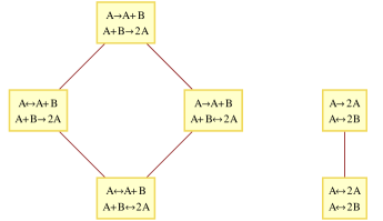
Figure 2: Here we display two of the 35 multistationary bimolecular reversible two-reaction CFSTRs (all inflow and outflow reactions are implied), together with all their respective irreversible multistationary sub-CFSTRs (subnetworks). The poset relation depicted is the subnetwork relation. At left, the reversible CFSTR defined by reactions $A\leftrightarrows A+B\leftrightarrows 2A$ has three multistationary sub-CFSTRs, which are displayed above. Similarly, the example on the right, defined by $2A\leftrightarrows A\leftrightarrows 2B$, has only one multistationary sub-CFSTR. More generally, each of the 35 such reversible networks admits a unique minimal multistationary sub-CFSTR. These minimal subnetworks fall into two classes: 29 of them have the form of the example displayed on the left (the minimal network has two directed reactions), and the remaining 6 have the form of the example on the right (the minimal network has one reversible reaction and one directed reaction). These 35 minimal sub-CFSTRs appear in Figure 3.

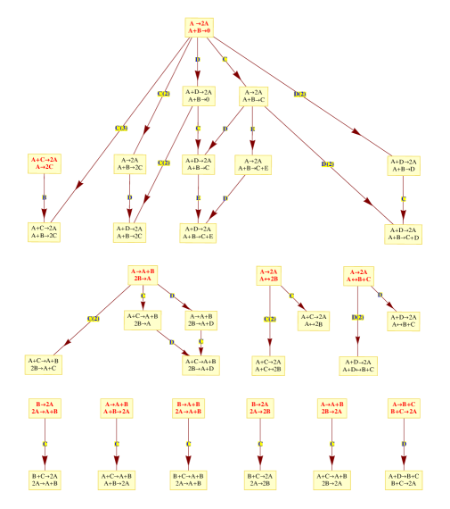
Figure 3: Here we display the 35 multistationary bimolecular two-reaction CFSTRs that are minimal with respect to the subnetwork relation. The poset relation depicted here is that of embedded networks: an arrow points from a network $N$ to a network $G$ if $N$ is an embedded network of $G$. In addition, each such edge is labeled by the species that is removed to obtain $N$ from $G$; for example, $C(2)$ denotes that $G$ contains two molecules of species $C$, and these two are removed from $G$ to obtain $N$. Two networks in the poset are displayed with the same height if they contain the same number of molecules. The 11 CFSTR atoms of multistationarity are marked in bold/red; they are the networks that have only outgoing edges in the figure (at the tops of each component of the poset). All three figures in this work were created in Mathematica.

Finally, we examined the poset obtained from the $N_{i}$ with respect to the relation of ‘embedded networks’ which is displayed in Figure 3. This poset has 11 minimal elements, which are the bimolecular two-reaction CFSTR atoms of multistationarity. It follows that a bimolecular two-reaction (possibly irreversible) CFSTR admits multiple positive steady states if and only if it contains one of these 11 atoms as an embedded network (part 2 of Corollary 7.2).

We end by noting that prohibitively many bimolecular three-reaction networks exist, so currently there is no classification of those CFSTR atoms.

Acknowledgements

This project was initiated by Badal Joshi at a Mathematical Biosciences Institute (MBI) summer workshop under the guidance of Gheorghe Craciun. Badal Joshi was partially supported by a National Science Foundation grant (EF-1038593). Anne Shiu was supported by a National Science Foundation postdoctoral fellowship (DMS-1004380). The authors thank Dan Siegal-Gaskins for sharing AutoIt code which enabled the automated analysis of networks by the CRN Toolbox.

References

- [1] Jonathan Bennett and AutoIt Team, AutoIt v3, Available at http://autoitscript.com/autoit3/index.shtml, 2010.
- [2] Carsten Conradi, Dietrich Flockerzi, Jörg Raisch, and Jörg Stelling, Subnetwork analysis reveals dynamic features of complex (bio)chemical networks, Proc. Natl. Acad. Sci. USA 104 (2007), no. 49, 19175–19180.
- [3] Gheorghe Craciun and Martin Feinberg, Multiple equilibria in complex chemical reaction networks. I. The injectivity property, SIAM J. Appl. Math. 65 (2005), no. 5, 1526–1546.
- [4] , Multiple equilibria in complex chemical reaction networks: extensions to entrapped species models, IEE P. Syst. Biol. 153 (2006), 179–186.
- [5] , Multiple equilibria in complex chemical reaction networks. II. The species-reaction graph, SIAM J. Appl. Math. 66 (2006), no. 4, 1321–1338.
- [6] , Multiple equilibria in complex chemical reaction networks: Semiopen mass action systems, SIAM J. Appl. Math. 70 (2010), no. 6, 1859–1877.
- [7] Gheorghe Craciun, J. William Helton, and Ruth J. Williams, Homotopy methods for counting reaction network equilibria, Math. Biosci. 216 (2008), no. 2, 140–149.
- [8] Anastasia C. Deckard, Frank T. Bergmann, and Herbert M. Sauro, Enumeration and online library of mass-action reaction networks, Available at arXiv/0901.3067, 2009.
- [9] Phillipp Ellison, The advanced deficiency algorithm and its applications to mechanism discrimination, Ph.D. thesis, University of Rochester, 1998.
- [10] Phillipp Ellison, Martin Feinberg, and Haixia Ji, Chemical reaction network toolbox, Available at http://www.che.eng.ohio-state.edu/~feinberg/crnt/, 2011.
- [11] Martin Feinberg, Chemical reaction network structure and the stability of complex isothermal reactors I. The deficiency zero and deficiency one theorems, Chem. Eng. Sci. 42 (1987), no. 10, 2229–2268.
- [12] Martin Feinberg, Chemical reaction network structure and the stability of complex isothermal reactors II. Multiple steady states for networks of deficiency one, Chemical Engineering Science 43 (1988), no. 1, 1–25.
- [13] Elisenda Feliu and Carsten Wiuf, Enzyme sharing as a cause of multistationarity in signaling systems, J. R. Soc. Interface (2011).
- [14] Fritz Horn and Roy Jackson, General mass action kinetics, Arch. Ration. Mech. Anal. 47 (1972), no. 2, 81–116.
- [15] Haixia Ji, Uniqueness of equilibria for complex chemical reaction networks, Ph.D. thesis, Ohio State University, 2011.
- [16] Badal Joshi, Classification of multistationary one-reaction continuous-flow stirred-tank reactors, In preparation, 2012.
- [17] Badal Joshi and Anne Shiu, Simplifying the Jacobian Criterion for precluding multistationarity in chemical reaction networks, SIAM J. Appl. Math. 72 (2012), no. 3, 857–876.
- [18] Igor Klep, Karl Fredrickson, and Bill Helton, Chemical reaction network software (under Mathematica), Available at http://www.math.ucsd.edu/~chemcomp/, 2008.
- [19] Casian Pantea, BioNetX, Available at http://cap.ee.ic.ac.uk/~cpantea/, 2010.
- [20] Casian Pantea and Gheorghe Craciun, Computational methods for analyzing bistability in biochemical reaction networks, Circuits and Systems (ISCAS), Proceedings of 2010 IEEE International Symposium on, IEEE, 2010, pp. 549–552.
- [21] Anne Shiu, The smallest multistationary mass-preserving chemical reaction network, Lect. Notes Comput. Sc. 5147 (2008), 172–184.
- [22] Dan Siegal-Gaskins, Erich Grotewold, and Gregory Smith, The capacity for multistability in small gene regulatory networks, BMC Syst. Biol. 3 (2009), no. 1, 96.
- [23] Dan Siegal-Gaskins, Maria Katherine Mejia-Guerra, Gregory D. Smith, and Erich Grotewold, Emergence of switch-like behavior in a large family of simple biochemical networks, PLoS Comput. Biol. 7 (2011), no. 5, e1002039.
- [24] Thomas Wilhelm, The smallest chemical reaction system with bistability, BMC Syst. Biol. 3 (2009), 90.
- [25] Thomas Wilhelm and Reinhart Heinrich, Smallest chemical reaction system with Hopf bifurcation, J. Math. Chem. 17 (1995), no. 1, 1–14.