Dynamically excited outer Solar System objects in the Hubble Space Telescope archive

Abstract

We present the faintest mid ecliptic latitude survey in the second part of HST archival search for outer Solar System bodies. We report the discovery of 28 new trans-Neptunian objects and 1 small centaur ($R\sim 2$km) in the band $5^{\circ}-20^{\circ}$ off the ecliptic. The inclination distribution of these excited objects is consistent with the distribution derived from brighter ecliptic surveys. We suggest that the size and inclination distribution should be estimated consistently using suitable surveys with calibrated search algorithms and reliable orbital information.

1. Introduction

Trans-Neptunian objects (TNOs) represent the leftovers of the same planetesimals from which the planets in the solar system formed. TNOs offer a unique opportunity for testing theories of the growth and collisional history of planetesimals and the dynamical evolution of the giant planets (Kenyon & Bromley, 2004; Morbidelli et al., 2008). The study of the orbital distribution of TNOs has shown the existence of multiple distinct dynamical populations (Levison & Stern, 2001; Brown, 2001) with different colors (Gulbis et al., 2010; Doressoundiram et al., 2008) and size distributions (Bernstein et al., 2004; Fuentes & Holman, 2008).

The population of small ($\sim$50 km) TNOs contains multiple significant clues to understanding the formation of the Solar System. There are more faint than bright TNOs in the Solar System, which means that faint TNOs are a more thorough dynamical tracer, and that some subtle clues in the dynamical distribution of TNOs may only be revealed by studying this population. Additionally, Pan & Sari showed that the size distribution of objects at this size, and in particular the size at which the size distribution undergoes a change in slope, records the collisional history and intrinsic strength of the TNO population.

Because of the importance of these small — and therefore faint, with R$>$25 and in some cases R$>$27 — TNOs, a great deal of effort has been dedicated to searching for faint TNOs (Chiang & Brown, 1999; Gladman et al., 2001; Allen et al., 2002; Bernstein et al., 2004; Petit et al., 2006; Fraser et al., 2008; Fuentes & Holman, 2008; Fraser & Kavelaars, 2009; Fuentes et al., 2009, 2010). These surveys have been concentrated near the ecliptic, where the sky plane density of objects is largest, since TNOs pass through the ecliptic, regardless of inclination. However, TNOs with inclination $i$ spend most of their time at ecliptic latitudes $\pm i$. Few deep TNO surveys have been carried out at ecliptic latitudes greater than a few degrees. Consequently, elaborate debiasing techniques have been developed (Brown, 2001; Elliot et al., 2005; Gulbis et al., 2010) to derive the true inclination distribution of the TNO population. There have been no direct measurements of the inclination distribution of faint TNOs to date.

The Hubble Space Telescope (HST) presents a unique opportunity in TNO studies by observing across the entire sky. Observations made with HST are deep, with a single 500 second exposure with the Advanced Camera for Surveys (ACS) reaching $\sim$27th magnitude, depending on the bandpass. The combination of these two factors implies that faint TNOs appear serendipitously in a large fraction of all HST images, including fields both on and off the ecliptic. The HST archive, therefore, offers the opportunity to probe the history of the Solar System by measuring the properties of faint TNOs at a wide range of ecliptic latitudes.

We have developed a pipeline that harvests these serendipitous TNOs from archival HST/ACS data (Fuentes et al., 2010, hereafter F10). In F10, we searched ACS data within 5 degrees of the ecliptic and discovered 14 TNOs, including one binary object. Here we expand this search to higher ecliptic latitude, 5–20 degrees. In Section 2 we briefly summarize our field selection criteria and data processing pipeline. Section 3 presents the objects discovered in this mid-latitude search and their orbital parameter distribution. In Section 4 we use this survey to test our current models of inclination distribution.

2. Data

We follow the same criteria described in F10 for quick identification of objects with TNO-like orbits in data taken with ACS/WFC. In this survey we considered fields taken at ecliptic latitudes in the range from 5 to 20 degrees, and for which the total exposure time within a pointing was over 1,500 seconds in at least three images. The Multimission Archive at STScI (MAST) lists data from 1,141 different HST orbits that meet these criteria that were available as of June 4th, 2010 (See Fig. 1).

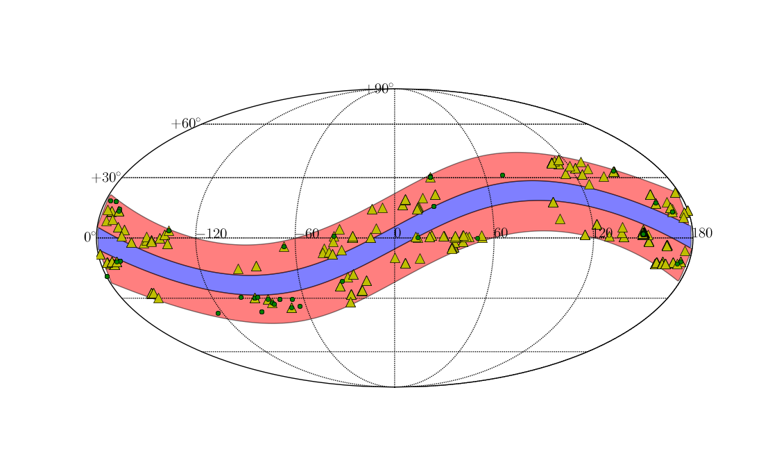
Figure 1.— Map of the sky in J2000 coordinates. The region we chose to select our pointings from is shown in red, that in blue is the region F10 analyzed. The locations of all data considered are plotted as yellow triangles. The green circles are fields that were not surveyed due to problems in the processing or because the sky density yielded too many false positives. Note that there is a concentration of such fields near the galactic center ($-93.6,-29$) where the star density is highest.

2.1. Pipeline

In order to allow the implantation of a control population we considered flat-fielded and undistorted images, as well as the filter dependent PSF models and field distortions explained in Anderson & King (2000).

The pipeline uses the orbital solution and photometric parameters in each image to create and implant the control population. After the images have been cleaned of cosmic rays (CR) using a Laplacian filter the images are ready to be searched for moving objects.

As the motion on the sky of a TNO varies greatly with its orbital elements, we compile a set of elements that produce distinct tracks in the images. For each set of elements in the set we produce sample PSF tracks that are then used to find consistent sources in the images. Finally our algorithm links sources among the images in the set, finding all those that appear in at least 3 of them.

Then, a set of images around all plausible combinations of detections are created to be scouted by a trained operator in order to spot obvious contamination by chance alignment, elongated objects, poorly subtracted CRs, etc.

2.2. Control Population

The detection and identification of a TNO in a given field of view will depend on the characteristics of the observation and the search algorithm. In this project we need to characterize our search method to understand how efficient it is in finding a moving object in the trans-Neptunian region and what variables affect the detection.

We approach this problem by creating a synthetic population that is taken from two different orbital distributions. One is chosen to resemble the semimajor axis distribution of the TNO population so that objects will look like what we expect are typical TNOs. The second distribution tries to sample the whole range of possible bound orbits for objects at a distance between 20 and 200 AU, sampling our ability to detect objects with unusual orbits.

For every original image 200 synthetic objects were inserted. Then the detection process continues with no knowledge of which objects are real and which are not. Only when real objects are identified and a detection efficiency function is constructed is the control population position list unveiled.

3. Analysis

We run our automated search algorithm consistently for all 1141 pointings, of which 98 failed due to too large shifts between the images, poor signal to noise, etc. Of the remaining 1045 pointings  only 986 were visually inspected. A typical field would have less than 500 possible detections, so we did not inspect any field that had more than 1,000 false positives. The 29 real objects discovered and their best fit values for their orbital parameters are listed in Table 1.

We use images like those in 2 to evaluate a $\chi^{2}$ statistic when fitting for the orbital parameters of moving objects. This is used in a Markov Chain Monte Carlo (MCMC) method to estimate the posterior distribution function for the orbital parameters of each found object (See Fig. 4 and Fig. 6). The only constraints we considered on the orbital parameters were a zero velocity along the line of sight and a bound Keplerian orbit.

We usually recovered half of the synthetic objects implanted, yielding a reliable measurement of the brightness efficiency funciton for every field. The coadded efficiency function is shown in Fig. 3. This function is well represented by the formula $\Omega_{eff}=\Omega~{}{\rm erfc}(\frac{R-R_{50}}{2w})~{}{\rm deg^{2}}$ where $\Omega=1.83$, $R_{50}=26.44$ and $w=0.29$.

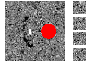
Figure 2.— Coadded image of the Centaur hst39, d= $12.9\pm 0.3$ AU, over a single HST visit showing the apparent motion of the object. The angular size of the Earth at that distance is shown as a red circle. The white bar indicates the relative size of the off ecliptic motion of HST during the visit. The four individual frames are shown in sequence.

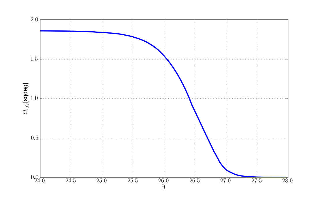
Figure 3.— Total efficiency function for all pointings considered in this survey. It is well represented by the formula $\Omega_{eff}=\Omega~{}{\rm erfc}(\frac{R-R_{50}}{2w})~{}{\rm deg^{2}}$ where $\Omega=1.83$, $R_{50}=26.43$ and $w=0.29$.

Among the moving objects discovered there is an object (hst39) whose orbital parameters confidently constrain it to the Centaur region ($a<30$AU, Trilling et al. in preparation). This object exhibits the least uncertainty on its distance, eccentricity and inclination, as shown in Table 1. This is due to the improved resolution of the motion of HST at the objects’ distance. In 2 we show the four images taken over the course of the pointing coadded.

4. Discussion

Of the orbital parameters for which we obtain the best constrained quantities are the distance to the object and the inclination. The eccentricity is also well constrained for nearer objects.

We present a set of diagrams featuring the inclination (4) and eccentricity (6) as a function of distance for the objects in this survey and for the known object in the outer solar system (5 and 7). The information of known objects was taken from the JPL Horizons website and the distances were computed for January 1st, 2011.

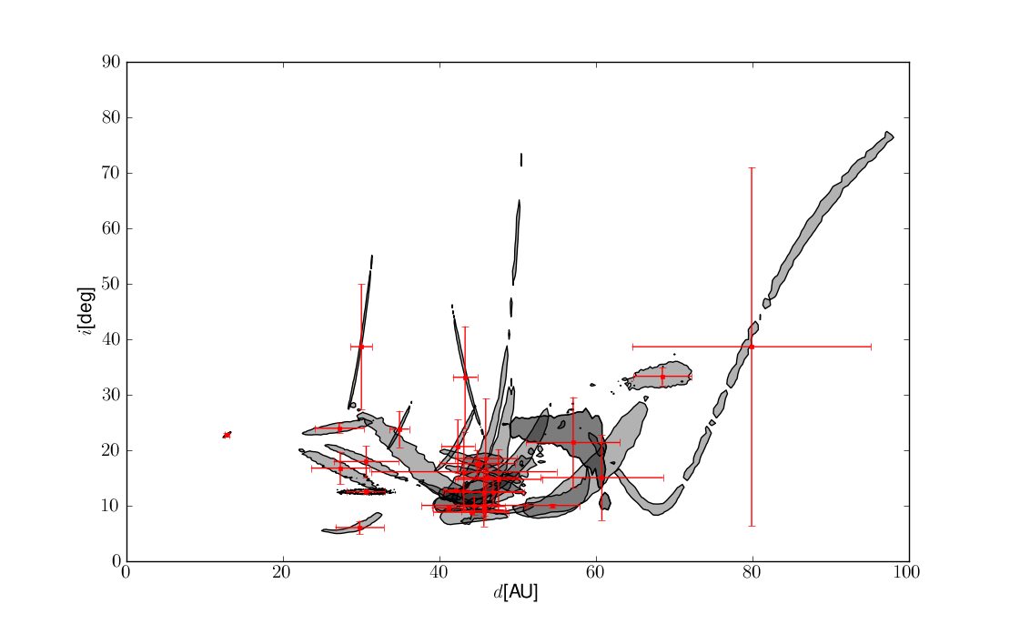
Figure 4.— Distance versus inclination 1$\sigma$ probability contour for each one of the objects in Table 1. The posterior distribution function for each object was estimated with a MCMC as explained in the text. The confidence limits reported in that table are shown in red.

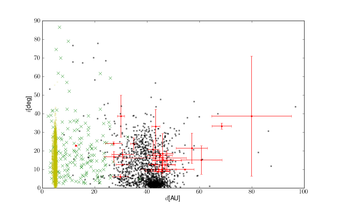
Figure 5.— Distance on Jan 1st, 2011 versus inclination. Outer solar system objects (a$>$30AU, black squares), centaurs (green crosses) and Jupiter trojans (yellow dots) as defined in the JPL lists are shown for comparison. The retrograde solution for hst32 is not shown.

By comparing the shape of the $1-\sigma$ confidence region in distance, inclination and eccentricity in 4 and 6 those quoted in Table 1 we see that nominal gaussian uncertainties are not representative of the actual range of parameters consistent with observations. A worse situation occurs in ground based observations, with the degrading effect from atmospheric seeing on astrometry.

It is interesting to note that all inclination solutions have a lower bound set by the ecliptic latitude of the field where the object was discovered. All but the retrograde solution for hst32 are shown for Fig. 4 and Fig. 5. While most objects have a relatively well constrained distance, data for hst20 is well fit by a wide range of distances and inclinations. In Table 1 its nominal distance is $79.9\pm 15.3$ AU which yields $H=6.9$, the lowest absolute magnitude among our objects. Comparing the probablity distribution for hst20’s orbital parameters in 4 and 6 we see that the lowest inclination corresponds to the highest eccentricity. This solution puts hst20 much closer and in a region with already known objects as can be seen in 5 and 7.

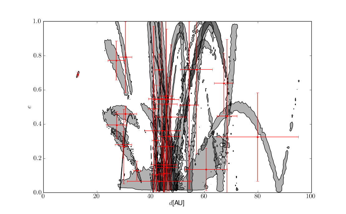
Figure 6.— Distance versus eccentricity 1$\sigma$ probability contour for each one of the objects in Table 1. The confidence limits reported in that table are shown in red.

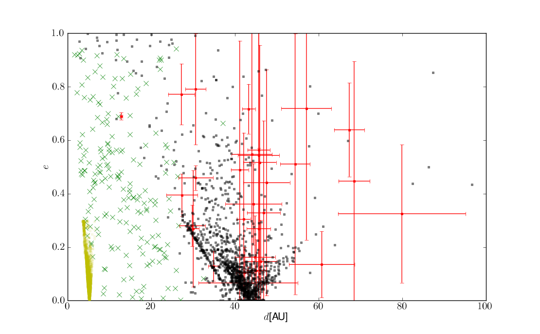
Figure 7.— Distance on Jan 1st, 2011 versus inclination. Outer solar system objects (a$>$30AU, black squares), centaurs (green crosses) and Jupiter trojans (yellow dots) as defined in the JPL lists are shown for comparison.

Some trends can be readily observed, like the high concentration of objects at around $\sim 42$ AU in 4 and 6. The eccentricity is not well contrained except for the few objects closer to the observer. Nevertheless, the data constrains tight relationships between the orbital parameters.

In 7 we see a stream of objects whose eccentricity decreases with distance. These correspond to Plutinos in 3:2 resonance with Neptune. There is compelling evidence for the detection of some Plutinos in our sample by looking at 6 where hst15, hst18, hst25, hst27, and hst31 have distances and eccentricities consistent with being in the 3:2 resonance.

In the inclination vs. distance diagrams we excluded the one retrograde solution allowed by our data (See hst32 in Table 1). That solution is in an area of the parameter space completely void of known objects, while the closer prograde solution (See Table 1) is well accompanied by dynamically hot TNOs.

4.1. Inclination Distribution

Our deep, mid-latitude survey allows us to measure the inclination distribution of small TNOs. We assume there are only two classes of objects in our sample of TNOs, dynamically cold and hot (those with low and high inclinations respectively). We consider a gaussian inclination distribution $f(i)$, and a latitudinal distribution $L(\beta)$ like the ones described in Brown (2001) and Gulbis et al. (2010).

$$f_{j}(i) = \sin(i)~{}\exp(-\frac{i^{2}}{2\sigma_{j}^{2}})~{}~{}~{},$$ (1)

$$p_{j}(i|\beta) = f_{j}(i)\frac{\cos\beta}{\sqrt{\sin^{2}i-\sin^{2}\beta}}~{}~{}~{},$$ (2)

$$L_{j}(\beta) = K_{j}\int_{\beta}^{\pi/2}p_{j}(i|\beta)~{}di~{}~{}~{},$$ (3)

where $j$ represents the hot or cold population and $K_{j}$ is a normalization constant such that $L_{j}(0)=1$. The integrand $p_{j}(i|\beta)$ is the expected inclination distribution from a single observation made at a latitude $\beta$.

We consider a population of objects with distances like those of classical TNOs and inclinations and eccentricities drawn from uniform distributions to compute the total effective survey area. For two or more pointings of the same region of the sky that were observed within a couple of days we calculate the total effective area and detection efficiency depending on the number of objects in our test population that appear in multiple pointings. The result is a set of independent effective observations with different detection efficiencies and observed areas. A total of 777 such observations were identified and visually inspected from the 986 pointings searched.

We then compute the expected number of objects for our survey as a function of inclination considering both the luminosity function and inclination distribution of hot and cold TNOs. We compare this to that of the TNOs discovered in our survey:

$$E(i) = \sum_{k=0}^{N}\sum_{j}\Omega_{k}~{}\eta_{k}~{}L_{j}(\beta_{k})~{}p_{j}(i|\beta_{k})\int_{-\infty}^{\infty}\sigma_{j}(R)dR,$$ (4)

where $\sigma_{j}(R)$ is the number density of hot or cold objects at the ecliptic ($\beta=0$), with the values presented in F10, and $\eta_{k}$ is the detection efficiency function for pointing $k$.

The observed inclination distribution in 8 is the addition of the inclination probability distribution for all 28 TNOs in Table 1. We fit for the width of the hot population inclination distribution $\sigma_{h}$ by comparing the expected and observed probability distributions using the Kolmogorov-Smirnov statistic. The best fit parameter is given by $\sigma_{h}={16.5}_{-3.5}^{+4.5}$ degrees. The effect of considering the cold population is marginal, with less than one cold object expected in our survey whether $\sigma_{c}=2^{\circ}$ or $3^{\circ}$ (as computed in Gulbis et al. (2010) or Brown (2001) for larger TNOs). This result indicates the TNO inclination distribution is independent of size.

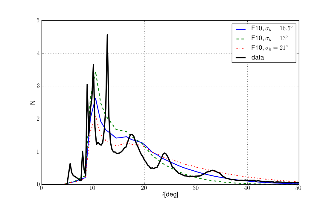
Figure 8.— The inclination probability distribution for all objects found in this survey is shown as a continuous black line. The expected probability distribution for different models consider the luminosity function in F10 and $\sigma_{c}=3^{\circ}$. The best fit for $\sigma_{h}=16.5^{\circ}$ is shown as a blue solid line. The limits for the $1-\sigma$ confidence level are also shown as a dashed green line and a dashed-dotted red line ($\sigma_{h}=13^{\circ},~{}21^{\circ}$ respectively).

There is a caveat in the the expected distribution of objects presented in 8. The expected number of hot objects was 50% larger than those in our survey. To better compare expected with observed inclination distributions we adjusted the density per unit area for hot objects ($\Sigma_{23}$) accordingly, from 0.9 to 0.5. This only affects the number of expected hot objects, and not the shape of the distribution.

5. Conclusions

We have conducted a deep search sensitive to TNOs as faint as R$\sim$27 between ecliptic latitudes $5^{\circ}-20^{\circ}$. These are overwhelmingly dynamically excited objects (only one cold object is expected to appear in our sample), in contrast to surveys performed in the ecliptic where most of the found objects are not dynamically excited. This survey presents a unique opportunity to compare the characteristics of dynamically excited objects to those extrapolated from surveys carried out near the ecliptic.

The inclination distribution of TNOs has been modeled primarily with objects discovered near the ecliptic plane Brown (2001); Gulbis et al. (2010). The double gaussian model introduced by Brown (2001) recognized the existence of two different populations in the classical TNOs, one dynamically excited and the other with seemingly unperturbed near-circular orbits. Further differences in surface properties Doressoundiram et al. (2008) and luminosity function Bernstein et al. (2004); Fuentes et al. (2010); Fraser et al. (2010) have been reported in the literature, hinting on an underlying difference in size distribution and origin.

From our survey we can constrain the width of the hot inclination distribution $\sigma_{h}={16.5}_{-3.5}^{+4.5}$ degrees. Changing this parameter to the 1-$\sigma$ confidence limits gives a significantly poorer representation of the observed distribution. The fact this result is so close to that found by Brown (2001) is an indication that both large and small objects have the same inclination distribution. Comparison to the Deep Ecliptic Survey (DES) inclination distributions in Gulbis et al. (2010) are difficult since we do not have enough orbital information to identify our objects in each of the DES categories.

There are about 500 TNOs discovered in deep, well callibrated surveys. This is enough to fit the luminosity function and inclination distribution in a self consistent manner for the hot, cold, and Plutino populations. The main difficulty for this is the poor constraint on the inclination that is obtained from deep ground based surveys. This can lead to confusion and could explain the discrepancy in the overall number density between those discovered from the ground (that carry most of the statistical weight in the F10 luminosity function) and our survey.

The single centaur found at $d=13$AU in this survey (hst39) has an estimated radius of $2$km if an albedo typical of TNOs p$\sim$7% is assumed (Stansberry et al., 2008). This is one of the smallest object found in the outskirts of the Solar System, close in size to the 500-m sized TNO discovered by occultations (Schlichting et al., 2009). This discovery places a measurement of the Centaur size distribution at a size that is comparable to the known members of the Jupiter family of comets (JFCs, Trilling et al. in preparation).

Table 1Found Objects

${\rm Name}$	${\rm MJD}$	${\rm RA}$	${\rm Dec}$	${\rm Filter}$	$\overline{m}$	$R$	$H$	${\rm opp\_ang}$	$d$	$i$	$e$
								$[deg]$	$[AU]$	$[deg]$
hst15	$53137.86081$	10:02:31.39	$+$02:36:23.94	F814W	$26.9$	$26.2\pm 0.3$	$12.4$	$99.0$	$27.3\pm 3.7$	$16.9\pm 2.9$	$0.4\pm 0.1$
hst16	$53138.79391$	10:02:24.75	$+$02:02:28.69	F814W	$26.1$	$25.4\pm 0.1$	$9.5$	$98.3$	$44.8\pm 4.8$	$17.7\pm 2.4$	$0.2\pm 0.2$
hst17	$53140.59322$	10:00:33.01	$+$02:39:42.18	F814W	$26.6$	$25.9\pm 0.2$	$10.0$	$95.9$	$44.5\pm 6.7$	$10.1\pm 1.6$	$0.4\pm 0.2$
hst18	$53140.65985$	10:00:18.85	$+$02:42:45.20	F814W	$26.5$	$25.8\pm 0.2$	$11.6$	$95.8$	$30.7\pm 4.2$	$18.0\pm 2.8$	$0.5\pm 0.0$
hst19	$53294.08604$	10:02:47.14	$+$02:25:02.01	F814W	$24.6$	$23.9\pm 0.4$	$8.2$	$51.3$	$43.3\pm 1.6$	$33.2\pm 9.2$	$0.7\pm 0.1$
hst20	$53336.93747$	10:02:40.46	$+$02:02:44.59	F814W	$26.0$	$25.3\pm 0.1$	$6.9$	$93.7$	$79.9\pm 15.3$	$38.7\pm 32.3$	$0.3\pm 0.3$
hst21	$53456.68278$	09:57:50.61	$+$02:36:05.01	F814W	$26.9$	$26.2\pm 0.1$	$10.2$	$143.3$	$45.7\pm 4.9$	$12.5\pm 4.3$	$0.5\pm 0.5$
hst22	$53456.68278$	09:58:02.27	$+$02:36:25.01	F814W	$26.8$	$26.1\pm 0.3$	$10.5$	$143.3$	$41.1\pm 2.1$	$9.7\pm 0.4$	$0.5\pm 0.5$
hst23	$53458.48194$	09:59:21.43	$+$01:56:07.15	F814W	$26.2$	$25.5\pm 0.7$	$9.5$	$142.0$	$45.9\pm 3.9$	$18.6\pm 10.8$	$0.5\pm 0.4$
hst24	$53599.42875$	22:17:22.16	$+$00:16:47.33	F814W	$26.3$	$25.6\pm 0.1$	$8.8$	$168.2$	$54.4\pm 3.6$	$10.1\pm 0.3$	$0.5\pm 0.5$
hst25	$53406.30378$	07:17:46.09	$+$37:39:07.57	F606W	$24.3$	$23.7\pm 0.1$	$9.5$	$148.6$	$30.0\pm 1.4$	$38.7\pm 11.3$	$0.3\pm 0.2$
hst26	$53837.23799$	11:19:58.11	$+$12:59:04.06	F555W	$24.7$	$24.1\pm 0.1$	$8.1$	$143.4$	$45.7\pm 2.8$	$9.1\pm 2.8$	$0.3\pm 0.3$
hst27	$53739.17629$	11:20:09.98	$-$12:10:54.78	F814W	$25.8$	$25.1\pm 0.1$	$10.3$	$107.0$	$34.9\pm 1.2$	$23.9\pm 3.3$	$0.1\pm 0.1$
hst28	$53871.90188$	21:40:09.23	$-$23:41:43.81	F606W	$27.3$	$26.6\pm 0.1$	$9.4$	$96.3$	$60.8\pm 7.8$	$15.1\pm 7.7$	$0.1\pm 0.1$
hst29	$52687.02644$	08:09:02.07	$+$06:43:45.38	F814W	$24.8$	$24.1\pm 0.1$	$8.5$	$154.3$	$42.1\pm 1.6$	$12.8\pm 0.1$	$0.3\pm 0.3$
hst30	$52846.01904$	00:26:58.72	$+$18:57:56.91	F814W	$25.3$	$24.6\pm 0.1$	$9.0$	$108.2$	$42.4\pm 2.1$	$20.7\pm 4.8$	$0.1\pm 0.1$
hst31	$53082.65966$	06:33:56.04	$+$17:47:33.54	F555W	$26.3$	$25.6\pm 0.1$	$11.5$	$99.6$	$29.8\pm 3.1$	$6.1\pm 1.2$	$0.3\pm 0.1$
hst32	$53011.80363$	10:57:26.54	$-$03:31:25.46	F814W	$26.1$	$25.5\pm 0.3$	$8.5$	$119.3$	$57.1\pm 6.0$	$21.5\pm 8.2$	$0.7\pm 0.5$
hst32							$7.8$		$67.3\pm 3.6$	$153.6\pm 1.6$	$0.6\pm 0.2$
hst33	$53109.33262$	10:00:57.23	$+$02:31:20.99	F814W	$26.8$	$26.1\pm 0.3$	$10.1$	$126.2$	$45.7\pm 2.7$	$10.0\pm 0.5$	$0.6\pm 0.5$
hst34	$53110.53235$	10:00:42.38	$+$02:34:57.64	F814W	$26.9$	$26.2\pm 0.1$	$10.3$	$125.0$	$44.1\pm 4.8$	$8.9\pm 0.1$	$0.5\pm 0.5$
hst35	$52936.79893$	09:59:43.32	$+$01:53:12.54	F814W	$26.4$	$25.8\pm 0.1$	$8.0$	$59.7$	$68.5\pm 3.7$	$33.4\pm 1.6$	$0.4\pm 0.4$
hst36	$53127.86201$	10:00:13.57	$+$02:39:33.91	F814W	$27.1$	$26.4\pm 0.4$	$12.1$	$108.0$	$30.6\pm 2.5$	$12.6\pm 0.4$	$0.8\pm 0.2$
hst37	$53133.79487$	10:00:03.34	$+$02:37:19.99	F814W	$27.5$	$26.8\pm 0.2$	$13.0$	$102.3$	$27.2\pm 3.2$	$24.0\pm 0.9$	$0.8\pm 0.1$
hst38	$53134.32813$	09:59:52.54	$+$02:25:36.08	F814W	$26.4$	$25.7\pm 0.1$	$9.7$	$101.8$	$46.2\pm 3.9$	$15.1\pm 1.8$	$0.1\pm 0.2$
hst39	$53129.06194$	10:00:02.50	$+$02:23:52.38	F814W	$26.7$	$26.0\pm 0.1$	$15.5$	$106.9$	$12.9\pm 0.3$	$22.8\pm 0.4$	$0.7\pm 0.0$
hst40	$53129.06194$	09:59:54.66	$+$02:24:28.75	F814W	$26.2$	$25.6\pm 0.1$	$9.6$	$106.9$	$45.1\pm 2.3$	$17.7\pm 1.0$	$0.1\pm 0.1$
hst41	$53111.53199$	09:58:56.65	$+$02:14:44.58	F814W	$26.8$	$26.1\pm 0.2$	$9.9$	$123.7$	$47.6\pm 5.6$	$14.8\pm 5.4$	$0.4\pm 0.4$
hst42	$53102.66744$	09:59:27.71	$+$01:57:12.46	F814W	$26.6$	$25.9\pm 0.1$	$9.8$	$132.6$	$46.9\pm 4.0$	$12.6\pm 2.3$	$0.3\pm 0.3$
hst43	$52845.31524$	14:13:16.34	$-$01:42:04.90	F435W	$26.5$	$25.5\pm 0.1$	$9.7$	$89.8$	$43.1\pm 11.8$	$16.2\pm 7.2$	$0.1\pm 0.1$

Note. — All objects found in this work are shown with their photometric and astrometric properties. Positions given for the first detections. The barycentric distance $d$ and inclination $i$ were estimated from a MCMC with a parameterization given by the Orbfit code (Bernstein & Khushalani, 2000). Though some objects were discovered in the same field, the epoch of the observations is different. The Solar System magnitude $H=V+5\log{d~{}\Delta}$, a function of the $V$ magnitude $d$ and the distance to the observer $\Delta$, is computed assuming the phase angle is small and that the V-R color for all objects is 0.6. The conversion between HST filters and the Johnson system are detailed in F10.

References

- Allen et al. (2002) Allen, R. L., Bernstein, G. M., & Malhotra, R. 2002, AJ, 124, 2949
- Anderson & King (2000) Anderson, J., & King, I. R. 2000, PASP, 112, 1360
- Bernstein & Khushalani (2000) Bernstein, G., & Khushalani, B. 2000, AJ, 120, 3323
- Bernstein et al. (2004) Bernstein, G. M., Trilling, D. E., Allen, R. L., Brown, M. E., Holman, M., & Malhotra, R. 2004, AJ, 128, 1364
- Brown (2001) Brown, M. E. 2001, AJ, 121, 2804
- Chiang & Brown (1999) Chiang, E. I., & Brown, M. E. 1999, AJ, 118, 1411
- Doressoundiram et al. (2008) Doressoundiram, A., Boehnhardt, H., Tegler, S. C., & Trujillo, C. 2008, Color Properties and Trends of the Transneptunian Objects, ed. M. A. Barucci, H. Boehnhardt, D. P. Cruiksank, & A. Morbidelli, 91–104
- Elliot et al. (2005) Elliot, J. L., et al. 2005, AJ, 129, 1117
- Fraser et al. (2010) Fraser, W. C., Brown, M. E., & Schwamb, M. E. 2010, Icarus, 210, 944
- Fraser & Kavelaars (2009) Fraser, W. C., & Kavelaars, J. J. 2009, AJ, 137, 72
- Fraser et al. (2008) Fraser, W. C., et al. 2008, Icarus, 195, 827
- Fuentes et al. (2009) Fuentes, C. I., George, M. R., & Holman, M. J. 2009, ApJ, 696, 91
- Fuentes & Holman (2008) Fuentes, C. I., & Holman, M. J. 2008, AJ, 136, 83
- Fuentes et al. (2010) Fuentes, C. I., Holman, M. J., Trilling, D. E., & Protopapas, P. 2010, in preparation
- Gladman et al. (2001) Gladman, B., Kavelaars, J. J., Petit, J.-M., Morbidelli, A., Holman, M. J., & Loredo, T. 2001, AJ, 122, 1051
- Gulbis et al. (2010) Gulbis, A. A. S., Elliot, J. L., Adams, E. R., Benecchi, S. D., Buie, M. W., Trilling, D. E., & Wasserman, L. H. 2010, AJ, 140, 350
- Kenyon & Bromley (2004) Kenyon, S. J., & Bromley, B. C. 2004, AJ, 128, 1916
- Levison & Stern (2001) Levison, H. F., & Stern, S. A. 2001, AJ, 121, 1730
- Morbidelli et al. (2008) Morbidelli, A., Levison, H. F., & Gomes, R. 2008, The Dynamical Structure of the Kuiper Belt and Its Primordial Origin, ed. Barucci, M. A., Boehnhardt, H., Cruikshank, D. P., & Morbidelli, A., 275–292
- Petit et al. (2006) Petit, J.-M., Holman, M. J., Gladman, B. J., Kavelaars, J. J., Scholl, H., & Loredo, T. J. 2006, MNRAS, 365, 429
- Schlichting et al. (2009) Schlichting, H. E., Ofek, E. O., Wenz, M., Sari, R., Gal-Yam, A., Livio, M., Nelan, E., & Zucker, S. 2009, Nature, 462, 895
- Stansberry et al. (2008) Stansberry, J., Grundy, W., Brown, M., Cruikshank, D., Spencer, J., Trilling, D., & Margot, J.-L. 2008, Physical Properties of Kuiper Belt and Centaur Objects: Constraints from the Spitzer Space Telescope, ed. Barucci, M. A., Boehnhardt, H., Cruikshank, D. P., & Morbidelli, A. (The Solar System Beyond Neptune), 161–179