Chemical Abundances of Red Giant Stars in the Globular Cluster M107 (NGC 6171)

Abstract

We present chemical abundances of Al and several Fe–Peak and neutron–capture elements for 13 red giant branch stars in the Galactic globular cluster NGC 6171 (M107). The abundances were determined using equivalent width and spectrum synthesis analyses of moderate resolution (R $\sim$15,000), moderate signal–to–noise ratio ($\langle$S/N$\rangle$$\sim$80) spectra obtained with the WIYN telescope and Hydra multifiber spectrograph. A comparison between photometric and spectroscopic effective temperature estimates seems to indicate a reddening value of E(B–V)=0.46 may be more appropriate for this cluster than the more commonly used value of E(B–V)=0.33. Similarly, we found that a distance modulus of (m–M)_V$\approx$13.7 provided reasonable surface gravity estimates for the stars in our sample. Our spectroscopic analysis finds M107 to be moderately metal–poor with $\langle$[Fe/H]$\rangle$=–0.93 and also exhibits a small star–to–star metallicity dispersion ($\sigma$=0.04). These results are consistent with previous photometric and spectroscopic studies. Aluminum appears to be moderately enhanced in all program stars ($\langle$[Al/Fe]$\rangle$=+0.39, $\sigma$=0.11). The relatively small star–to–star scatter in [Al/Fe] differs from the trend found in more metal–poor globular clusters, and is more similar to what is found in clusters with [Fe/H]$\gtrsim$–1. The cluster also appears to be moderately r– process enriched with $\langle$[Eu/La]$\rangle$=+0.32 ($\sigma$ = 0.17).

1 INTRODUCTION

The old paradigm that globular clusters represent single, coeval stellar populations has been overturned by the discovery of multiple, discrete populations existing in seemingly “normal” clusters (e.g., see Renzini 2008; Piotto 2009; Milone et al. 2010 for recent reviews). While it has long been known that essentially all globular clusters exhibit significant star–to–star abundance variations for the elements carbon to aluminum (e.g., see Gratton et al. 2004 and references therein), the connection between the light element variations and existence of multiple populations is only now becoming more clear. It is now thought that most clusters contain (at least) two separate generations of stars. These populations exhibit identical [Fe/H] ratios, but differ in their light element abundances (e.g., Carretta et al. 2009a). The first generation or “primordial” stars reflect the light element abundance patterns produced by type II supernovae (SNe), which are nearly identical to the metal–poor halo composition. The second generation stars appear to have formed from gas that experienced varying degrees of high–temperature proton–capture nucleosynthesis, and are therefore in general O/Mg–poor and Na/Al–rich compared to the typical halo field star. Interestingly, the second generation tends to be the dominant population in most clusters, and the number of first generation stars retained is likely a function of cluster mass (Carretta et al. 2009a). While the more massive clusters tend to exhibit the most extreme light element abundance and multiple population characteristics, smaller clusters like M107, which do not appear to contain a significant fraction of extremely O/Mg–poor and Na/Al–rich stars, may be useful probes for determining the processes which produce the second generation in globular clusters.

The Galactic globular cluster M107 is of relatively average mass ($\sim$10⁵ M_☉; Piatek et al. 1994), but is a factor of two more metal–rich than the average globular cluster (Harris 1996; updated 2010). A compilation of multiple photometric and moderate resolution spectroscopic analyses (Pilachowski et al. 1981; Smith & Perkins 1982; Smith & Manduca 1983; Zinn & West 1984; Carretta & Gratton 1997; Ferraro et al. 1999; Carretta et al. 2009a, 2009b) yields a metallicity value between [Fe/H]=–0.83 and –1.07. However, most of the spectroscopic measurements are based on small sample sizes ($\lesssim$ 5 stars). Although globular clusters tend to exhibit a wide range in horizontal branch (HB) morphologies at a given metallicity, the HB of M107 is dominated by red HB and RR Lyrae stars (Sandage & Katem 1964; Dickens & Rolland 1972; Sandage & Roques 1982; Da Costa et al. 1984; Ferraro et al. 1991; Cudworth et al. 1992) which is clearly reflected in the (B–R)/(B+V+R) HB ratio estimate by Lee et al. (1994) of –0.76$\pm$0.08. M107 lacks a significant population of blue HB and blue hook stars that are typically found in some of the more massive clusters exhibiting the largest light element abundance variations and may suggest that this cluster did not experience strong helium enrichment.

While the [Fe/H], [O/Fe], and [Na/Fe] ratios have been determined for $\sim$30 red giant branch (RGB) stars in M107, chemical abundances for Al and heavier $\alpha$ elements are only available for $\sim$5 stars, and the neutron–capture element abundances have never been explored. Therefore, we present for the first time moderate resolution spectroscopic abundances of Al, Ti, Sc, Ni, Fe, La, and Eu for 13 RGB stars in this cluster. In section 2 we describe the selection of stars for observation and data reduction. Section 3 contains the radial velocity measurements and cluster membership evaluations for individual stars. Section 4 describes the procedures for estimating model atmosphere parameters and measuring the chemical abundances. Lastly, in section 5 we outline and discuss the results and provide a summary in section 6.

2 OBSERVATIONS AND REDUCTIONS

The observations for all cluster giants were taken at Kitt Peak National Observatory on May 14, 2000 using the WIYN 3.5m telescope instrumented with the Hydra multi–fiber positioner and bench spectrograph. All spectra were obtained with a single Hydra configuration that employed the 2$\arcsec$ red fibers, 316 line mm^-1 echelle grating and red camera, achieving a resolving power of R($\lambda$/$\Delta$$\lambda$)$\approx$15,000. The spectrograph setup was centered near 6660 Å, and the full wavelength coverage spanned from $\sim$6460–6860 Å. Target stars were selected based on photometry from Sandage & Katem (1964), with colors suggesting their location on or near the RGB. The coordinates used in generating the Hydra configuration were taken from the USNO Image and Catalogue Archive. The final sample includes 13 RGB stars spanning a V magnitude range of 13.23–14.66, which corresponds to a luminosity range from the RGB tip down to approximately 1 magnitude above the level of the HB (V_HB $\approx$15.7; Buonnano et al. 1989; Ferraro et al. 1991; see also Figure 1).

Basic data reductions were carried out using the standard IRAF routines. Specifically, ccdproc was used to apply the bias level correction and trim the overscan region. The IRAF task dohydra was employed for aperture tracing, scattered light and cosmic ray removal, extraction of the one–dimensional spectra, flat–fielding, wavelength calibration (based on a ThAr comparison source), and sky subtraction. The extracted spectra were then co–added to increase the S/N of the final spectra and continuum fit using a low order spline function. The S/N of the combined spectra ranged from $\sim$60–110.

3 RADIAL VELOCITY MEASUREMENTS AND CLUSTER MEMBERSHIP

Cluster membership was confirmed by comparing radial velocity measurements to the mean value of –34.23 km s^-1 found by Pryor & Meylan (1993). All radial velocities for this study were determined via the IRAF task fxcor, and corrected for the Earth’s motion using rvcorrect. A proper motion study by Cudworth et al. (1992) presents membership probabilities for all stars selected for analysis, with the exception of star 201. Table 1 provides radial velocity measurements and associated uncertainties for each program star, as well as Cudworth’s membership probabilities. The average radial velocity of –31.8 km s^-1 and small velocity dispersion ($\sigma$=2.4 km s^-1 found here are in agreement with previous studies (e.g., Pryor & Meylan 1993; Piatek et al. 1994)

Note that Smith & Hesser (1986) exclude star F as a cluster member based on DDO photometry and identified it as a possible foreground dwarf. However, Cudworth et al. (1992) assigned the star a high membership probability (98$\%$), and we find star F to have a radial velocity that is reasonably consistent with the cluster average at –37.1 km s^-1. Although the radial velocity of star F is $\sim$2$\sigma$ outside the cluster mean, it has an effective temperature, surface gravity, and metallicity that are all consistent with the star being a bona fide member. Therefore, we have included it in our analysis.

4 ANALYSIS

We have analyzed a small sample of RGB stars in M107 for elemental abundances of Al, neutron–capture, and Fe–peak elements in the range of Al to Eu II. IRAF’s splot package was used to measure equivalent widths (EWs) with a single-line EW analyses for unblended lines, and a blended–line function for heavily blended lines or lines subject to hyperfine splitting. The wavelength range of observed spectra is from $\sim$6460-6860 Å. Effective temperatures and surface gravities for individual stars were initially estimated using the cluster’s distance modulus and (V–K)₀ color indices obtained from photometric data. Although Sandage & Katem (1964) provide photometry for all target stars, photometry for initial T_eff estimates was taken from the more recent proper motion study by Cudworth et al. (1992). Star 201 was not included in this study, but Dickens & Rolland (1972) provide colors for 201 transformed from Sandage & Katem (1964). An iterative LTE stellar line analysis program was used to further modify T_eff and microturbulence (v_t) via spectroscopic analyses. Table 2 shows the results of an assessment with respect to abundance sensitivity and associated uncertainties in adopted model atmosphere parameters for all elements considered in this study.

4.1 Model Stellar Atmospheres

Initial T_eff estimates for individual stars were determined through use of the empirical V–K_S color–temperature relation described by Alonso et al. (1999, and erratum from 2001). The V–band photometry was obtained from Cudworth et al. (1992) and Dickens & Rolland (1972), and the K_S–band data were taken from the Two Micron All Sky Survey (2MASS) database (Skrutskie et al. 2006). A color excess value of E(B–V)=0.33 (Webbink 1985; Harris 1996), which is in agreement with the Cudworth et al. (1992) estimate, was initially adopted in order to correct for interstellar reddening and extinction. However, we found that applying this reddening correction produced T_eff values that were at least 150–200K lower than the T_eff estimates derived spectroscopically by imposing excitation equilibrium (see Figure 2). Further investigation of this problem revealed that the color excess for NGC 6171 is not particularly well constrained, with literature values ranging from E(B–V)$\approx$0.25–0.50 (e.g., Smith & Hesser 1986; Salaris & Weiss 1997). Dutra & Bica (2000) noticed a similar inconsistency between their derived value of E(B–V)=0.45, based on 100$\micron$ dust emission, and previously published estimates.

While our data do not permit an explicit measure of interstellar reddening along the clusters line–of–sight, we do find that a near 1:1 correlation between photometric and and spectroscopic T_eff estimates for cluster giants can be achieved if one assumes a reddening near the upper limit of E(B–V)$\approx$0.46 (see Figure 2). Since this larger E(B–V) value is also found in the Schlegel et al. (1998) dust maps, which were accessed via the NED Coordinate Transformation & Galactic Extinction Calculator, we used an average value of E(B–V)=0.46 in the final T_eff calculations. Furthermore, use of the online extinction calculator permitted a rough examination into the prospect of differential reddening across our observed field, which could be an issue given the cluster’s low Galactic latitude (b=23$\arcdeg$). Fortunately, the star–to–star reddening variation did not exceed 0.02 mag, and therefore no additional corrections were applied.

Surface gravities were calculated using the standard relation,

$$log(g)=0.40(M_{bol.}-M_{bol.\sun}+log(g_{\sun})+4(log(T/T_{\sun}))+log(M/M_{\sun}),$$ (1)

and assumed a stellar mass of of 0.8 M_☉. Stellar atmospheres were modeled without convective overshoot by interpolating in the ATLAS9 grid (Castelli et al. 1997). The absolute bolometric magnitudes (M_bol.) were determined by applying the V–band bolometric corrections from Alonso et al. (1999; their equations 17 and 18) to the absolute V–band magnitudes estimated from the distance modulus (m–M)_V=13.76 (Shetrone et al. 2009). In a similar fashion to the reddening estimate, a wide range of distance modulus estimates for this cluster appear in the literature and span from (m–M)_V=15.06 (e.g., Harris 1996) to (m–M)_V=13.76 (Shetrone et al. 2009). However, we chose the smallest available distance modulus because the larger distance moduli yielded surface gravity values that appeared too low for each star’s metallicity and position on the color–magnitude diagram.

Initial model atmospheres were calculated with a metallicity of [Fe/H]$\approx$–1, which is consistent with previous estimates (e.g., Smith & Manduca 1983; Pilachowski 1984; Zinn & West 1984; Ferraro et al. 1991; Carretta et al. 2009a, 2009b), and also assumed a microturbulence value of 2 km s^-1 for all stars. These values were further refined through an iterative process that primarily focused on finalizing the microturbulence value by removing trends in Fe I abundance as a function of reduced width [log(EW/$\lambda$)]. A summary of our final model atmosphere parameters and photometric indicies is provided in Table 3.

4.2 Equivalent Width Analyses, Hyperfine Structure, and Spectrum Synthesis

All element abundances, with the exception of Al, were derived by equivalent width (EW) measurements using IRAF’s splot package. Suitable lines were chosen both by visual inspection and comparison to the Hinkle et al. (2000) Arcturus atlas, which combines a side–by–side profile of the solar and Arcturus spectra. Given the moderate resolution of our spectra, we chose lines for analysis that were not expected to be severely blended. While the abundances of Ti, Fe, Ni, and La were determined by employing the abfind driver in the 2002 version of the LTE line analysis code MOOG (Sneden 1973), the abundances of Al, Sc, and Eu were either determined via the synth spectrum synthesis driver (Al) or the blended line blends driver (Sc and Eu).

For Al, we chose to derive the abundances using full spectrum synthesis of the 6690-6700 Å window because both the 6696 and 6698 Å Al lines are moderately blended with nearby metal and CN lines. For Sc, La, and Eu, the abundance derivation requires taking into account hyperfine structure and/or isotopic broadening. While both Sc and La have only one long–lived, stable isotope (⁴⁵Sc and ¹³⁹La), Eu has two (¹⁵¹Eu and ¹⁵³Eu) that are present in nearly equal proportions. Therefore, our input linelists for Sc and Eu made use of the the hyperfine/isotope data from Prochaska & McWilliam (2000) and Lawler et al. (2001), respectively. Although no hyperfine linelist exists for the 6774 Å La II line used here, we applied the empirical correction given in Johnson & Pilachowski (2010; equation A1) to our measured EWs. The final EWs and abundance ratios, cited as relative to Fe I, are provided in Tables 4 and 5, respectively.

5 RESULTS AND DISCUSSION

5.1 Al Abundances

Large star–to–star light element abundance variations are a ubiquitous feature of globular clusters (e.g., see reviews by Kraft 1994; Gratton et al. 2004). While it is understood that these abundance patterns, in particular those involving the elements between carbon and aluminum, are the result of proton–capture nuclear reactions, the exact production site(s) is (are) not well established. Evolved red giants have deep convective envelopes that can mix proton–capture cycled material from a star’s interior to its photosphere, and this mechanism is clearly responsible for the first dredge–up phenomenon (e.g., Iben 1965). However, observations of similar abundance variations involving heavier elements, from O to Al, in globular cluster stars near the main–sequence and turn off (e.g., Cannon et al. 1998; Gratton et al. 2001; Cohen et al. 2002; Briley et al. 2004a, 2004b; Boesgaard et al. 2005) suggest pollution must play a key role as well. The most commonly suggested pollution sites tend to be either rapidly rotating, massive stars (e.g., Maeder & Meynet 2006) or $\sim$5–8 M_☉ AGB stars (e.g., Ventura & D’Antona 2009). While the AGB scenario tends to be the most commonly accepted, it is likely that both massive and intermediate mass stars play key roles in determining the light element composition of globular cluster stars (see also Renzini 2008 for a recent review). Since Al is the heaviest element that generally exhibits a large abundance range in globular clusters, it requires the highest temperatures to be produced ($\gtrsim$5$\times$10⁷ K) in significant quantities. These temperatures are not expected to be reached at the bottom of the convective envelope in low mass stars with [Fe/H]$\approx$-1, and therefore Al can be used as a tracer for the amount of pollution experienced by M107 stars.

We find the individual [Al/Fe] ratios to be enhanced by an average of $+$0.39 dex with a relatively small dispersion of $\sigma$=0.11 dex. While the full range of [Al/Fe] spans from $+$0.24 to +0.63 dex, only two stars (J and 205) have [Al/Fe]$>$+0.5. The enhancement of Al in star 205 is shown in Figure 3 where we overplot stars N and 205, which have similar T_eff, log(g), and [Fe/H], but differ in their [Al/Fe] ratios by $\sim$0.3 dex.

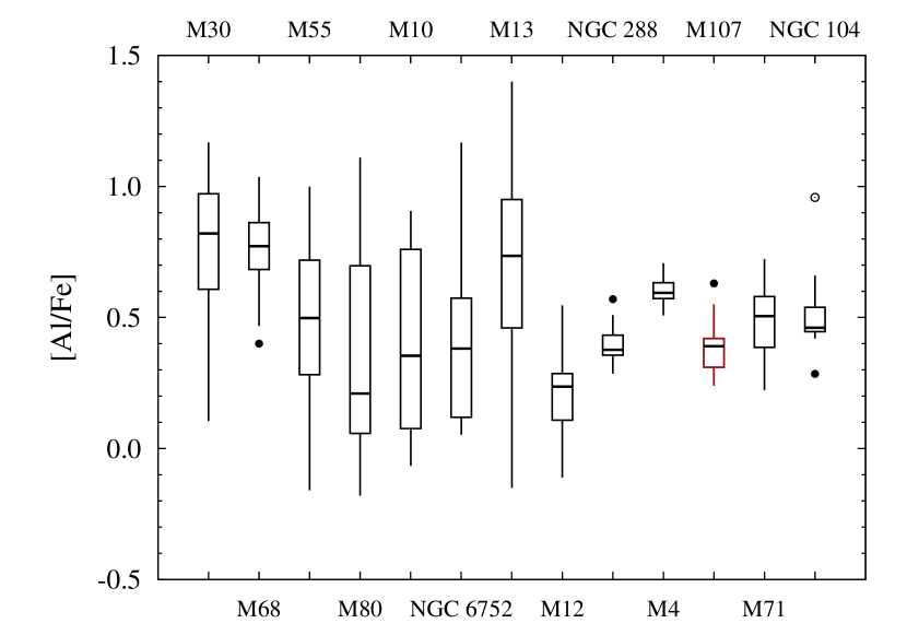
Figure 4: Box plot illustrating [Al/Fe] distribution in 13 galactic globular clusters –2.35 $\lesssim$ [Fe/H] $\lesssim$ –0.75. Clusters are plotted by increasing metallicity. The middle line of each box indicates the median abundance value, and the upper and lower box boundaries represent the third and first quartiles (75^th and 25^th percentile) of the data, respectively. The vertical lines represent the full range of abundance values. Suspected outliers (stars with abundances 1.5 times above the 3^rd, or below the 1^st interquartile range) are designated by filled circles, and outliers (abundances 3.0 times above the 3^rd, or below the 1^st interquartile range) are open circles. M80 from Cavallo et al. (2004); M13 from Johnson et al. (2005); M30, M68, M55, M10, NGC 6752, M12, NGC 288, M4, M71 and NGC 104 from Carretta et al. (2009b); M107 from the current study.

In Figure 4 we show a box plot of the [Al/Fe] ratios for 13 globular clusters ranging in [Fe/H] from approximately –2.35 to –0.80. While it is clear from Figure 4 that the overwhelming majority of globular cluster stars have [Al/Fe]$>$0, there appears to be a significant change in the [Al/Fe] abundance spreads for the more metal–rich clusters, including M107. The metal–poor, and generally more massive, clusters tend to exhibit a full range of [Al/Fe] abundances spanning nearly a factor of 10, but the clusters with [Fe/H]$\gtrsim$–1.2 tend to exhibit abundance spreads of only 0.1–0.5 dex. This observation is not entirely surprising, especially when considered in the context of the commonly assumed paradigm that the light element abundance dispersions in globular clusters are driven primarily by pollution from intermediate mass AGB stars because theoretical Type II SNe and AGB yields tend to converge at [Fe/H]$\gtrsim$–1.2 (e.g., see Figure 22 in Johnson & Pilachowksi 2010 and references therein). This means a cluster like M107, forming from gas polluted by Type II SNe and AGB stars with metallicities near [Fe/H]$\sim$–1, should not exhibit the same large [Al/Fe] spread seen in stars forming from gas polluted by more metal–poor progenitors. Therefore, the observed small [Al/Fe] variations observed in M107 are consistent with its metallicity. However, the average [Al/Fe]=$+$0.39 is at least 0.3 dex lower than the predicted yields of the $\sim$5–6.5 M_☉ AGB stars that are commonly assumed to be the primary polluters in globular clusters (e.g., Ventura & D’Antona 2009; but see also Karakas 2010). The moderate Al enhancement in M107 suggests that the gas from which these stars formed did not exceed an AGB/Type II SN pollution ratio of roughly 20$\%$/80$\%$, respectively. This result is compatible with the observed modest extension of M107’s O–Na anticorrelation seen in Carretta et al. (2009a).

5.2 $\alpha$, Fe–Peak, and Neutron–Capture Elements

Although Ti is often enhanced in globular clusters like the lighter, true $\alpha$ elements (e.g., Mg and Ca), its exact nucleosynthetic origin is unclear. However, M107 does not appear to be an exception as both the [Ti I/Fe] and [Ti II/Fe] ratios indicate that cluster stars are enhanced by an average [Ti/Fe]=$+$0.40 with a relatively small star–to–star dispersion ($\sigma$=0.10). Similarly, the Fe–peak elements, traced here by Sc and Ni, are typically not enhanced in globular cluster stars and tend to exhibit small star–to–star dispersions. We find that M107 fits this trend as Ni exhibits no enhancements on average with $\langle$[Ni/Fe]$\rangle$=0.00 ($\sigma$=0.09) and Sc also appears only moderately enhanced at $\langle$[Sc/Fe]$\rangle$=+0.13 with a small star–to–star dispersion ($\sigma$=0.09). The enhancement of [Ti/Fe] and solar–scaled abundance ratios of [Sc/Fe] and [Ni/Fe] are clearly illustrated in Figure 5, where we show a box plot of all elements measured in this study.

Most stable isotopes of elements heavier than the Fe–peak are produced through either the rapid (r) or slow (s) neutron–capture process (e.g., see review by Sneden et al. 2008). In general, the heavier elements synthesized via the main component of the s–process (e.g., Ba and La) are believed to be primarily produced in lower mass ($\sim$1–3 M_☉) thermally pulsing AGB stars over timescales $\gtrsim$5$\times$10⁸ yrs. In contrast, the exact origin of the r–process is unknown, but it is believed to be associated with core collapse SNe and therefore enrichment should occur on a rapid timescale of $\lesssim$5$\times$10⁷ yrs (e.g., see review by Truran et al. 2002). R–process production is often traced through the element Eu, which is produced almost exclusively by the r-process.

While the star–to–star dispersion for neutron–capture elements in globular clusters is typically larger than that observed for the $\alpha$ and Fe–peak elements (e.g., see Roederer 2011 and references therein), it is almost always smaller than the variations observed for the lighter elements C through Al. However, on average most globular clusters have [Eu/La]$\gtrsim$$+$0.2 (e.g., Gratton et al. 2004), which suggests that the clusters formed rapidly and before a significant amount of s–process enrichment could occur. M107 exhibits this same trend with $\langle$[La/Fe]$\rangle$=$+$0.41 ($\sigma$=0.12), $\langle$[Eu/Fe]$\rangle$=$+$0.73 ($\sigma$=0.13), and $\langle$[Eu/La]$\rangle$=$+$0.32 ($\sigma$=0.17). Although the [Eu/Fe] ratio exhibits the largest abundance range out of all the elements included in this study, the [Eu/Fe] interquartile range is not appreciably different than the other elements. This suggests that the cluster formed from gas that was well mixed and exhibited a nearly homogeneous composition. Lastly, the negligible s–process signature indicates that low and intermediate mass AGB stars did not contribute strongly to the cluster’s primordial composition, which further supports the observed relatively small light element abundance variations observed here and in previous studies.

6 SUMMARY

We present for the first time moderate resolution spectroscopic abundances of Fe, Al, Ti, Sc, Ni, La, and Eu for 13 RGB stars in the globular cluster NGC 6171 (M107). All data for this study were obtained at Kitt Peak National Observatory with the WIYN 3.5m telescope and Hydra multifiber spectrograph using a moderate resolution (R$\sim$15,000) echelle grating. The coadded spectra have a $\langle$S/N$\rangle$ $\sim$80 and cover a wavelength range from $\sim$6460-6860 Å. Program stars range in luminosity from the RGB tip to $\sim$1 magnitude above the level of the HB.

Effective temperatures and surface gravities for individual stars were estimated using the cluster’s distance modulus and (V–K)₀ color indices obtained from photometric data. An iterative LTE stellar line analysis code was employed to further modify T_eff and microturbulence (v_t) via spectroscopic analyses. With the exception of Al, abundances were determined by equivalent width (EW) analyses. For Al we chose to derive abundances using spectrum synthesis to eliminate possible contamination from nearby CN and metal lines. Input linelists were used for Sc and Eu to provide hyperfine structure and/or isotope broadening corrections. An empirical correction was applied to our La II EW measurements as no hyperfine linelist exists for this line.

Given the low galactic latitude of this cluster and close relative proximity to the galactic center (b=23$\arcdeg$ and R_GC=3.3 kpc, respectively), interstellar reddening and extinction can be a possible concern. Reddening values and distance moduli found in literature were not very well constrained, but by assuming a color excess value close to the upper limit found in literature, E(B–V) $\sim$0.46, we find a near 1:1 correlation between photometric and spectroscopic T_eff estimates. Similarly, we chose the smallest available distance modulus, (m–M)_V=13.76, because the larger distance moduli yielded surface gravity values that appeared too low for each star’s metallicity and position on the color magnitude diagram.

We confirm that M107 is moderately metal–rich, with average [Fe/H]=–0.93 ($\sigma$=0.04), which is consistent with previous photometric and spectroscopic studies. Program stars indicate a small star–to–star metallicity spread of 0.12 dex suggesting M107 is a bona fide monometallic cluster. Carretta et al. (2009a) finds a similar star–to–star spread in [Fe/H], 0.18 dex, and the same $\sigma$ value, 0.04, for 33 stars in this cluster. The HB of M107 is dominated by red HB stars ((B–R)/(B+V+R)=–0.76$\pm$0.08) and RR Lyrae variables, which would not be unexpected for its metallicity, and lacks a significant population of blue HB and blue hook stars. This may indicate that M107 did not experience strong helium enrichment typically demonstrated by some of the more massive clusters that also tend to exhibit the largest light element abundance variations.

We find that the [Al/Fe] ratio is enhanced in all cluster stars at $\langle$[Al/Fe]$\rangle$=$+$0.39 ($\sigma$=0.11) with only two stars having [Al/Fe]$>$+0.5. The “baseline” [Al/Fe]=$+$0.24 is consistent with predicted yields from Type II SNe, but the average [Al/Fe] enhancements are well below the theoretical yields from similar metallicity, intermediate mass AGB stars. The small star–to–star [Al/Fe] variations observed in M107 follow the trend observed for other clusters of similar metallicity. Similarly, we find that M107 exhibits “typical” globular cluster abundance ratios with respect to the heavier elements. The surrogate $\alpha$ element tracer Ti is enhanced with $\langle$[Ti/Fe]$\rangle$=$+$0.40 ($\sigma$=0.10), and the two Fe–peak elements Sc and Ni exhibit nearly solar–scaled abundance ratios with $\langle$[Sc/Fe]$\rangle$=$+$0.13 ($\sigma$=0.09) and $\langle$[Ni/Fe]$\rangle$=0.00 ($\sigma$=0.09). Finally, the neutron–capture elements indicate that M107 is r–process rich ($\langle$[La/Fe]$\rangle$=$+$0.41 ($\sigma$=0.12), $\langle$[Eu/Fe]$\rangle$=$+$0.73 ($\sigma$=0.13), and $\langle$[Eu/La]$\rangle$=$+$0.32 ($\sigma$=0.17)) and therefore likely formed quite rapidly. The relatively small star–to–star element variations in this cluster suggest it did not experience a significant amount of self–enrichment.

Table 1: Radial Velocity and Membership Information

Star	VR	Error	$\sigma$ from Mean	Mem. Prob.
	(km s-1)	(km s-1)	(km s-1)
F	$-$37.1	1.1	2.1	98
G	$-$32.0	0.9	1.5	97
H	$-$29.7	1.3	3.1	97
J	$-$30.9	0.7	2.3	94
K	$-$29.9	0.8	3.0	98
L	$-$33.2	0.9	0.6	98
N	$-$34.3	0.8	0.2	98
O	$-$34.3	1.5	0.2	94
R	$-$29.7	1.4	3.6	97
201	$-$31.0	0.9	2.2	$\cdots$
205	$-$32.1	0.9	1.4	96
273	$-$30.1	1.5	2.9	89
278	$-$29.8	0.7	3.1	98
Cluster Mean Values
Average	$-$31.8	1.1	$\cdots$	$\cdots$
Median	$-$31.0	0.9	$\cdots$	$\cdots$
Std. Dev.	2.4	0.3	$\cdots$	$\cdots$

Table 2: Abundance Sensitivity to Model Atmosphere Parameters

Element	$\Delta$Teff $\pm$ 100	$\Delta$log $g$ $\pm$ 0.30	$\Delta$[M/H] $\pm$ 0.30	$\Delta$vt $\pm$ 0.30
	(K)	(cgs)	(dex)	(dex)
Fe I	$\pm$0.09	$\pm$0.04	$\pm$0.02	$\pm$0.10
Al I	$\pm$0.07	$\pm$0.01	$\pm$0.01	$\pm$0.02
Ti I	$\pm$0.17	$\pm$0.00	$\pm$0.04	$\pm$0.06
Ti II	$\pm$0.03	$\pm$0.11	$\pm$0.09	$\pm$0.02
Sc II	$\pm$0.04	$\pm$0.17	$\pm$0.15	$\pm$0.04
Ni I	$\pm$0.03	$\pm$0.04	$\pm$0.04	$\pm$0.06
La II	$\pm$0.03	$\pm$0.10	$\pm$0.11	$\pm$0.15
Eu II	$\pm$0.02	$\pm$0.09	$\pm$0.10	$\pm$0.01

Table 3: Photometry and Model Atmosphere Parameters

Star	V	B–V	J	H	KS	Teff	log $g$	[Fe/H]	vt	S/N
						(K)	(cgs)		(km s-1)
F	13.39	1.70	9.995	9.118	8.923	4090	0.90	$-$0.96	2.15	75
G	13.50	1.66	10.191	9.352	9.111	4150	0.90	$-$0.93	1.70	80
H	13.84	1.61	10.589	9.742	9.536	4200	1.05	$-$0.96	1.95	60
J	13.97	1.58	10.909	10.121	9.902	4360	1.25	$-$0.92	1.70	110
K	14.04	1.48	11.049	10.282	10.108	4450	1.45	$-$0.95	2.10	80
L	14.04	1.47	11.020	10.252	10.071	4450	1.50	$-$0.87	1.70	85
N	14.26	1.53	11.219	10.398	10.256	4420	1.45	$-$0.86	1.75	90
O	14.36	1.44	11.424	10.653	10.473	4490	1.65	$-$0.91	1.90	75
R	14.66	1.28	11.963	11.301	11.096	4780	2.10	$-$0.96	1.95	70
201	14.44	1.27	11.731	11.110	10.870	4790	1.85	$-$0.98	1.85	70
205	14.56	1.45	11.598	10.821	10.656	4485	1.60	$-$0.93	1.90	75
273	13.23	1.81	9.605	8.703	8.438	3950	0.70	$-$0.97	1.80	70
278	14.14	1.48	11.110	10.338	10.105	4400	1.45	$-$0.95	1.80	75

Table 4: Equivalent Widths

Wavelength	Species	E.P.	log gf	F	G	H	J	K	L	N	O	R	201	205	273	278
Å		eV
6696.03	Al I	3.14	$-$1.57	synth	synth	synth	synth	synth	synth	synth	synth	synth	synth	synth	synth	synth
6698.66	Al I	3.14	$-$1.89	synth	synth	synth	synth	synth	synth	synth	synth	synth	synth	synth	synth	synth
6604.60	Sc II	1.36	$-$1.48	91	91	84	84	72	68	88	78	61	58	79	94	83
6554.23	Ti I	1.44	$-$1.16	132	135	$\cdots$	99	85	80	88	85	67	$\cdots$	100	142	94
6556.07	Ti I	1.46	$-$1.10	142	137	124	103	80	95	97	82	52	52	119	159	$\cdots$
6743.12	Ti I	0.90	$-$1.65	$\cdots$	160	$\cdots$	$\cdots$	$\cdots$	$\cdots$	$\cdots$	105	73	61	$\cdots$	183	118
6559.57	Ti II	2.05	$-$2.30	73	$\cdots$	75	71	68	68	73	60	68	$\cdots$	$\cdots$	63	$\cdots$
6606.97	Ti II	2.06	$-$2.79	39	48	42	$\cdots$	37	37	$\cdots$	36	40	34	48	41	44
6475.63	Fe I	2.56	$-$3.01	$\cdots$	111	$\cdots$	$\cdots$	$\cdots$	$\cdots$	$\cdots$	$\cdots$	$\cdots$	$\cdots$	92	$\cdots$	$\cdots$
6481.87	Fe I	2.28	$-$3.08	152	$\cdots$	139	115	125	113	121	120	$\cdots$	80	109	141	114
6494.99	Fe I	2.40	$-$1.24	288	254	269	230	$\cdots$	236	236	230	192	191	241	265	233
6498.95	Fe I	0.96	$-$4.69	180	154	158	136	138	$\cdots$	$\cdots$	131	88	81	$\cdots$	$\cdots$	132
6574.25	Fe I	0.99	$-$5.02	155	132	$\cdots$	107	112	$\cdots$	110	$\cdots$	63	63	$\cdots$	132	108
6592.92	Fe I	2.73	$-$1.47	219	189	196	178	189	173	180	172	151	147	$\cdots$	194	178
6593.88	Fe I	2.43	$-$2.42	181	156	162	145	152	141	144	142	112	109	$\cdots$	171	143
6597.57	Fe I	4.79	$-$0.95	51	$\cdots$	48	$\cdots$	42	46	$\cdots$	45	31	$\cdots$	42	49	$\cdots$
6608.04	Fe I	2.28	$-$3.96	91	82	$\cdots$	66	$\cdots$	$\cdots$	61	51	28	28	53	90	61
6609.12	Fe I	2.56	$-$2.69	148	130	134	115	$\cdots$	114	$\cdots$	114	93	90	109	138	115
6646.96	Fe I	2.61	$-$3.96	54	50	47	$\cdots$	29	34	40	$\cdots$	$\cdots$	14	31	50	32
6677.99	Fe I	2.69	$-$1.35	233	$\cdots$	215	188	203	188	197	192	162	150	193	209	192
6703.57	Fe I	2.76	$-$3.01	106	$\cdots$	96	82	87	81	82	80	48	45	81	$\cdots$	$\cdots$
6710.32	Fe I	1.48	$-$4.83	$\cdots$	94	99	81	75	$\cdots$	77	66	38	32	72	112	74
6750.16	Fe I	2.42	$-$2.62	169	145	$\cdots$	132	138	130	130	127	108	97	125	161	135
6806.85	Fe I	2.73	$-$3.10	104	92	94	$\cdots$	80	78	78	74	44	$\cdots$	71	96	$\cdots$
6482.80	Ni I	1.93	$-$2.79	118	$\cdots$	$\cdots$	$\cdots$	100	88	$\cdots$	80	75	$\cdots$	80	111	95
6532.88	Ni I	1.93	$-$3.47	$\cdots$	69	$\cdots$	$\cdots$	$\cdots$	$\cdots$	$\cdots$	$\cdots$	$\cdots$	$\cdots$	$\cdots$	$\cdots$	$\cdots$
6586.31	Ni I	1.95	$-$2.81	$\cdots$	108	104	97	96	86	92	80	74	64	$\cdots$	119	90
6643.63	Ni I	1.68	$-$2.01	205	180	177	168	174	156	168	153	$\cdots$	123	149	191	160
6767.78	Ni I	1.83	$-$2.17	173	153	152	137	159	139	145	132	$\cdots$	110	124	$\cdots$	139
6772.32	Ni I	3.66	$-$0.96	67	$\cdots$	69	70	$\cdots$	66	$\cdots$	$\cdots$	50	45	47	$\cdots$	$\cdots$
6774.33	La II	0.13	$-$1.75	59	64	63	30	38	50	41	46	25	21	33	74	51
6645.12	Eu II	1.37	$+$0.20	50	69	51	59	45	60	56	52	39	27	64	67	48

Table 5: Measured Abundances

Star	[Fe/H]	$\sigma$	N	[Al/Fe]	$\sigma$	N	[ScII/Fe]	$\sigma$	N	[Ti/Fe]avg.	$\sigma$	N	[Ni/Fe]	$\sigma$	N	[LaII/Fe]	$\sigma$	N	[EuII/Fe]	$\sigma$	N
F	$-$0.96	0.02	14	$+$0.31	0.07	2	$+$0.01	$\cdots$	1	$+$0.27	0.04	4	$-$0.04	0.07	4	$+$0.25	$\cdots$	1	$+$0.49	$\cdots$	1
G	$-$0.93	0.03	12	$+$0.36	$\cdots$	1	$+$0.09	$\cdots$	1	$+$0.49	0.01	4	$+$0.07	0.04	4	$+$0.40	$\cdots$	1	$+$0.76	$\cdots$	1
H	$-$0.96	0.03	12	$+$0.40	0.12	2	$+$0.09	$\cdots$	1	$+$0.36	0.01	3	$-$0.08	0.05	4	$+$0.50	$\cdots$	1	$+$0.57	$\cdots$	1
J	$-$0.92	0.04	12	$+$0.55	$\cdots$	1	$+$0.19	$\cdots$	1	$+$0.42	0.01	3	$+$0.06	0.08	4	$+$0.13	$\cdots$	1	$+$0.80	$\cdots$	1
K	$-$0.95	0.03	12	$+$0.30	$\cdots$	1	$+$0.08	$\cdots$	1	$+$0.29	0.04	4	$+$0.06	0.05	4	$+$0.42	$\cdots$	1	$+$0.69	$\cdots$	1
L	$-$0.87	0.02	11	$+$0.42	$\cdots$	1	$-$0.06	$\cdots$	1	$+$0.33	0.08	4	$-$0.02	0.04	5	$+$0.51	$\cdots$	1	$+$0.80	$\cdots$	1
N	$-$0.86	0.05	12	$+$0.31	$\cdots$	1	$+$0.26	$\cdots$	1	$+$0.37	0.04	3	$+$0.05	0.05	3	$+$0.37	$\cdots$	1	$+$0.77	$\cdots$	1
O	$-$0.91	0.06	13	$+$0.46	$\cdots$	1	$+$0.13	$\cdots$	1	$+$0.34	0.05	5	$-$0.11	0.02	4	$+$0.52	$\cdots$	1	$+$0.78	$\cdots$	1
R	$-$0.96	0.05	13	$+$0.39	$\cdots$	1	$+$0.24	$\cdots$	1	$+$0.55	0.07	5	$+$0.13	0.08	3	$+$0.55	$\cdots$	1	$+$0.89	$\cdots$	1
201	$-$0.98	0.05	13	$+$0.28	$\cdots$	1	$+$0.18	$\cdots$	1	$+$0.42	0.02	3	$+$0.00	0.07	4	$+$0.43	$\cdots$	1	$+$0.65	$\cdots$	1
205	$-$0.93	0.06	12	$+$0.63	$\cdots$	1	$+$0.21	$\cdots$	1	$+$0.61	0.08	3	$-$0.19	0.05	4	$+$0.32	$\cdots$	1	$+$0.97	$\cdots$	1
273	$-$0.97	0.07	13	$+$0.24	0.04	2	$+$0.09	$\cdots$	1	$+$0.35	0.09	5	$+$0.08	0.09	3	$+$0.38	$\cdots$	1	$+$0.67	$\cdots$	1
278	$-$0.95	0.04	12	$+$0.40	$\cdots$	1	$+$0.21	$\cdots$	1	$+$0.46	0.06	3	$+$0.01	0.06	4	$+$0.55	$\cdots$	1	$+$0.69	$\cdots$	1
Cluster Mean Values
Average	$-$0.93	$\cdots$	$\cdots$	$+$0.39	$\cdots$	$\cdots$	$+$0.13	$\cdots$	$\cdots$	$+$0.40	$\cdots$	$\cdots$	$+$0.00	$\cdots$	$\cdots$	$+$0.41	$\cdots$	$\cdots$	$+$0.73	$\cdots$	$\cdots$
Median	$-$0.95	$\cdots$	$\cdots$	$+$0.39	$\cdots$	$\cdots$	$+$0.13	$\cdots$	$\cdots$	$+$0.37	$\cdots$	$\cdots$	$+$0.01	$\cdots$	$\cdots$	$+$0.42	$\cdots$	$\cdots$	$+$0.76	$\cdots$	$\cdots$
Std. Dev.	0.04	$\cdots$	$\cdots$	0.11	$\cdots$	$\cdots$	0.09	$\cdots$	$\cdots$	0.10	$\cdots$	$\cdots$	0.09	$\cdots$	$\cdots$	0.12	$\cdots$	$\cdots$	0.13	$\cdots$	$\cdots$

Figure 1: Color–magnitude diagram of M107 with photometry from Cudworth et al. (1992) represented by both red and black filled circles. Program stars are indicated, with no overlap, by larger filled red circles. Photometry from Ferraro et al. (1991) plotted as blue diamonds.

Note– Photometry for star 201 is from Dickens & Rolland (1972)

Figure 2: The dashed diagonal represents perfect agreement between photometric estimates of effective temperature and T_eff derived spectroscopically. Open circles depict stellar T_eff models using a reddening value more commonly found in literature for this cluster, E(B–V)=0.33. Filled circles along the diagonal represent the results of photometric T_eff estimates using E(B–V)=0.46 and our final effective temperatures derived for each star.

Figure 3: Spectral line profiles of stars 205 and N about Al doublet $\lambda\lambda$6696 & 6698 Å  illustrating the star–to–star Al abundance dispersion. The two stars have similar stellar model atmospheres, yet marked differences in log $\epsilon$(Al) values.

Figure 5: Box plot indicating the abundance distribution and star–to–star variation in the measured abundances relative to Fe I, with $\langle$Ti$\rangle$ as the mean value of Ti I and Ti II. The plotting designations are the same as Figure 4.

References

- Alonso et al. (1999) Alonso, A., Arribas, S., & Martínez-Roger, C. 1999, A&AS, 140, 261
- Alonso et al. (2001) Alonso, A., Arribas, S., & Martínez-Roger, C. 2001, A&A, 376, 1039
- Boesgaard et al. (2005) Boesgaard, A. M. and King, J. R. and Cody, A. M. and Stephens, A. and Deliyannis, C. P. 2005, ApJ, 629, 832
- Briley et al. (2004a) Briley, M. M. and Cohen, J. G. and Stetson, P. B. 2004, AJ, 127, 1579
- Briley et al. (2004b) Briley, M. M. and Harbeck, D. and Smith, G. H. and Grebel, E. K. 2004, AJ, 127, 1588
- Buonanno et al. (1989) Buonanno, R.,Corsi, C. E., and Fusi Pecci, F. 1989, A&A, 216, 80
- Cannon et al. (1998) Cannon, R. D. and Croke, B. F. W. and Bell, R. A. and Hesser, J. E. and Stathakis, R. A. 1998, MNRAS, 298, 601
- Carretta & Gratton (1997) Carretta, E. & Gratton, R. G. 1997, A&AS, 121, 95
- Carretta et al. (2009a) Carretta, E. and Bragaglia, A. and Gratton, R. G. and Lucatello, S. and Catanzaro, G. and Leone, F. and Bellazzini, M. and Claudi, R. and D’Orazi, V. and Momany, Y. and Ortolani, S. and Pancino, E. and Piotto, G. and Recio-Blanco, A. and Sabbi, E. 2009, A&A, 505, 117
- Carretta et al. (2009b) Carretta, E. and Bragaglia, A. and Gratton, R. and Lucatello, S. 2009, A&A, 505, 139
- Castelli et al. (1997) Castelli, F., Gratton, R. G. and Kurucz, R. L. 1997, A&A, 318, 841
- Cavallo et al. (2004) Cavallo, R. M. and Suntzeff, N. B. and Pilachowski, C. A. 2004, AJ, 127, 3411
- Cohen et al. (2002) Cohen, J. G. and Briley, M. M. and Stetson, P. B. 2002, AJ, 123, 2525
- Cudworth et al. (1992) Cudworth, K. M., Smetanka, J. J., and Majewski, S. R. 1992, AJ, 103, 1252
- Da Costa et al. (1984) Da Costa, G. S., Mould, J. R. and Ortolani, S. 1984, ApJ, 282, 125
- Dickens & Rolland (1972) Dickens, R. J. & Rolland, A. 1972, MNRAS, 160, 37
- Dutra & Bica (2000) Dutra, C. M. & Bica, E. 2000, A&A, 359, 347
- Ferraro et al. (1991) Ferraro, F. R., Clementini, G., Fusi Pecci, F., and Buonanno, R. 1991, MNRAS, 252, 357
- Ferraro et al. (1999) Ferraro, F. R., Messineo, M., Fusi Pecci, F., de Palo, M. A., Straniero, O., Chieffi, A., and Limongi, M. 1999, AJ, 118, 1738
- Gratton et al. (2001) Gratton, R. G., Bonifacio, P., Bragaglia, A., Carretta, E., Castellani, V., Centurion, M., Chieffi, A., Claudi, R., Clementini, G., D’Antona, F., Desidera, S., François, P., Grundahl, F., Lucatello, S., Molaro, P., Pasquini, L., Sneden, C., Spite, F., & Straniero, O. 2001, A&A, 369, 87
- Gratton et al. (2004) Gratton, R., Sneden, C., and Carretta, E. 2004, ARA&A, 42, 385
- Hinkle et al. (2000) Hinkle, K. and Wallace, L. and Valenti, J. and Harmer, D. 2000, Visible and Near Infrared Atlas of the Arcturus Spectrum 3727-9300 Å ed. Kenneth Hinkle, Lloyd Wallace, Jeff Valenti, and Dianne Harmer. (San Francisco: ASP) ISBN: 1-58381-037-4
- Iben (1965) Iben, Jr., I. 1965, ApJ, 142, 1447
- Johnson et al. (2005) Johnson, C. I., Kraft, R. P., Pilachowski, C. A., Sneden, C., Ivans, I. I., and Benman, G. 2005, PASP, 117, 1308
- Johnson & Pilachowski (2010) Johnson, C. I. & Pilachowski, C. A. 2010, ApJ, 722, 1373
- Karakas (2010) Karakas, A. I. 2010, MNRAS, 403, 1413
- Kraft (1994) Kraft, R. P. 1994, PASP, 106, 553
- Kraft et al. (1997) Kraft, R. P., Sneden, C., Smith, G. H., Shetrone, M. D., Langer, G. E., and Pilachowski, C. A. 1997, AJ, 113, 279
- Krauss & Chaboyer (2003) Krauss, L. M. & Chaboyer, B. 2003, Science, 299, 65
- Lawler et al. (2001) Lawler, J. E. and Wickliffe, M. E. and den Hartog, E. A. and Sneden, C. 2001, ApJ, 563, 1075
- Lee et al. (1994) Lee, Y.W., Demarque, P., and Zinn, R. 1994, ApJ, 423, 248
- Lee & Carney (2002) Lee, J.-W. & Carney, B. W. 2002, AJ, 124, 1511
- Maeder & Meynet (2006) Maeder, A. & Meynet, G. 2006, A&A, 448, L37
- Milone et al. (2010) Milone, A. P. and Piotto, G. and King, I. R. and Bedin, L. R. and Anderson, J. and Marino, A. F. and Momany, Y. and Malavolta, L. and Villanova, S., 2010,ApJ, 709, 1183
- Norris & Da Costa (1995) Norris, J. E. & Da Costa, G. S. 1995, ApJ, 447, 680
- Piatek et al. (1994) Piatek, S., Pryor, C., McClure, R. D., Fletcher, J. M., and Hesser, J. E. 1994, AJ, 107, 1397
- Pilachowski, Sneden, & Green (1981) Pilachowski, C. A., Sneden, C., and Green, E. 1981, IAU Colloq. 68: Astrophysical Parameters for Globular Clusters, 97
- Pilachowski (1984) Pilachowski, C. A., 1984, ApJ, 281, 614
- Piotto, G. (2009) Piotto, G., 2009, ArXiv: 0902.1422
- Prochaska & McWilliam (2000) Prochaska, J. X. & McWilliam, A. 2000, ApJ, 537, L57
- Pryor &Meylan (1993) Pryor, C. & Meylan, G., 1993, Astronomical Society of the Pacific Conference Series, 50, 357
- Renzini, A. (2008) Renzini, A. 2008, MNRAS, 391, 354
- Roederer (2011) Roederer, I. U. 2011, ApJ, 732, L17
- Salaris & Weiss (1997) Salaris, M. & Weiss, A. 1997, A&A, 327, 107
- Sandage & Katem (1964) Sandage, A. & Katem, B. 1964, ApJ, 139, 1088
- Sandage & Roques (1984) Sandage, A. & Roques, P. 1984, AJ, 89, 11665
- Shetrone et al. (2009) Shetrone, M. D., Siegel, M. H., Cook, D. O., and Bosler, T. 2009, AJ, 137, 62
- Schlegel et al. (1998) Schlegel, D. J., Finkbeiner, D. P., and Davis, M. 1998, ApJ, 500, 525
- Skrutskie et al. (2006) Skrutskie, M. F. and Cutri, R. M. and Stiening, R. and Weinberg, M. D. and Schneider, S. and Carpenter, J. M. and Beichman, C. and Capps, R. and Chester, T. and Elias, J. and Huchra, J. and Liebert, J. and Lonsdale, C. and Monet, D. G. and Price, S. and Seitzer, P. and Jarrett, T. and Kirkpatrick, J. D. and Gizis, J. E. and Howard, E. and Evans, T. and Fowler, J. and Fullmer, L. and Hurt, R. and Light, R. and Kopan, E. L. and Marsh, K. A. and McCallon, H. L. and Tam, R. and Van Dyk, S. and Wheelock, S. 2006, AJ, 131, 1163
- Smith & Hesser (1986) Smith, G. H. & Hesser, J. E. 1986, PASP, 98, 838
- Smith & Manduca (1983) Smith, H. A. & Manduca, A. 1983, AJ, 88, 982
- Smith & Perkins (1982) Smith, H. A. & Perkins, G. J. 1982, ApJ, 261, 576
- Sneden (1973) Sneden, C. 1973, ApJ, 184, 839
- Sneden et al. (1997) Sneden, C., Kraft, R. P., Shetrone, M. D., Smith, G. H., Langer, G. E., and Prosser, C. F. 1997, AJ, 114, 1964
- Sneden et al. (2008) Sneden, C. and Cowan, J. J. and Gallino, R. 2008, ARA&A, 46, 241
- Truran et al. (2002) Truran, J. W. and Cowan, J. J. and Pilachowski, C. A. and Sneden, C. 2002, PASP, 114, 1293
- Venture & D’Antona (2009) Ventura, P. & D’Antona, F. 2009, A&A, 499, 835
- Webbink (1985) Webbink, R. F. 1985, IAU Symposium, Dynamics of Star Clusters, 113, 541
- Zinn & West (1984) Zinn, R. & West, M. J. 1984, ApJS, 55, 45