Function Based Nonlinear Least Squares and Application to Jelinski–Moranda Software Reliability Model

Abstract

A function based nonlinear least squares estimation (FNLSE) method is proposed and investigated in parameter estimation of Jelinski–Moranda software reliability model. FNLSE extends the potential fitting functions of traditional least squares estimation (LSE), and takes the logarithm transformed nonlinear least squares estimation (LogLSE) as a special case. A novel power transformation function based nonlinear least squares estimation (powLSE) is proposed and applied to the parameter estimation of Jelinski–Moranda model. Solved with Newton-Raphson method, Both LogLSE and powLSE of Jelinski–Moranda models are applied to the mean time between failures (MTBF) predications on six standard software failure time data sets. The experimental results demonstrate the effectiveness of powLSE with optimal power index compared to the classical least–squares estimation (LSE), maximum likelihood estimation (MLE) and LogLSE in terms of recursively relative error (RE) index and Braun statistic index.

Keywords: failure data ; reliability estimation ; least squares estimation ; nonlinear least squares estimation ; heteroscedasticity.

1 Introduction

Failure time prediction is a key problem in software reliability, which is defined as “the probability of failure–free operation of a computer program for a specified time in a specified environment”(Musa, et al, 1987). It takes an important role in software design and software safety, especially in the development of spacecrafts, marine vessels, advanced weapons, automatic control etc. As for the mean time between failure (MTBF) prediction, two main methods are widely investigated in software reliability models, the time–independent model and time–dependent model.

For the time–independent model, Jelinski–Moranda model is the milestone in software reliability to describe the MTBF of software reliability growth, with the assumption that the times between two failures are independent, the maximum likelihood estimation (MLE) and least squares estimation (LSE) are employed to estimate the model parameters (Jelinski,et al, 1972; Lyu, 1996; Cai, 1998a; Huang, 2002). However, Jelinski–Moranda model has poor prediction accuracy, Littlewood,et al (1987) owed the cause to the use of the inference with MLE, and brought forward a Bayesian Jelinski–Moranda (BJM) model. Also, there are many models of software reliability growth to model MTBF and mean time to failure (MTTF) in the recent 3 decades (Lyu, 1996).

However, the time–dependent models take an opposite assumption that the times between two failures are dependent, and the recent times between failures are employed to forecast the future failure time. A lot of time series based methods are developed to address the time dependent software reliability models, for example, Bayesian approach (Pham,et al, 2000; Bai,et al, 2005 ), neural network (NN) approach (Cai, et al, 2001; Su, et al, 2007 ), support vector machine (SVM) approach (Hong and Pai, 2006a, 2006b ) and wavelet neural network (WNN) (Raj Kiran et al, 2007; Vinay Kumar et al, 2008), etc. And, Raj Kiran et al (2007) and Vinay Kumar et al (2008) demonstrate that WNN is superior than many other time series based methods, for example, multilayer perceptron (MLP),radial basis function network(RBFN),multiple linear regression (MLR), dynamic evolving neuro-fuzzy inference system(DENFIS) and support vector machine(SVM), etc. These models treat themselves as black–box to predict MTBF, while time–independent models, for example Jelinski–Moranda model, have more instinctive mathematical and statistical background.

In this paper, we focus on the time-independent modeling of Jelinski–Moranda model with LSE. As for software reliability growth models, Schafer,et al (1979) proposed the traditional LSE technique to estimate the parameters of Jelinski-Moranda model, Cai (1998b) discussed two LSE methods, least squares method I and least squares method II. Musa ,et al (1987) proposed a logarithm model of the exponential class model. Since Jelinski–Moranda model is an exponential class model, Liu ,et al (2008) derived the logarithm nonlinear least squares estimation (LogLSE) of Jelinski-Moranda model and evaluated its performance on three failure data sets collected in Musa, et al (1987).

To extend the LogLSE method, we develop a general function based nonlinear least squares estimation (FNLSE) method by combining the compression merits of transformation function in statistics with the weighted nonlinear least squares (WNLSE) to overcome the statistical modeling problem induced by heteroscedasticity (Goldfeld,1965 ; Hopkins,2003; Gujarati, 2004). We prove that FNLSE is a WNLSE method, and propose a power function based LSE (powLSE) to estimate the parameter of Jelinski–Moranda model. The experimental results of MTBF prediction performances on six bench–mark failure time databases with LSE, MLE, LogLSE and powLSE, demonstrate the effectiveness of our novel powLSE model.

The rest of the paper is organized as follows. In section 2, the least squared method is reviewed, and the FNLS method is developed . In section 3, Two FNLSE software reliability methods, LogLSE and powLSE, are discussed and the parameter estimation formula of Jelinski-Moranda model are derived. In section 4, the experimental simulation results of LogLSE and powLSE are compared on six software failure time data sets. And, the conclusion and discussion are given in the last section.

2 Function based nonlinear least squares model

2.1 Least Squares Model

Least squares method is a popular technique and widely used in many fields for function fit and parameter estimation. Let the $(x_{1},y_{1})$, $(x_{2},y_{2})$,$\cdots$, $(x_{n},y_{n})$ be observation data, the model to be fitted to the data be

(2.1) $$y_{i}=f(x_{i},\beta)+\epsilon_{i},$$

where $\beta$ is the parameter vector, and $\epsilon_{i}$ is the error term. The traditional nonlinear least squares estimation method ( Marquardt, 1963; Barham,et al, 1972) is to minimize

(2.2) $$\begin{array}[]{l}\displaystyle S=\sum_{i=1}^{n}(y_{i}-f(x_{i},\beta))^{2}.\\ \end{array}$$

And, the nonlinear weighted least squares estimation method (Bj$\ddot{o}$rck, 1996) is minimizing

(2.3) $$\begin{array}[]{l}\displaystyle S=\sum_{i=1}^{n}w_{i}(y_{i}-f(x_{i},\beta))^{2},\\ \end{array}$$

where, $w_{i}>0$.

Usually, in statistics theory, $\epsilon_{i}$ is assumed as independent variables of normal distribution $N(0,\sigma^{2})$, where $\sigma^{2}$ is the variance of normal distribution. And, least squares method satisfies

$$E(y)=f(x,\beta).$$

If $\epsilon_{i}\sim N(0,\sigma_{i}^{2})$ , and $\sigma_{i}$ $(1\leq i\leq n)$ is not constant, the phenomenon is called heteroscedasticity.

However, the error item of formula (1) may be non–normal. The maximum likelihood estimation (MLE) is not consistent and robust with non–normal and heteroscedastic even in the simple regression case (Marazzi,et al 2004). Briand et al (1992) also pointed out that heteroscedasticity strongly affects the prediction and interpretation of software engineering data sets, and in some sense it is difficult to use heteroscedasticity for prediction, because it is difficult to determine which piece of data has heteroscedasticity.

In statistical data analysis, two possible traditional strategies are widely adopted to fit data. The first strategy is to find a proper function $z=H(y)$ to transform the observation data, then embedding the transformed observation data $(x_{i},z_{i}),(i=1,\cdots n)$ to fit the formula (1), for example, the famous Box–Cox transformation, $z=\log(y)$, $z=\displaystyle\frac{a}{y}$, $z=\displaystyle e^{ay}$, etc. (Box & Cox, 1964; Hopkins, 2003; He, 2004). Usually, the transformation function should possess compression observation data function. The second strategy is to find the proper function $f$ to fit the formula (1) (Briand, et al 1992; Ramsay ,et al 2006; Gujarati, 2004).

However, especially for the Jelinski–Moranda model (Musa,et al,1987), there is a strong assumption that $E(y)=f(x,\beta)$. Thus,

$$S_{H}=\displaystyle\sum_{i=1}^{n}(H(y_{i})-f(x_{i},\beta))^{2}\\$$

conflicts the assumption of formula $E(y)=f(x_{i},\beta)$. Then, the two aforementioned strategies fail to modify the traditional least squares to enhance the prediction of software reliability.

Since weighted least squares is a strategy to overcome heteroscedasticity (Goldfeld,1965; Markovi$\acute{c}$ ,et al 2009), we will combine the merits of transformation function with weighted least squares (WLS) to estimate the Jelinski–Moranda model in the view of data analysis, our motivation is to extend the range of parameter estimation methods to enhance the prediction rate.

2.2 Function based nonlinear least squares model

Suppose that the observation data $(x_{1},y_{1})$, $(x_{2},y_{2})$,$\cdots$, $(x_{n},y_{n})$ satisfy formula (1), where $x_{i}$, $y_{i}$, $f(x_{i},\beta)$ are one-dimension vector and $\epsilon_{i}$ is error term. And, the function $y=H(x),(\forall x\in D\subseteq R)$ is 1–order differential, and $H^{\prime}(x)\not\equiv 0$. According to Lagrange middle-value theorem, we obtain that, for any $x,x_{0}\in D$, $\exists\eta\in(x,x_{0})\ \mbox{or}\ (x_{0},x)$,

(2.4) $$H(x)=H(x_{0})+H^{\prime}(\eta)(x-x_{0}).$$

For any random variable $\xi$, put $x=\xi$ and $x_{0}=E\xi$, we obtain

(2.5) $$H(\xi)=H(E\xi)+H^{\prime}(\eta)(\xi-E\xi),$$

where we still denote $\eta\in(\xi,E\xi)\ \mbox{or}\ (E\xi,\xi)$. Obviously, $(\xi-E\xi)$ is the error item. If $H(x)=x$, the formula (6) is the same model as formula (1).

For the observation data $y_{i}$ and $f(x_{i},\beta)$ satisfying formula (1), put $\xi=y_{i}$, we obtain

(2.6) $$H(y_{i})=H(f(x_{i},\beta)+\epsilon_{i})=\displaystyle H(f(x_{i},\beta))+H^{\prime}(\eta)\epsilon_{i}$$

where $\eta\in(f(x_{i},\beta),f(x_{i},\beta)+\epsilon_{i})\ \mbox{or}\ (f(x_{i},\beta)+\epsilon_{i},f(x_{i},\beta))$. Even $\epsilon_{i}$ is normal distribution, the error item $H^{\prime}(\eta)\epsilon_{i}$ may be non–normal or heteroscedastic.

Redesignate formula (6) as follows,

(2.7) $$H(y_{i})=\displaystyle H(f(x_{i},\beta))+\epsilon^{\prime}_{i},\\$$

formula (7) denotes a function H–family based nonlinear least squares with heteroscedasticity and non–normality. Obviously, the above 1–dimension modeling discussion can be easily extended to high dimension case.

As Marazzi,et al (2004) pointed out that MLE is not consistent with heteroscedasticity and non–normality, to facilitate the data processing, we have the following definition according to the basic idea of least squares estimation, which is minimizing the sum of squares error items.

Definition 1. Let $(x_{1},y_{1})$, $(x_{2},y_{2})$,$\cdots$, $(x_{n},y_{n})$ be observation data, the model fitted to the data is $y_{i}=f(x_{i},\beta)+\epsilon_{i}$, where $\beta$ ( $\beta\in\Theta$) is the parameter, and $\epsilon_{i}$ are independent variables of normal distribution $N(0,\sigma^{2})$, $\sigma^{2}$ is the variance of normal distribution. The function based nonlinear least squares estimation (FNLSE) method is to minimize

(2.8) $$\begin{array}[]{l}\displaystyle S_{H}=\displaystyle\sum_{i=1}^{n}(H(y_{i})-H(f(x_{i},\beta)))^{2},\\ \end{array}$$

where $y=H(x),\forall x\in D$, is a continuous function with 1–order derivative, and $H(x)\not\equiv C,\forall x\in D$, where $C$ is a constant. And, we also suppose that $y_{i},f(x_{i},\beta)\in D$, $i=1,\cdots,n$, $\forall\beta\in\Theta$.

Therefore, the estimation of parameter $\beta$ in LSE and FNLSE takes two different styles,

(2.9) $$\begin{array}[]{ll}\displaystyle\hat{\beta}=\displaystyle\arg\min_{\beta\in\Theta}\sum_{i=1}^{n}(y_{i}-f(x_{i},\beta))^{2},\\ \displaystyle\hat{\beta}=\displaystyle\arg\min_{\beta\in\Theta}\{\arg\min_{H\in\mathcal{H}}\sum_{i=1}^{n}(H(y_{i})-H(f(x_{i},\beta)))^{2}\}.\\ \end{array}$$

where, $\mathcal{H}$ is the set of potential functions considered for FNLSE. If $H(x)=\log_{a}x,(a>0,a\neq 1)$, we call FNLSE as LogLSE; If $H(x)=x^{\alpha},(\alpha\neq 0)$, we call FNLSE as powLSE.

Note that, the condition that $\epsilon_{i}$ are independent variables of normal distribution $N(0,\sigma^{2})$ is not necessary. If $\epsilon_{i}$ are independent variables of non–normal distribution or heteroscedastic, Definition 1 still holds. In addition, there are two other intuitional explanations of Definition 1,

• The fitting function of $y_{i}=f(x_{i},\beta)$ is numerically extended to $H(y_{i})=H(f(x_{i},\beta))$ by H–family functions including $H(x)=x$. Obviously, H–family function can be adopted as power functions $H=\{x^{\alpha},\alpha\neq 0\}$, where $\alpha$ is power index.

• The traditional error of $y_{i}$, $f(x_{i},\beta)$ is treated as scaling along the line $H(x)=x$, if we scale the error between $y_{i}$ and $f(x_{i},\beta)$ along any function $H(x)$, we obtain the Definition 1.

According to definition 1, The logarithm method in Musa (1987)([1],p355) takes the special case of FNLS. Our model is different from the famous Box–Cox transformation ((Box & Cox, 1964). Furthermore, the FNLS is a special case of WNLSE. We have the following conclusion.

Theorem 1 If $y=H(x)$ $(\forall x\in D)$ is differential in D, the FNLSE method

$$S_{H}=\displaystyle\sum_{i=1}^{n}(H(y_{i})-H(f(x_{i},\beta)))^{2}$$

is equivalent to a weighted nonlinear least squares estimation.

Proof:

Since, $H(x)$ is continuous and differential in D, using Lagrangian middle-value theorem, there exists a value $\xi_{i}\in(y_{i},f(x_{i},\beta))$ or $\xi_{i}\in(f(x_{i},\beta),y_{i})$, such that

(2.10) $$H(y_{i})-H(f(x_{i},\beta))=H^{\prime}(\xi_{i})(y_{i}-f(x_{i},\beta)).$$

Then,

(2.11) $$\begin{array}[]{ll}S_{H}&=\displaystyle\sum_{i=1}^{n}(H(y_{i})-H(f(x_{i},\beta)))^{2}=\displaystyle\sum_{i=1}^{n}(H^{\prime}(\xi_{i}))^{2}(y_{i}-f(x_{i},\beta))^{2}\\ \end{array}$$

Let $r=(y_{1}-f(x_{1},\beta),y_{2}-f(x_{2},\beta),\cdots,y_{n}-f(x_{n},\beta))^{T}$, $W=\mbox{diag}(H^{\prime}(\xi_{1}),H^{\prime}(\xi_{2}),\cdots,$ $H^{\prime}(\xi_{n}))$, formula (8) takes the standard form of weighted nonlinear least squares.

(2.12) $$S_{H}=r^{T}Wr\\$$

This is a weighted nonlinear least squares estimation.                                     $\square$

Furthermore, we have a sufficient condition to guarantee the criterion of FNLSE is smaller than criterion of LSE.

Theorem 2 If $y=H(x)$ $(\forall x\in D=[a,b])$ satisfies one of the following conditions that

1. $H(x)$ is continuous and differential in D and $H^{\prime}(x)\not\equiv 0,|H^{\prime}(x)|\leq 1,\forall x\in D$.

2. $H(x)$ satisfies the Lipschitz condition that $|H(x_{1})-H(x_{2})|<L|x_{1}-x_{2}|$, $0<L<1$.

Then, $S_{H}\leq S$.

Proof:

1) Since $|H^{\prime}(x)|<1$, we obtain

(2.13) $$\begin{array}[]{ll}\displaystyle S_{H}&=\displaystyle\sum_{i=1}^{n}(H(y_{i})-H(f(x_{i},\beta)))^{2}=\displaystyle\sum_{i=1}^{n}(H^{\prime}(\xi_{i}))^{2}(y_{i}-f(x_{i},\beta))^{2}\\ &\leq\displaystyle\sum_{i=1}^{n}(y_{i}-f(x_{i},\beta))^{2}=S\end{array}$$

2) Since $|H(x_{1})-H(x_{2})|<L|x_{1}-x_{2}|$, $0<L<1$, we obtain

(2.14) $$\begin{array}[]{ll}\displaystyle S_{H}&=\displaystyle\sum_{i=1}^{n}(H(y_{i})-H(f(x_{i},\beta)))^{2}<\displaystyle\sum_{i=1}^{n}L^{2}(y_{i}-f(x_{i},\beta))^{2}\\ &<\displaystyle\sum_{i=1}^{n}(y_{i}-f(x_{i},\beta))^{2}=S\end{array}$$

Hence, this ends the proof of theorem 2.                                                    $\square$

Since logarithm function ($y=H(x)=\log_{a}(x)$) and power function ($y=H(x)=x^{\alpha}$) are two popular transformation function possessing compression of data, we mainly discuss these two functions though there are many function possessing compression property (Hopkins,2003; Gujarati, 2004). If all the $y_{i}$ and $f(x_{i},\beta)$ fall into the interval of function’s domain, FNLS of formula (6) develops a function based weighted least squares model. This is a trivial assumption that could be easily satisfied in real data analysis. In the software reliability model, we only discuss the function with $x>0$.

It is easily to prove that the following transformation functions satisfy the condition of theorem 2 (1),

1. $\displaystyle y=H(x)=\log_{\alpha}(x),\forall x\in(\frac{1}{|\ln\alpha|},+\infty),\alpha>0,\alpha\neq 1$.

2. $\displaystyle y=H(x)=x^{\alpha},\forall x\in(|\alpha|^{\frac{1}{1-\alpha}},+\infty),\alpha\leq 1,\alpha\neq 0$.

3. $\displaystyle y=H(x)=x^{\alpha},\forall x\in(0,{(\frac{1}{|\alpha|})}^{\frac{1}{\alpha-1}}),\alpha>1$.

Because of the complexity of real data, it is difficult to determine the optimal power index $\alpha$ directly by the previous formulae, the power index $\alpha$ optimization can be determined by the following formula,

(2.15) $$\begin{array}[]{ll}\displaystyle\hat{\alpha}_{opt}=\displaystyle\arg\min_{\alpha\neq 0}\{\arg\min_{\beta\in\Theta}\sum_{i=1}^{n}(H(y_{i})-H(f(x_{i},\beta)))^{2}|_{H(x)=x^{\alpha}}\}.\end{array}$$

In fact, Peng, ,et al, (2003) has also applied the logarithm function based least estimation to least absolute deviations (LAD) estimation, it is different from the LogLSE style proposed by Liu,et al, (2008).

3 FNLSE of Jelinski–Moranda Model

In Musa,et al (1987) and Liu,et al (2008), the natural logarithm $y=\ln(x)$ is utilized to discuss the LogLSE of Jelinski–Moranda model. We will extend LogLSE of Jelinski–Moranda model to the general FNLSE case in this section.

Suppose $x_{1},......,x_{n}$ are the time–between–failures in software fault detection, Jelinski and Moranda (1972) assume that

1. The program totally contains N faults.

2. All the faults in the program are independent.

3. A detected fault is removed instantaneously without leading new faults to the software.

4. The fault detection rate remains constant over the intervals between fault occurrence. In the $i$–th interval (from the $(i-1)$–th fault to the $i$–th fault ), the hazard rate of fault detection is $\lambda(x_{i})=\phi(N-i+1)$. And, $MTBF=\displaystyle\frac{1}{\phi(N-i+1)}$.

5. The being encountered probability of every fault is same in test phrase and real operation phrase.

The $x_{i}^{\prime}s$ are independent, and exponentially distributed random variables with expectation $\displaystyle\frac{1}{\phi(N-i+1)}$. The probability density function of $x_{i}^{\prime}s$ is

$$p(x_{i})=\phi(N-i+1)\exp(-\phi(N-i+1)x_{i}).$$

The MLE of Jelinski–Moranda model is maximizing the likelihood

$$L(N,\phi)=\prod_{i=1}^{n}\phi(N-i+1)\exp(-\phi(N-i+1)x_{i}).$$

Maximizing the log–likelihood of $L(N,\phi)$, the MLE solution satisfies the following equations:

(3.1) $$\left\{\begin{array}[]{ll}\phi=\displaystyle\sum_{i=1}^{n}\frac{n}{\displaystyle N(\sum_{i=1}^{n}x_{i})-\sum_{i=1}^{n}(i-1)x_{i}}\\ \displaystyle\sum_{i=1}^{n}\frac{1}{N-i+1}=\displaystyle\frac{n}{\displaystyle N-(1/\sum_{i=1}^{n}x_{i})(\sum_{i=1}^{n}(i-1)x_{i})}\\ \end{array}\right.$$

The standard LSE of Jelinski–Moranda model is minimizing

(3.2) $$\begin{array}[]{l}S(N,\phi)=\displaystyle\sum_{i=1}^{n}(x_{i}-\frac{1}{\phi(N-i+1)})^{2}\end{array}$$

Let $\displaystyle\frac{\partial S}{\partial N}=0$, $\displaystyle\frac{\partial S}{\partial\phi}=0$, the LSE of $(N,\phi)$ satisfies the following formula,

(3.3) $$\left\{\begin{array}[]{ll}\phi=\displaystyle\sum_{i=1}^{n}\frac{1}{(N-i+1)^{2}}/\sum_{i=1}^{n}\frac{x_{i}}{(N-i+1)}\\ \displaystyle(\sum_{i=1}^{n}\frac{x_{i}}{(N-i+1)^{2}})(\sum_{i=1}^{n}\frac{1}{(N-i+1)^{2}})=\displaystyle(\sum_{i=1}^{n}\frac{x_{i}}{(N-i+1)})(\sum_{i=1}^{n}\frac{1}{(N-i+1)^{3}})\\ \end{array}\right.$$

3.1 LogLSE of Jelinski–Moranda Model

The logarithm FNLSE of Jelinski–Moranda model is minimizing

(3.4) $$\begin{array}[]{l}S_{H}(N,\phi)=\displaystyle\sum_{i=1}^{n}(\log_{\alpha}(x_{i})-\log_{\alpha}(\frac{1}{\phi(N-i+1)}))^{2},\alpha>0.\end{array}$$

Since

(3.5) $$\begin{array}[]{l}S_{H}(N,\phi)=\displaystyle\frac{1}{\log(\alpha)}\sum_{i=1}^{n}(\log(x_{i})-\log(\frac{1}{\phi(N-i+1)}))^{2}.\end{array}$$

where $\log$ is natural logarithm function, also denoted as $\ln$.

Let $\displaystyle\frac{\partial S_{H}}{\partial N}=0$, $\displaystyle\frac{\partial S_{H}}{\partial\phi}=0$, the FNLSE of $(N,\phi)$ satisfies the following formula as in Liu, et al (2008)

(3.6) $$\left\{\begin{array}[]{ll}\displaystyle\sum_{i=1}^{n}\frac{\displaystyle\log{x_{i}}+\log(N-i+1)}{\displaystyle n}\sum_{i=1}^{n}\frac{\displaystyle 1}{\displaystyle N-i+1}=\displaystyle\sum_{i=1}^{n}\frac{\displaystyle\log{x_{i}}+\log(N-i+1)}{\displaystyle N-i+1}\\ \phi=\displaystyle\exp\{-\sum_{i=1}^{n}\frac{\displaystyle\log{x_{i}}+\log(N-i+1)}{\displaystyle n}\}\\ \end{array}\right.$$

From the above formula, we can obtain that changing the $a$ value of $H(x)=\log_{a}x$ does not affect the logarithm FNLSE of $(N,\phi)$.

3.2 powLSE of Jelinski–Moranda model

In this section, we will discuss another novel FNLSE for Jelinski–Moranda model with power function $y=H(x)=x^{\alpha}$. Since $\log(y)=\log(x^{\alpha})=\alpha\log(x)$, power function can be explained as the logarithm function $\log(x)$ multiplied by a scale factor $\alpha$ ($\alpha\neq 0$) for dependent variable $\log(y)$, which is also called log–log transformation (Hopkins, 2003).

The power function based nonlinear least squares estimation (powLSE) of Jelinski–Moranda model is to minimize

(3.7) $$\begin{array}[]{l}S_{H}(N,\phi)=\displaystyle\sum_{i=1}^{n}((x_{i})^{\alpha}-(\frac{1}{\phi(N-i+1)})^{\alpha})^{2},\alpha\neq 0.\end{array}$$

Let $\displaystyle\frac{\partial S_{H}}{\partial N}=0$, $\displaystyle\frac{\partial S_{H}}{\partial\phi}=0$, the FNLSE of $(N,\phi)$ satisfies the following formula

(3.8) $$\left\{\begin{array}[]{ll}\displaystyle\sum_{i=1}^{n}\frac{(x_{i})^{\alpha}}{(N-i+1)^{\alpha+1}}\sum_{i=1}^{n}(\frac{1}{N-i+1})^{2\alpha}=\displaystyle\sum_{i=1}^{n}(\frac{x_{i}}{N-i+1})^{\alpha}\sum_{i=1}^{n}(\frac{1}{N-i+1})^{2\alpha+1}\\ \phi^{\alpha}=\displaystyle\sum_{i=1}^{n}(\frac{1}{N-i+1})^{2\alpha}/\sum_{i=1}^{n}(\frac{x_{i}}{N-i+1})^{\alpha}\\ \end{array}\right.$$

When $\alpha=1$, the formula (23) is the traditional LSE of Jelinski–Moranda (Musa, et al 1987; Schafer, et al 1979; Cai, et al 1998; Huang, 2002).

Let

$$f(N)=\displaystyle\sum_{i=1}^{n}(\frac{x_{i}}{N-i+1})^{\alpha}\sum_{i=1}^{n}(\frac{1}{N-i+1})^{2\alpha+1}-\sum_{i=1}^{n}\frac{(x_{i})^{\alpha}}{(N-i+1)^{\alpha+1}}\sum_{i=1}^{n}(\frac{1}{N-i+1})^{2\alpha}$$

The value of $N$ is calculated from $f(N)=0$ using Newton-Raphson method, then the $\phi$ is calculated with the corresponding formula.

Furthermore, in some cases, the functions

1. $y=\log_{\alpha}(x+K),\forall x>0,\alpha>0,K>0$

2. $y=(x+K)^{\alpha},\forall x>0,\alpha\neq 0,K>0$

are also the optimal choices for data transformation in statistical data analysis. However the $(N,\phi)$ estimation of the two functions are more complex, we omit the discussion of FNLSE with these two functions in this paper.

Since our FNLSE does not modify any assumptions of NLS, the FNLSE of Jelinski–Moranda model does not alter the assumption of Jelinski–Moranda LSE model too, all of properties and conclusions about it still holds. As log transformation compresses the scales in which the variables are measured, the logarithm function and power function (in some sense of log–log transformation ) based FNLSE will be expected to have accurate prediction performance too.

3.3 Prediction Criterion and Optimization Strategy

In the simulation experiments of software reliability, two criteria are involved in the term of recursive prediction, the RE (Cai, 1998) criterion and Braun statistic (Lyu, 1995) criterion. For all the MLE,LSE, LogLSE and powLSE estimation of Jelinski–Moranda model, we constitute two frameworks of evaluation.

3.3.1 RE Criterion and Optimization Strategy

Suppose the failure data set is $\{x_{1},\cdots,x_{n}\}$. Given power index $\alpha$ $(\alpha\neq 0)$and $i=4,\cdots,n$, the (i-1) failure times $\{x_{1},\cdots,x_{i-1}\}$ are applied to estimate the parameter $(\hat{N},\hat{\phi})$ by MLE, LSE, LogLSE and powLSE respectively, and $(\hat{N},\hat{\phi})$ are utilized to calculate the corresponding $\hat{MTBF_{i}}$. Let TE denote the sum of relative errors in learning data $\{x_{1},\cdots,x_{i-1}\}$,

(3.9) $$\begin{array}[]{ll}TE_{i}=\displaystyle\sum_{j=1}^{i-1}\frac{|x_{j}-\hat{MTBF_{j}}|}{x_{j}}\times 100.\end{array}$$

The RE criterion of the one–step–ahead recursive prediction is defined as,

(3.10) $$\begin{array}[]{ll}RE_{i}=\displaystyle\frac{|x_{i}-\hat{MTBF_{i}}|}{x_{i}}\times 100\end{array}$$

The total TE and RE values in modeling data and predicting data are as follows,

(3.11) $$\begin{array}[]{ll}TE=\displaystyle\frac{1}{n-3}\sum_{i=3}^{n-1}TE_{i}\\ RE=\displaystyle\frac{1}{n-3}\sum_{i=4}^{n}RE_{i}\\ \end{array}$$

where, we set $RE_{1}=RE_{2}=RE_{3}=0$, and $TE_{1}=TE_{2}=0$.

To optimize the power index of powLSE in formula (23), we adopt the following strategy: For a given $\alpha$, the criteria in the model learning data of Jelinski–Moranda model with powLSE is denoted as $\{TE_{3}^{(\alpha)},TE_{4}^{(\alpha)},\cdots,TE_{n-1}^{(\alpha)}\}$, the The total TE values in modeling data are as follows,

(3.12) $$\begin{array}[]{ll}TE^{(\alpha)}=\displaystyle\frac{1}{n-3}\sum_{i=3}^{n-1}TE_{i}^{(\alpha)}\\ \end{array}$$

The optimal index parameter $\alpha$ is defined as

(3.13) $$\hat{\alpha}_{opt}=\arg\min_{\alpha\neq 0}{TE^{{}^{(\alpha)}}}.$$

And, the final optimization prediction RE of powLSE is defined as $RE^{(\hat{\alpha}_{opt})}$ calculated by formula (26).

For MLE,LSE and LogLSE, there are no parameter selection, we directly calculate the TE criterion and one–step–ahead recursive prediction RE criterion.

3.3.2 Braun statistic Criterion and Optimization Strategy

For the failure data set $\{x_{1},\cdots,x_{n}\}$, the other important criterion is Braun statistic index, which is defined as,

(3.14) $$\begin{array}[]{ll}\displaystyle Braunstatistic[\hat{MTBF_{i}};i=s,\ldots,n]=\displaystyle\frac{\displaystyle\sum_{i=s}^{n}(x_{i}-\hat{MTBF_{i}})^{2}}{\displaystyle\sum_{i=s}^{n}(x_{i}-\overline{x})^{2}}(\frac{n-s}{n-s-1})\end{array}$$

where, $\overline{x}=\displaystyle\frac{1}{n}\sum_{i=1}^{n}x_{i}$.

For a fix $i$ $(i=4,\cdots,n)$, the segmentation of (i-1) failure times $\{x_{1},\cdots,x_{i-1}\}$ are applied to estimate the parameter $(\hat{N},\hat{\phi})$ by MLE, LSE, LogLSE and powLSE respectively. Let $TBS_{i}$ denote the Braun statistic index in learning data $\{x_{1},\cdots,x_{i-1}\}$,

(3.15) $$\begin{array}[]{ll}TBS_{i}=\displaystyle\frac{\displaystyle\sum_{k=1}^{i-1}(x_{k}-\hat{MTBF_{k}})^{2}}{\displaystyle\sum_{i=1}^{i-1}(x_{k}-\overline{x})^{2}}(\frac{i-2}{i-3})\end{array}$$

where, $\overline{x}=\displaystyle\frac{1}{i-1}\sum_{k=1}^{i-1}x_{k}$.

According to the statistical meaning of Braun statistic index, the prediction of $x_{i}$ would be identical to the distribution of Braun statistic in training data. We denote $RBS_{i}$ as the one– ahead–step predictive criterion,

(3.16) $$\begin{array}[]{ll}RBS_{i}=\displaystyle\frac{\displaystyle\sum_{k=1}^{i}(x_{k}-\hat{MTBF_{k}})^{2}}{\displaystyle\sum_{i=1}^{i}(x_{k}-\overline{x})^{2}}(\frac{i-1}{i-2})\end{array}$$

where, $\overline{x}=\displaystyle\frac{1}{i}\sum_{k=1}^{i}x_{k}$.

The overall TBS and RBS values in modeling data and predicting data are defined as follows,

(3.17) $$\begin{array}[]{ll}TBS=\displaystyle\frac{1}{n-3}\sum_{i=3}^{n-1}TBS_{i}\\ RBS=\displaystyle\frac{1}{n-3}\sum_{i=4}^{n}RBS_{i}\\ \end{array}$$

where, we set $RBS_{1}=RBS_{2}=RBS_{3}=0$, and $TBS_{1}=TBS_{2}=0$.

For each powLSE with $\alpha$, we calculate the corresponding $TBS^{(\alpha)}$ and $RBS^{(\alpha)}$, and the optimal index is defined as

(3.18) $$\hat{\alpha}_{opt}=\arg\min_{\alpha\neq 0}{TBS^{{}^{(\alpha)}}}.$$

Then, the optimization prediction RBS of powLSE is defined as $RBS^{(\hat{\alpha}_{opt})}$ calculated by the powLSE with optimal index $\alpha_{opt}$.

Since RE and Braun statistic index have different statistical meanings, the optimization results of power indexes with the two criteria should be different.

3.3.3 Heteroscedasticity problem

For the data fitting problem as addressed in formula (1), how to model the heteroscedasticity simply from observation is very important, since it may provide information for statistical modeling. The residue data and the variance of residual data can reflect the fluctuation of observation data. Straightforwardly, for any segmentation data $\{x_{1},\cdots,x_{i-1}\}$, ($4\leq i\leq n$), the sample variances and the error item variance estimated by $MLE$,$LogLSE$ and $powLSE$ are easily calculated, if the variance index series along the segmentation fluctuate largely, the original time series would have Heteroscedasticity. We denote

(3.19) $$\begin{array}[]{ll}Variance=\displaystyle\frac{1}{m}\sum_{i=1}^{m}(x_{i}-\overline{x})^{2}\\ Var_{MLE}=\displaystyle\frac{1}{m}\sum_{i=1}^{m}(x_{i}-\hat{x_{i}})^{2}\\ Var_{LogLSE}=\displaystyle\frac{1}{m}\sum_{i=1}^{m}(x_{i}-\hat{x_{i}})^{2}\\ Var_{powLSE}=\displaystyle\frac{1}{m}\sum_{i=1}^{m}(x_{i}-\hat{x_{i}})^{2}\end{array}$$

where $\hat{x_{i}}=\hat{MTBF_{i}}$ is the estimation item of $x_{i}$ by corresponding MLE, LogLSE and powLSE.

As prediction accuracy and heteroscedasticity are two interesting problems in statistical modeling, we give a concise discussion. If the observation data have no heteroscedasticity, the fitting problem of formula (1) could be easily modeled by MLE or LSE, and the statistical model should be more correct, it could lead to more accurate prediction performance. Inversely, since the prediction accuracy acquires that the predictive value is utmost close to the real observable value, if the original data have heteroscedasticity, the predicted data series may also have heteroscedasticity.

4 Numerical examples and simulation results

4.1 Data Description

To evaluate the FNLSE performance of Jelinski–Moranda model, six standard failure data sets are involved in the experiment.

The first failure data set, Naval Tactical Data System (NTDS) (Table 1), was first reported in Jelinski and Moranda (1972) and evaluated in Pham, et al (2000) , it contains 34 failure data;

The following three data sets ( Table 2,3,4) appeared in Musa et al (1987). All of the three data sets were also evaluated in Cai (1995) and our previous work Liu, et al (2008).

The fifth data set (Table 5) was from Musa (1979), it was also evaluated in Pai and Hong (2006).

The sixth data set, AT&T (Table 6), was also evaluated in Pham, et al (2000).

Table 1: NDTS failure data (Day)

$i$	$x_{i}$	$i$	$x_{i}$	$i$	$x_{i}$	$i$	$x_{i}$	$i$	$x_{i}$	$i$	$x_{i}$	$i$	$x_{i}$	$i$	$x_{i}$	$i$	$x_{i}$
1	9	5	7	9	5	13	1	17	3	21	11	25	2	29	12	33	16
2	12	6	2	10	7	14	9	18	3	22	33	26	1	30	9	34	35
3	11	7	5	11	1	15	4	19	6	23	7	27	87	31	135
4	4	8	8	12	6	16	1	20	1	24	91	28	47	32	258

Table 2: JDM-I failure data (Year)

$i$	$x_{i}$	$i$	$x_{i}$	$i$	$x_{i}$	$i$	$x_{i}$	$i$	$x_{i}$	$i$	$x_{i}$	$i$	$x_{i}$	$i$	$x_{i}$	$i$	$x_{i}$
1	932	3	661	5	1476	7	1358	9	1169	11	142	13	660	15	361	17	1046
2	3103	4	197	6	155	8	288	10	1061	12	494	14	209	16	688

Table 3: JDM-II failure data (Sec.)

$i$	$x_{i}$	$i$	$x_{i}$	$i$	$x_{i}$	$i$	$x_{i}$	$i$	$x_{i}$	$i$	$x_{i}$	$i$	$x_{i}$	$i$	$x_{i}$
1	10	3	13	5	15	7	18	9	22	11	19	13	32	15	40
2	9	4	11	6	12	8	15	10	25	12	30	14	25

Table 4: JDM-III failure data (Sec.)

$i$	$x_{i}$	$i$	$x_{i}$	$i$	$x_{i}$	$i$	$x_{i}$	$i$	$x_{i}$	$i$	$x_{i}$	$i$	$x_{i}$	$i$	$x_{i}$
1	320	22	6499	43	2880	64	149606	85	86400	106	10506	127	3600	148	432000
2	1439	23	3124	44	110	65	14400	86	288000	107	177240	128	144000	149	1411200
3	9000	24	51323	45	22080	66	34560	87	320	108	241487	129	14400	150	172800
4	2880	25	17010	46	60654	67	39600	88	57600	109	143028	130	86400	151	86400
5	5700	26	1890	47	52163	68	334395	89	28800	110	273564	131	110100	152	1123200
6	21800	27	5400	48	12546	69	296015	90	18000	111	189391	132	28800	153	1555200
7	26800	28	62313	49	784	70	177395	91	88640	112	172800	133	43200	154	777600
8	113540	29	24826	50	10193	71	214622	92	432000	113	21600	134	57600	155	1296000
9	112137	30	26355	51	7841	72	156400	93	4160	114	64800	135	468000	156	1872000
10	660	31	363	52	31365	73	166800	94	3200	115	302400	136	950400	157	335600
11	2700	32	13989	53	24313	74	10800	95	42800	116	752188	137	400400	158	921600
12	28793	33	15058	54	298890	75	267000	96	43600	117	86400	138	883800	159	1036800
13	2173	34	32377	55	1280	76	34513	97	10560	118	100800	139	273600	160	1728000
14	7263	35	41632	56	22099	77	7680	98	115200	119	19440	140	432000	161	777600
15	10865	36	4160	57	19150	78	37667	99	86400	120	115200	141	864000	162	57600
16	4230	37	82040	58	2611	79	11100	100	57600	121	64800	142	202600	163	17280
17	8460	38	13189	59	39170	80	187200	101	28800	122	3600	143	203400
18	14805	39	3426	60	55794	81	18000	102	432000	123	230400	144	277680
19	11844	40	5833	61	42632	82	178200	103	345600	124	583200	145	105000
20	5361	41	640	62	267600	83	144000	104	115200	125	259200	146	580080
21	6553	42	640	63	87074	84	639200	105	44494	126	183600	147	4533960

Table 5: JDM-IV failure data (Sec.)

$i$	$x_{i}$	$i$	$x_{i}$	$i$	$x_{i}$	$i$	$x_{i}$	$i$	$x_{i}$	$i$	$x_{i}$	$i$	$x_{i}$
1	5.7683	16	8.3499	31	5.8944	46	11.0129	61	10.6604	76	14.5569	91	11.3667
2	9.5743	17	9.0431	32	9.546	47	10.8621	62	12.4972	77	13.3279	92	11.3923
3	9.105	18	9.6027	33	9.6197	48	9.4372	63	11.3745	78	8.9464	93	14.4113
4	7.9655	19	9.3736	34	10.3852	49	6.6644	64	11.9158	79	14.7824	94	8.3333
5	8.6482	20	8.5869	35	10.6301	50	9.2294	65	9.575	80	14.8969	95	8.0709
6	9.9887	21	8.7877	36	8.3333	51	8.9671	66	10.4504	81	12.1399	96	12.2021
7	10.1962	22	8.7794	37	11.315	52	10.3534	67	10.5866	82	9.7981	97	12.7831
8	11.6399	23	8.0469	38	9.4871	53	10.0998	68	12.7201	83	12.0907	98	13.1585
9	11.6275	24	10.8459	39	8.1391	54	12.6078	69	12.5982	84	13.0977	99	12.753
10	6.4922	25	8.7416	40	8.6713	55	7.1546	70	12.0859	85	13.368	100	10.3533
11	7.901	26	7.5443	41	6.4615	56	10.0033	71	12.2766	86	12.7206	101	12.4897
12	10.2679	27	8.5941	42	6.4615	57	9.8601	72	11.9602	87	14.192
13	7.6839	28	11.0399	43	7.6955	58	7.8675	73	12.0246	88	11.3704
14	8.8905	29	10.1196	44	4.7005	59	10.5757	74	9.2873	89	12.2021
15	9.2933	30	10.1786	45	10.0024	60	10.9294	75	12.495	90	12.2793

Table 6: AT& T Bell failure data (In CPU Units)

$i$	$x_{i}$	$i$	$x_{i}$	$i$	$x_{i}$	$i$	$x_{i}$	$i$	$x_{i}$	$i$	$x_{i}$	$i$	$x_{i}$	$i$	$x_{i}$
1	5.50	4	70.89	7	3.47	10	19.88	13	11.42	16	0.04	19	0.45	22	47.6
2	1.83	5	3.94	8	9.96	11	7.81	14	18.94	17	125.67	20	31.61
3	2.75	6	14.98	9	11.39	12	14.59	15	65.3	18	82.69	21	129.31

All of the six data sets are bench–mark software failure data, they are evaluated in many references. All of them are employed to evaluate our FNLSE of Jelinski–Moranda model.

4.2 Experimental Results of FNLS Jelinski–Moranda Model

In the simulations of Jelinski–Moranda model, all of the MLE, LogLSE and powLSE are applied to the estimation of parameters in Jelinski–Moranda model, the power index ranges in the set of $\{-2,-7/4,-3/2,-1,-3/4,-1/2,-1/4,1/4,1/2,3/4,1,5/4,3/2,7/4,2\}$, that is from -2 to 2 by step of 1/4.

For each standard failure data set $\{x_{1},\cdots,x_{n}\}$, we estimate the parameters of Jelinski–Moranda model by MLE, LogLSE and powLSE in every segmentation data of $\{x_{1},\cdots,x_{m}\}$ ($3\leq m\leq n-1$), and calculate the variances of original data and the residual data determined by MLE, LogLSE and powLSE respectively.

4.2.1 Experimental Results with RE criterion

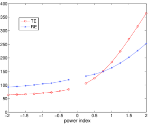
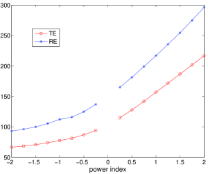
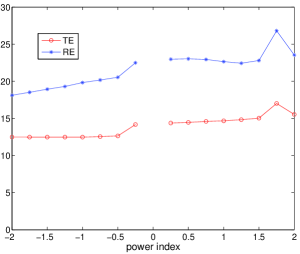
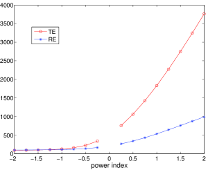
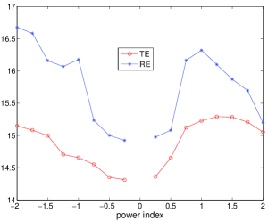
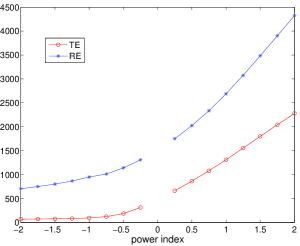
The TE criteria of the recursive training data are shown from Fig. 1 to Fig. 6. The relationship of TE criteria and the corresponding RE criterion with same index of powLSE are shown in Fig. 7 – Fig. 12. And, the RE values of MLE, LogLSE and powLSE with optimal index are listed in Table 7.

Figure 1: TE values of NTDS with MLE, LogLSE and powLSE.

Figure 2: TE values of JDM–I with MLE, LogLSE and powLSE.

Figure 3: TE values of JDM–II with MLE, LogLSE and powLSE.

Figure 4: TE values of JDM–III with MLE, LogLSE and powLSE.

Figure 5: TE values of JDM–IV with MLE, LogLSE and powLSE.

Figure 6: TE values of AT& T with MLE, LogLSE and powLSE.

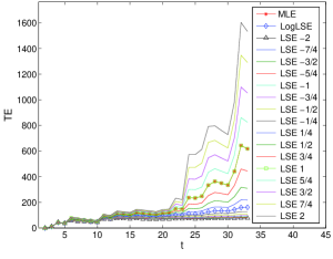
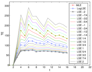
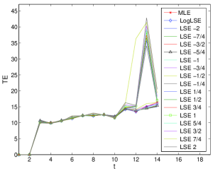
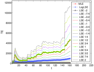
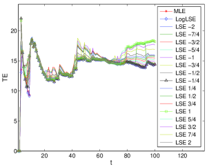
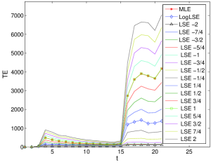
From Fig.1 to Fig.6, we can conclude that the TE of powLSE with optimal index along the segmentation data can achieve relatively small value compared to MLE and LogLSE. From Fig.7 – Fig.12, we can see that the predictive RE values and the TE values in training data are also similar, hence it demonstrates that the optimization of power index is reasonable.

Figure 7: RE and TE values of NTDS by powLSE with different power index.

Figure 8: RE and TE values of JDM–I by powLSE with different power index.

Figure 9: RE and TE values of JDM–II by powLSE with different power index.

Figure 10: RE and TE values of JDM–III by powLSE with different power index.

Figure 11: RE and TE values of JDM–IV by powLSE with different power index.

Figure 12: RE and TE values of AT& T by powLSE with different power index.

Table 7: The RE evaluation of MLE, LSE,LogLSE and powLSE. (%)

FNLSE	NTDS	JDM–I	JDM–II	JDM–III	JDM–IV	AT & T
MLE	162.829	216.609	21.677	536.269	16.043	2680.787
LSE	163.482	216.888	22.650	535.191	16.320	2688.571
LogLSE	125.966	150.135	21.224	208.453	16.230	1511.177
powLSE opt	92.476	93.177	19.305	101.031	14.922	706.623
$\hat{\alpha}$	-2	-2	-5/4	-2	-1/4	-2
powLSE best	92.476	93.177	18.122	101.031	14.922	706.623
$\hat{\alpha}$	-2	-2	-2	-2	-1/4	-2

As powLSE with $\alpha=1$ is the traditional LSE, the simulation results are also listed in the Table 7 for comparison. The RE evaluation results with MLE, LogLSE and powLSE with optimal index in Table 7, the simulation results show that powLSE with the optimal index can outperform the MLE, LSE and LogLSE according to RE criterion. And, both powLSE with optimal index and LogLSE outperform the traditional LSE and MLE.

4.2.2 Experimental Results with Braun statistic criterion

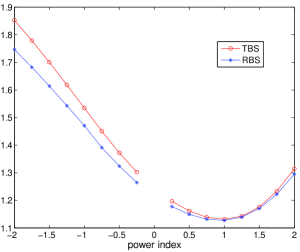
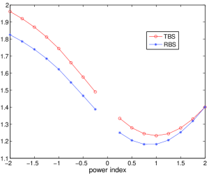
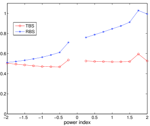
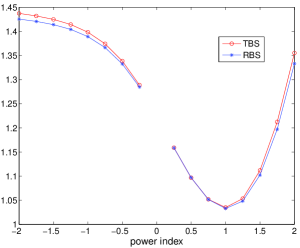
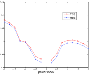
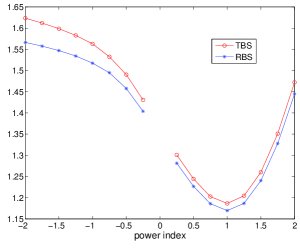
The TBS criteria of the recursive training data are shown from Fig. 13 to Fig. 18, the corresponding one–step–ahead recursive prediction RBS criteria are shown from Fig. 19 – Fig. 24. And the RBS values of MLE, LogLSE and powLSE with optimal index are listed in Table 8.

Figure 13: TBR values of NTDS with MLE, LogLSE and powLSE.

Figure 14: TBR values of JDM–I with MLE, LogLSE and powLSE.

Figure 15: TBR values of JDM–II with MLE, LogLSE and powLSE.

Figure 16: TBR values of JDM–III with MLE, LogLSE and powLSE.

Figure 17: TBR values of JDM–IV with MLE, LogLSE and powLSE.

Figure 18: TBR values of AT& T with MLE, LogLSE and powLSE.

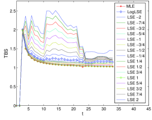
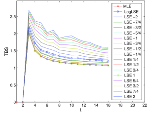
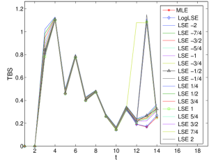
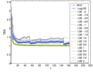
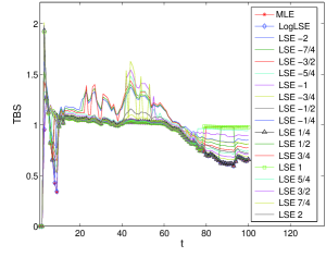
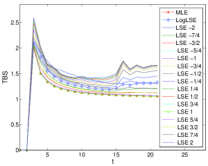
From Fig. 13 to Fig. 18, we can conclude that powLSE with optimal index can achieve relatively smaller profiles than MLE, LSE ad LogLSE. And, Fig. 19 –Fig. 24 manifest the validation of power index optimization with Braun statistic criterion.

Figure 19: RBS and TBS values of NTDS by powLSE with different power index.

Figure 20: RBS and TBS values of JDM–I by powLSE with different power index.

Figure 21: RBS and TBS values of JDM–II by powLSE with different power index.

Figure 22: RBS and TBS values of JDM–III by powLSE with different power index.

Figure 23: RBS and TBS values of JDM–IV by powLSE with different power index.

Figure 24: RBS and TBS values of AT& T by powLSE with different power index.

Table 8: The Braun statistic evaluation of LSE,LogLSE and powLSE. (%)

FNLSE	NTDS	JDM–I	JDM–II	JDM–III	JDM–IV	AT & T
MLE	1.124	1.182	0.657	1.033	0.955	1.170
LSE	1.128	1.183	0.847	1.033	0.994	1.170
LogLSE	1.216	1.313	0.653	1.225	0.963	1.342
powLSE opt	1.128	1.183	0.612	1.033	0.918	1.170
$\hat{\alpha}$	1	1	-1/2	1	1/4	1
powLSE best	1.128	1.182	0.512	1.033	0.918	1.170
$\hat{\alpha}$	1	3/4	-2	1	1/4	1

From the RBS evaluation values in Table 8, we can see that powLSE with optimal index outperforms LSE on data set JDM–II and JDM–IV, and has same performances comparing with LSE on the other four data sets. It demonstrates that powLSE extends LSE according to Braun statistic criterion.

4.2.3 Heteroscedasticity of data

All of the corresponding variances with original data and residual data predicted by MLE, LSE ,LogLSE and powLSE with optimal index are shown in Fig. 25 – Fig. 30, where we denote the powLSE optimized by RE criterion as powLSE RE, and denote the powLSE optimized by Braun statistic criterion as powLSE BS.

Figure 25: Variances of NTDS with MLE, LogLSE and powLSE.

Figure 26: Variances of JDM–I with MLE, LogLSE and powLSE.

Figure 27: Variances of JDM–II with MLE, LogLSE and powLSE.

Figure 28: Variances of JDM–III with MLE, LogLSE and powLSE.

Figure 29: Variances of JDM–IV with MLE, LogLSE and powLSE.

Figure 30: Variances of AT& T with MLE, LogLSE and powLSE.

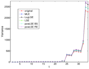
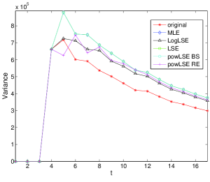
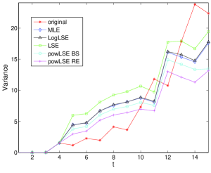
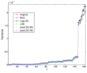
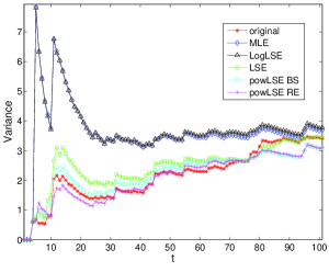
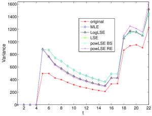
We can conclude from Fig. 25 to Fig. 30 that all of the six failure data have heteroscedasticity along the time, the JDM–II and JDM–IV, which have relatively small variance values, have small predictive RE values (see Table 7), and the variance change points reflect the role of sample data affecting the deviation at the same time. And, the heteroscedasticity provides the information of data sensitivity to modeling software reliability. All of the information would provide help for statistical modeling and explanation for bad performance.

5 Conclusion

A FNLSE framework is proposed, two of special cases, LogLSE and powLSE, are applied to the parameter estimation of Jelinski–Moranda model. It extends the LSE and LogLSE in software reliability and possesses the data compressing role with the proper selection of transformation function, and it is proved as a weighted LSE. Our motivation and modeling procedure are different from famous Box–Cox transformation. It is also treated as a general model to discuss statistical data analysis with non–normality and heteroscedasticity. Furthermore, the LogLSE and powLSE of Jelinski–Moranda model are discussed and derived. Their prediction accuracies are evaluated by two statistical indexes relative error and Braun statistic. The simulation results demonstrate that both powLSE and LogLSE outperform MLE and LSE of Jelinski–Moranda model, and powLSE outperforms LogLSE with the optimal indexes. The future work will focus on the simulation evaluation on more failure data sets with FNLSE, compare the performance of FNLSE with time–dependent model, and apply the FNLSE to the other software reliability models to generalize the estimation algorithm modeled by LSE.

6 Acknowledgements

The research was partially supported by 863 Project of China (2008AA02Z306), Beihang SRSA Program under grant No. 2006-49-8-4, and NSFC(10801019),

References

- [1] Musa, J.D., Iannino, A., Okumoto, K., 1987. Software Reliability: Measurement, Prediction, Application. New York: McGraw- Hill.
- [2] Jelinski, Z., Moranda, P.B., 1972. Software reliability research. in Statistical Computer Performance Evaluation (W. Freiberger ed.).Academic Press, 465–484.
- [3] Schafer, R.E., Alter, J.F., Angus, J.E., Emoto, S.E., 1979. Validation of Software Reliability Models. Rome Air Development Center, Technical Report RADC–TR–79–147, Rome, NY.
- [4] Lyu, M.R. 1996, Handbook of Software Reliability Engineering. IEEE Computer Society Press and McGraw-Hill Book Company.
- [5] Cai, K.Y., 1998a. Software defect and operational profile modeling, Kluwer Academic Publishers, Norwell, MA.
- [6] Huang, X.Z., 2002. Software Reliability, Safety and Quality Assurance. Beijing: Electronic Industry Press. (in Chinese)
- [7] Littlewood, B., Sofer, A., 1987. A Bayesian modification to the Jelinski-Moranda software reliability growth model. Software Engineering Journal. 2(2), 30-41.
- [8] Pham, L., Pham, H., 2000. Software reliability models with time-dependent hazard function based on Bayesian approach. IEEE Transactions on Systems, Man, and Cybernetics, Part A, 30(1), 25-35.
- [9] Bai, C.G., Hu, Q.P., Xie, M., Ng, S.H., 2005. Software failure prediction based on Markov Bayesian network model. The Journal of Systems and Software. 74(3), 275-282.
- [10] Cai, K.Y., Cai, L., Wang, W.D., Yu, Z.Y., Zhang, D., 2001. On the neural network approach in software reliability modeling. The Journal of Systems and Software, 58(1), 47-62.
- [11] Su, Y.S., Huang, C.Y., 2007. Neural-network-based approaches for software reliability estimation using dynamic weighted combinational models. The Journal of Systems and Software. 80(4), 606-615.
- [12] Hong, W.C., Pai, P.F., 2006a. Predicting Engine Reliability by Support Vector Machines. International Journal of Advanced Manufacturing Technology, 28(1-2), 154-161.
- [13] Pai, P.F., Hong, W.C., 2006b. Software reliability forecasting by support vector machines with simulated annealing algorithms. 79(6), 747–755.
- [14] Raj Kiran, N., Ravi, V., 2007. Software Reliability Prediction using Wavelet Neural Networks . International Conference on Computational Intelligence and Multimedia Applications. 195–199.
- [15] Vinay Kumar, K., Ravi, V., Carr, M., Raj Kiran, N., 2008. Software development cost estimation using wavelet neural networks. The Journal of Systems and Software. 81(11), 1853-1867.
- [16] Cai, K.Y., 1998b. On Estimating the Number of Defects Remaining in Software. Journal of Systems and Software, 40(2), 93-114.
- [17] Liu, J.W., Hu, Y.B., Wang X.L., Xu M.Z., 2008. Novel Nonlinear Least Square Parameter Estimation Method for Jelinski-Moranda Model. Journal of System Simulation. 20(18), 4791–4794.
- [18] Marquardt, D.W., 1963. An Algorithm for Least-Squares Estimation of Nonlinear Parameters. Journal of the Society for Industrial and Applied Mathematics. 11(2), 431–441 .
- [19] Barham R.H., Drane W.,1972. An Algorithm for Least Squares Estimation of Nonlinear Parameters When Some of the Parameters Are Linear. Technometrics. 14(3), 757–766.
- [20] Bjrck, A., 1996. Numerical Methods for Least Squares Problems. SIAM Press, Philadelphia, USA.
- [21] Pindyck, R.S., Rubinfeld D.L., 2005. Econometric Models and Economic Forecasts (4th Edition). China Machine Press, Beijing.
- [22] Briand, L.C., Basili, V.R., Thomas W.M., 1992. A Pattern Recognition Approach for Software Engineering Data Analysis. IEEE Transactions on Software Engineering. 18(11), 931–942.
- [23] He, S.Y., 2004. Applied Time Series Analysis. Peking Univeristy Press,Beijing.
- [24] Box, G.E.P., Cox, D.R..,1964. An Analysis of Transformations. Journal of the Royal Statistical Society. Series B (Methodological). 26(2), 211–252.
- [25] Marazzi, A., Yohai, V., 2004. Robust Box CCox transformations for simple regression. In: Hubert, M., Pison, G., Struyf, A., Van Aelst, S. (Eds.), Theory and Applications of Recent Robust Methods. I: Statistics for Industry and Technology, 173 C182.
- [26] Goldfeld S.M., Quandt R. E., 1965. Some Tests for Homoscedasticity. Journal of the American Statistical Society, 60(310), 539-547.
- [27] Markovi, D., Juki, D., Beni ,M., 2009. Nonlinear weighted least squares estimation of a three-parameter Weibull density with a nonparametric start. Journal of Computational and Applied Mathematics. 228(1), 304–312.
- [28] Ramsay, J.O., Silverman, B.W., 2006. Functional Data Analysis (second edition). Science Press, Beijing.
- [29] Zhu, L.X., Zhu, L.P. , Li, X., 2007. Transformed Partial Least Squares for Multivariate Data. Statistica Sinica. 17(4), 1657-1675.
- [30] Peng, L., Yao, Q.W., 2003. Least absolute deviations estimation for ARCH and GARCH models. Biometrika, 90(4), 967-975.
- [31] Patrick Koh, S.L., 2008. Weighted Least-Square Estimate for Software Error Intensity. Journal of the Chinese Institute of Industrial Engineers. 25(2), 162-173.
- [32] Hopkins,W.G., 2003. Log Transformation. In: A New View of Statistics, http://www.sportsci.org/ resource/ stats/ logtrans.html. Accessed 1 July 2010.
- [33] Gujarati, D.N.,2004. Basic econometrics. McGraw-Hill, New York.
- [34] Musa, J.D., 1979. Software reliability data, IEEE Computer Society- Repository.
- [35] Cai, K.Y., 1995. Elements of Software Reliability Engineering. Tsinghua University Press , Beijing.