A Storm in a “T” Cup

Abstract

We revisit the process of transversification and agglomeration of particle momenta that are often performed in analyses at hadron colliders, and show that many of the existing mass-measurement variables proposed for hadron colliders are far more closely related to each other than is widely appreciated, and indeed can all be viewed as a common mass bound specialized for a variety of purposes.

1 Transversification and Agglomeration

Almost every analysis of data from hadron colliders uses at some point a variable which represents a “projection” of an energy or momentum into the plane transverse to the beams (see Barr:2010zj ; Barr:2011xt for recent reviews.). The typical reason for performing these projections is that one does not wish the analysis to be sensitive to the unknown momentum. When it comes to projecting geometric 3-vectors like $\vec{P}$, the decomposition $\vec{P}\equiv\left(\vec{p}_{T},p_{z}\right)$ is unambiguous. One has no other choice – the very definition of the transverse plane requires one simply to dispose of the $z$-component to arrive at $\vec{p}_{T}=\left(p_{x},p_{y}\right)$. However, “projecting” the time-like component $E$ is not a well defined operation. There is not a single correct answer, but rather a number of different answers, each with different properties and motivations. How one should (and even whether one should) project time-like components of (1+3) Lorentz vectors is dependent on what one is trying to achieve. In the particle physics literature, one can find evidence of at least three different types of “transverse projection” being applied to (1+3)-Lorentz vectors (summarized in Table 1), although this diversity is not obvious at first glance, as the majority of papers do not explicitly state which projection they are using Barr:2011xt .

	Transverse projection method
Quantity	Mass-preserving ‘$\top$’	Speed-preserving ‘$\vee$’	Massless ‘${\circ}$’
Original (4)-momentum	$P^{\mu}=\left(E,\vec{p}_{T},p_{z}\right)$
(1+3)-mass invariant	$M=\sqrt{E^{2}-\vec{p}_{T}^{\,2}-p_{z}^{2}}$
Transverse momentum	$\vec{p}_{T}\equiv\left(p_{x},p_{y}\right)$
(1+2)-vectors	$p_{\top}^{\alpha}\equiv\left(e_{\top},\vec{p}_{\top}\right)$	$p_{\vee}^{\alpha}\equiv\left(e_{\vee},\vec{p}_{\vee}\right)$	$p_{\circ}^{\alpha}\equiv\left(e_{\circ},\vec{p}_{\circ}\right)$
Transverse momentum under the projection	$\vec{p}_{\top}\equiv\vec{p}_{T}$	$\vec{p}_{\vee}\equiv\vec{p}_{T}$	$\vec{p}_{\circ}\equiv\vec{p}_{T}$
Transverse energy under the projection	$e_{\top}\equiv\sqrt{M^{2}+\vec{p}_{T}^{\,2}}$	$e_{\vee}\equiv E\left|{\sin\theta}\right|=|\vec{p}_{T}|/V$	$e_{\circ}\equiv|\vec{p}_{T}|$
Transverse mass under the projection	$m_{\top}^{2}=e_{\top}^{2}-\vec{p}_{\top}^{\,2}$	$m_{\vee}^{2}\equiv e_{\vee}^{2}-\vec{p}_{\vee}^{\,2}$	$m_{\circ}^{2}\equiv e_{\circ}^{2}-\vec{p}_{\circ}^{\,2}=0$
Relationship between transverse quantity and its (1+3) analogue	$m_{\top}=M$	$m_{\vee}=M\left|\sin\theta\right|$	$m_{\circ}=0$
	$\frac{1}{v_{\top}}=\frac{1}{V}\sqrt{1+(1-V^{2})\frac{p_{z}^{2}}{p_{T}^{2}}}$	$v_{\vee}=V$	$v_{\circ}=1$
Equivalence classes under $(1+3)\stackrel{{\scriptstyle\mathrm{proj}}}{{\longmapsto}}(1+2)$	All $P^{\mu}$ with the same $p_{x}$, $p_{y}$ and $M$	All $P^{\mu}$ with the same $p_{x}$, $p_{y}$ and $V$	All $P^{\mu}$ with the same $p_{x}$ and $p_{y}$

Table 1: A comparison of the three transversification methods.

In forming transverse kinematic variables for composite particles, one needs to perform two separate operations: summation of the momentum vectors of the daughter particles, and projecting into the transverse plane. The order of these operations does not matter for the two space-like vector components. However, projecting before or after the sum can make a very significant difference to the value of the time-like component of the final (1+2) vector (i.e., $e_{\top}$, $e_{\vee}$ or $e_{\circ}$ in Table 1) – and therefore the operations of projecting and summing do not generally commute:

2 Interpretation and Generalization

We define the general procedure that can be used to construct the mass-bound variables. We describe a broad class of such variables, where each individual variable $M_{\{indices\}}$ will be labelled by a certain set of indices $\{indices\}$ indicative of the way the particular variable was constructed, namely:

• We are targeting the general event topology, where we imagine the inclusive production of $N$ parents, each one of our variables will necessarily carry a corresponding index $N$. In the process of constructing such a variable, we will have to partition (and then agglomerate) the observed visible particles in the event into $N$ groups ${\cal V}_{a}$, $(a=1,2,\ldots,N)$. We will then form the (1+3) dimensional invariant mass of each parent ${\mathbb{P}_{a}}$

  $${\cal M}_{a}\equiv\sqrt{g_{\mu\nu}\,({\mathbf{P}}_{a}^{\mu}+{\mathbf{Q}}_{a}^{\mu})({\mathbf{P}}^{\nu}_{a}+{\mathbf{Q}}^{\nu}_{a})},$$ (1)

  which is constructed out of the (1+3) momenta ${\mathbf{P}}^{\mu}_{a}$ and ${\mathbf{Q}}^{\mu}_{a}$ of the visible and invisible composite daughter particles, respectively.

• Optionally, instead of the (1+3) dimensional parent mass (1), we may choose to consider the corresponding early-partitioned (late-projected) transverse mass or the late-partitioned (early-projected) transverse mass

  $${\cal M}_{aT}\equiv\sqrt{g_{\alpha\beta}\,({\mathbf{p}}_{aT}^{\alpha}+{\mathbf{q}}_{aT}^{\alpha})({\mathbf{p}}^{\beta}_{aT}+{\mathbf{q}}^{\beta}_{aT})},~{}~{}~{}~{}~{}~{}~{}~{}{\cal M}_{Ta}\equiv\sqrt{g_{\alpha\beta}\,({\mathbf{p}}_{Ta}^{\alpha}+{\mathbf{q}}_{Ta}^{\alpha})({\mathbf{p}}^{\beta}_{Ta}+{\mathbf{q}}^{\beta}_{Ta})},$$ (2)

  where ${\mathbf{p}}^{\alpha}_{aT}$, ${\mathbf{p}}^{\alpha}_{Ta}$, ${\mathbf{q}}^{\alpha}_{aT}$ and ${\mathbf{q}}^{\alpha}_{Ta}$ are the (1+2) dimensional momentum vectors for visible and invisible sectors before and after partitioning, and the index $T$ takes values in $\left\{\top,\vee,{\circ}\right\}$, as described in Table 1.

• The last step is to consider the largest hypothesized parent mass ($\max\left[{\cal M}_{a}\right]$, $\max\left[{\cal M}_{aT}\right]$ or $\max\left[{\cal M}_{Ta}\right]$ as appropriate) and minimize it over all possible values of the unknown invisible momenta consistent with the constraints. This minimization is always a well-defined, unambiguous operation, which yields a unique numerical answer Konar:2008ei ,

  $$M_{N}\equiv\min_{\begin{subarray}{c}\sum\vec{q}_{iT}=\not{\vec{p}}_{T}\end{subarray}}\left[\max_{a}\left[{\cal M}_{a}\right]\right],~{}~{}~{}~{}~{}~{}M_{NT}\equiv\min_{\begin{subarray}{c}\sum\vec{q}_{iT}=\not{\vec{p}}_{T}\end{subarray}}\left[\max_{a}\left[{\cal M}_{aT}\right]\right],~{}~{}~{}~{}~{}~{}M_{TN}\equiv\min_{\begin{subarray}{c}\sum\vec{q}_{iT}=\not{\vec{p}}_{T}\end{subarray}}\left[\max_{a}\left[{\cal M}_{Ta}\right]\right]\,.$$ (3)

  The minimization over the unknown parameter is performed in order to guarentee that the resultant variable cannot be larger than the mass of the heaviest parent, resulting in an event-by-event lower bound on the mass of the heaviest parent.

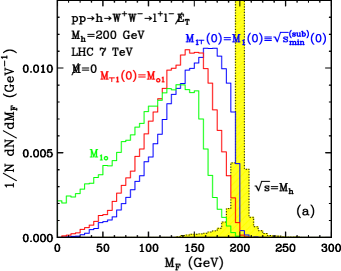
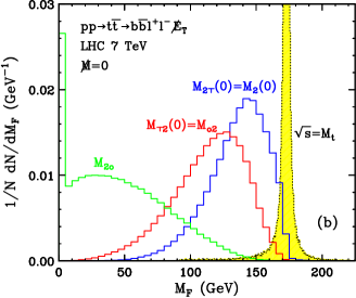
We emphasize that these variables turn out not to be a function of the individual invisible mass hypothesis, but instead turn out to be a function of the set, ${\not{{\mathbf{M}}}}=\left\{{{\not{{\mathbf{M}}}}_{a}}\mid{a\in\mathcal{P}}\right\}$, containing the $N$ “invisible mass-sum parameters, ${\not{{\mathbf{M}}}}_{a}$” defined by ${\not{{\mathbf{M}}}}_{a}\equiv\sum_{i\in{\mathcal{I}_{a}}}\tilde{M}_{i}$. These mass parameters are simple arithmetic sums of the hypothesized masses of the individual invisible particles associated with any given parent ${\mathbb{P}_{a}}$. One can also prove from above minimization that the early - agglomerated (late projected) “’transverse” variables are “secretly” (1+3) dimensional, $M_{N\top}({\not{{\mathbf{M}}}})=M_{N}({\not{{\mathbf{M}}}})$. This identity reveals that “transverse” quantities do not necessarily “forget” about relative longitudinal momenta. In particular, this relation teaches us that whenever the composite particles are formed before the transverse projection, the information about the relative longitudinal momenta is retained, and the result is the same as if everything was done in (1+3) dimensions throughout. As a result, $M_{N\top}$ automatically inherits all the advantages and disadvantages of its (1+3) cousin $M_{N}$. These basic variables ( “unprojected” $M_{N}$ and the “singly projected” $M_{NT}$ and $M_{TN}$ variables) are shown in Fig. 1 for some examples. This basic set of variables can be further extended, by considering a second level of projections within the transverse plane Barr:2010zj ; Konar:2009wn .

The guiding principle we employ for creating useful hadron-collider event variables, is that: we should place the best possible bounds on any Lorentz invariants of interest, where it is not possible to determine the actual values of those Lorentz invariants due to incomplete event information. Such incomplete information could take the form of lack of knowledge of the longitudinal momentum of the primary collision, or lack of knowledge of the 4-momenta of individual invisible particles, or lack of knowledge of the number of invisible particles which were present, etc. We contrast this principle with the alternative approach that is used to motivate event variables without any explicit regard to whether they have an interpretation as an optimal bound of a Lorentz invariant. This alternative approach tends to recommend the use of variables that are somewhat ad-hoc, but by construction possess useful invariances (such as invariance under longitudinal boosts) which are designed to remove sensitivity to quantities that are unknown. Examples are $\not{\vec{p}}_{T}$, $h_{T}$ and $m_{\mathrm{eff}}$. A careful study of similarities and differences of these mass-bound variables not only gives insights into why (and under what circumstances) these choices are appropriate, it also fits them into a common framework – from which it is straightforward to make generalizations to more complex decay topologies. Well known kinematic variables such as $M_{T2}$ Barr:2010zj ; Lester:1999tx ; Barr:2003rg ; Burns:2008va and $\sqrt{s}_{min}$ Konar:2008ei ; Konar:2010ma are a special case of the mass-bound variables.

         

Figure 1: (a) Unit-normalized distribution of the five $N=1$ mass-bound variables $M_{{\cal F}}$, ${{\cal F}}\in\{1,1\top,\top 1,1{\circ},{\circ}1\}$ for the inclusive Higgs production process $h\to W^{+}W^{-}\to\ell^{+}\ell^{-}+\not{p}_{T}$ at a 7 TeV LHC, with $m_{h}=200$ GeV and ${\not{{\mathbf{M}}}}=0$. The dotted (yellow-shaded) histogram gives the true $\sqrt{\hat{s}}$ distribution, which in this case is given by the Breit-Wigner $h$ resonance. (b) The unprojected $M_{2}$ and the singly projected variables $M_{2\top}$, $M_{\top 2}$, $M_{{\circ}2}$ and $M_{2{\circ}}$ for $N=2$ and $t\bar{t}$ example.

References

- (1) A. J. Barr, C. G. Lester, J. Phys. G G37, 123001 (2010). [arXiv:1004.2732 [hep-ph]].
- (2) A. J. Barr, T. J. Khoo, P. Konar, K. Kong, C. G. Lester, K. T. Matchev, M. Park, [arXiv:1105.2977 [hep-ph]].
- (3) P. Konar, K. Kong, K. T. Matchev, JHEP 0903, 085 (2009). [arXiv:0812.1042 [hep-ph]].
- (4) P. Konar, K. Kong, K. T. Matchev, M. Park, Phys. Rev. Lett. 105, 051802 (2010). [arXiv:0910.3679 [hep-ph]].
- (5) C. G. Lester, D. J. Summers, Phys. Lett. B463, 99-103 (1999). [hep-ph/9906349].
- (6) A. Barr, C. Lester, P. Stephens, J. Phys. G G29, 2343-2363 (2003). [hep-ph/0304226].
- (7) M. Burns, K. Kong, K. T. Matchev, M. Park, JHEP 0903, 143 (2009). [arXiv:0810.5576 [hep-ph]].
- (8) P. Konar, K. Kong, K. T. Matchev, M. Park, JHEP 1106, 041 (2011). [arXiv:1006.0653 [hep-ph]].