Zeros and ratio asymptotics for matrix orthogonal polynomials

Abstract

Ratio asymptotics for matrix orthogonal polynomials with recurrence coefficients $A_{n}$ and $B_{n}$ having limits $A$ and $B$ respectively (the matrix Nevai class) were obtained by Durán. In the present paper we obtain an alternative description of the limiting ratio. We generalize it to recurrence coefficients which are asymptotically periodic with higher periodicity, and/or which are slowly varying in function of a parameter. Under such assumptions, we also find the limiting zero distribution of the matrix orthogonal polynomials, generalizing results by Durán-López-Saff and Dette-Reuther to the non-Hermitian case. Our proofs are based on ‘normal family’ arguments and on the solution to a quadratic eigenvalue problem. As an application of our results we obtain new explicit formulas for the spectral measures of the matrix Chebyshev polynomials of the first and second kind, and we derive the asymptotic eigenvalue distribution for a class of random band matrices generalizing the tridiagonal matrices introduced by Dumitriu-Edelman.

Keywords: matrix orthogonal polynomial, (block) Jacobi matrix, recurrence coefficient, (locally) block Toeplitz matrix, ratio asymptotics, limiting zero distribution, quadratic eigenvalue problem, normal family, matrix Chebyshev polynomial, random band matrix.

1 Introduction

Let $(P_{n}(x))_{n=0}^{\infty}$ be a sequence of matrix-valued polynomials of size $r\times r$ ($r\geq 1$) generated by the recurrence relation

$$xP_{n}(x)=A_{n+1}P_{n+1}(x)+B_{n}P_{n}(x)+A_{n}^{*}P_{n-1}(x),\qquad n\geq 0,$$ (1.1)

with initial conditions $P_{-1}(x)\equiv 0\in\mathbb{C}^{r\times r}$ and $P_{0}(x)\equiv I_{r},$ with $I_{r}$ the identity matrix of size $r$. The coefficients $A_{k}$ and $B_{k}$ are complex matrices of size $r\times r$. We assume that each matrix $A_{k}$ is nonsingular and $B_{k}$ is Hermitian. The star superscript denotes the Hermitian conjugation.

The polynomials generated by (1.1) satisfy orthogonality relations with respect to a matrix-valued measure (spectral measure) on the real line (Favard’s theorem [8]) and they are therefore called matrix orthogonal polynomials. The study of such polynomials goes back at least to [19] and we refer to the survey paper [8] for a detailed discussion of the available literature and for many more references. Some recent developments and applications of matrix orthogonal polynomials can be found in [4, 6, 9, 17] among many others.

To the recurrence (1.1) we associate the block Jacobi matrix

$$J_{n}=\begin{pmatrix}B_{0}&A_{1}&&&0\\ A_{1}^{*}&B_{1}&A_{2}\\ &A_{2}^{*}&\ddots&\ddots\\ &&\ddots&\ddots&A_{n-1}\\ 0&&&A_{n-1}^{*}&B_{n-1}\end{pmatrix}_{rn\times rn},$$ (1.2)

which is a Hermitian, block tridiagonal matrix. It is well-known that

$$\det P_{n}(x)=c_{n}\det(xI_{n}-J_{n})$$

with $c_{n}=\det(A_{n}^{-1}\cdots A_{2}^{-1}A_{1}^{-1})\neq 0$, see [8, 14], and with the zeros of the matrix polynomial $P_{n}(x)$ we mean the zeros of the determinant $\det P_{n}(x)$, or equivalently the eigenvalues of the matrix $J_{n}$ defined in (1.2) (counting multiplicities).

The polynomials $(P_{n}(x))_{n=0}^{\infty}$ are said to belong to the matrix Nevai class if the limits

$$\lim_{n\to\infty}A_{n}=A,\qquad\lim_{n\to\infty}B_{n}=B,$$ (1.3)

exist, where we will assume throughout this paper that $A$ is nonsingular.

One of the famous classical results on orthogonal polynomials is Rakhmanov’s theorem [25], see [1, 9, 28] for a survey of the recent advances in this direction. Rakhmanov’s theorem for matrix orthogonal polynomials on the real line is discussed in [9, 30]. These results give a sufficient condition on the spectral measure of the matrix orthogonal polynomials, in order to have recurrence coefficients in the matrix Nevai class, with limiting values $A=I_{r}$ and $B=0$. For a discussion of the matrix Nevai class in this case, see [18].

Durán [13] shows that in the matrix Nevai class (1.3), the limiting matrix ratio

$$R(x):=\lim_{n\to\infty}P_{n}(x)P_{n+1}^{-1}(x),\qquad x\in\mathbb{C}\setminus[-M,M],$$ (1.4)

exists and depends analytically on $x\in\mathbb{C}\setminus[-M,M]$. Here $M>0$ is a constant such that all the zeros of all the matrix polynomials $P_{n}(x)$ are in $[-M,M]$. Moreover, it is also proved in [13] that $R(x)A^{-1}$ is the Stieltjes transform of the spectral measure for the matrix Chebyshev polynomials of the second kind generated by the constant recurrence coefficients $A$ and $B$; see Section 4.

The present paper has several purposes. First we will give a different formulation of Durán’s result on ratio asymptotics [13]. In particular we will give a self-contained proof of the existence of the limiting ratio $R(x)$ and express it in terms of a quadratic eigenvalue problem. Second, our approach can also be used to obtain ratio asymptotics for some extensions to the matrix Nevai class. More precisely, we will allow the coefficients $A_{n}$ and $B_{n}$ to be slowly varying in function of a parameter, or to be asymptotically periodic with higher periodicity. In both cases we prove the existence of the limiting ratio (the limit may be local or periodic) and give an explicit formula for it.

To prove these results we will work with normal families in the sense of Montel’s theorem. Similar arguments can be found at various places in the literature and our approach will be based in particular on the work by Kuijlaars-Van Assche [22] and its further developments in [3, 7, 11, 20]. We point out that an alternative approach for obtaining ratio asymptotics, is to use the generalized Poincaré theorem (see [24, 27] for this theorem); but the normal family argument has the advantage that it also works for slowly varying recurrence coefficients; see Section 3.1 for more details.

The third purpose of the paper is to obtain a new description of the limiting zero distribution of the matrix polynomials $(P_{n}(x))_{n=0}^{\infty}$. Durán-López-Saff [15] showed that in the matrix Nevai class (1.3), and assuming that $A$ is Hermitian, then the zero distribution of $P_{n}(x)$ has a limit for $n\to\infty$ in the sense of the weak convergence of measures. They expressed the limiting zero distribution of $P_{n}(x)$ in terms of the spectral measure for the matrix Chebyshev polynomials of the first kind, see Section 5 for the details. In contrast to the work of [15] the results derived in the present paper are also applicable in the case when the matrix $A$ is nonsingular but not necessarily Hermitian. Maybe not surprisingly, the limiting eigenvalue distribution of the matrix $J_{n}$ in (1.2)–(1.3) is the same as the limiting eigenvalue distribution for $n\to\infty$ of the block Toeplitz matrix

$$T_{n}=\begin{pmatrix}B&A&&&0\\ A^{*}&B&A\\ &A^{*}&\ddots&\ddots\\ &&\ddots&\ddots&A\\ 0&&&A^{*}&B\end{pmatrix}_{rn\times rn}.$$ (1.5)

The eigenvalue counting measure of the matrix $T_{n}$ has a weak limit for $n\to\infty$ [29] and a description of the limiting measure can be obtained from [5, 10, 29].

In this paper we establish the limiting zero distribution of the matrix polynomials $P_{n}(x)$ as a consequence of our results on ratio asymptotics. We also find the limiting zero distribution for the previously mentioned extensions to the matrix Nevai class. That is, the coefficients $A_{n}$ and $B_{n}$ are again allowed to be slowly varying in function of a parameter, or to be asymptotically periodic with higher periodicity.

Incidentally, we mention that it is possible to devise an alternative, linear algebra theoretic proof for the fact that the matrices $J_{n}$ and $T_{n}$ have the same weak limiting eigenvalue distribution, using the fact that the block Jacobi matrix (1.2) is Hermitian [21]; however our approach has the advantage that it can be also used in the non-Hermitian case, at least in principle. This means that most of the methodology derived in this paper is also applicable in the case when the recurrence matrix (1.2) generating the polynomials $P_{n}(x)$, is no longer Hermitian, or when it has a larger band width in its block lower triangular part, as in [3]. In fact the key places where we use the Hermiticity are in the proof of Proposition 2.1 and in the proof of Lemma 7.1, see [11]; but it is reasonable to expect that both facts remain true for some specific non-Hermitian cases as well. This may be an interesting topic for further research.

The remaining part of this paper is organized as follows. In the next section we state our results for the case of the matrix Nevai class. In Section 3 we generalize these findings, to the context of recurrence coefficients with slowly varying or asymptotically periodic behavior. In Section 4 we apply our results to find new formulas for the spectral measures of the matrix Chebyshev polynomials of the first and second kind. In Section 5 we relate our formula for the limiting zero distribution to the one of Durán-López-Saff [15]. In Section 6 we indicate some potential applications in the context of random matrices. In particular we derive the limiting eigenvalue distribution for a class of random band matrices, which generalize the random tridiagonal representations of the $\beta$-ensembles, which were introduced in [12]. Finally, Section 7 contains the proofs of the main results.

2 Statement of results: the matrix Nevai class

2.1 The quadratic eigenvalue problem

Throughout this section we work in the matrix Nevai class (1.2)–(1.3). Observe that the limiting ratio $R(x)$ in (1.4) satisfies the matrix relation

$$A^{*}R(x)+B-xI_{r}+AR^{-1}(x)=0,\qquad x\in\mathbb{C}\setminus[-M,M],$$ (2.1)

which is an easy consequence of the three term recurrence (1.1). For a simple motivation of our approach we assume at the moment that for each $x\in\mathbb{C}\setminus[-M,M]$, the matrix $R(x)$ is diagonalizable with distinct eigenvalues $z_{k}=z_{k}(x)$, $k=1,\ldots,r$. Let $\mathbf{v}_{k}(x)\in\mathbb{C}^{r}$ be the corresponding eigenvectors so that

$$R(x)\mathbf{v}_{k}(x)=z_{k}(x)\mathbf{v}_{k}(x),$$

for $k=1,\ldots,r$. Multiplying (2.1) on the right with $\mathbf{v}_{k}(x)$ we find the relation

$$\left(z_{k}(x)A^{*}+B-xI_{r}+z_{k}^{-1}(x)A\right)\mathbf{v}_{k}(x)=\mathbf{0},$$ (2.2)

where $\mathbf{0}$ denotes a column vector with all its entries equal to zero. This relation implies in particular that

$$\det\left(z_{k}(x)A^{*}+B-xI_{r}+z_{k}^{-1}(x)A\right)=0.$$ (2.3)

We can view (2.3) as a quadratic eigenvalue problem in the variable $z=z_{k}(x)$, and it gives us an algebraic equation for the eigenvalues of the limiting ratio $R(x)$. The corresponding eigenvectors $\mathbf{v}_{k}(x)$ can then be found from (2.2). Note that the equation (2.3) has $2r$ roots $z=z_{k}(x)$, $k=1,\ldots,2r$. Ordering these roots by increasing modulus

$$0<|z_{1}(x)|\leq|z_{2}(x)|\leq\ldots\leq|z_{r}(x)|\leq|z_{r+1}(x)|\leq\ldots\leq|z_{2r}(x)|,$$ (2.4)

then we will see below that the eigenvalues of $R(x)$ are precisely the $r$ smallest modulus roots $z_{1}(x),\ldots,z_{r}(x)$.

In order to treat the general case of eigenvalues with multiplicity larger than $1$ we now proceed in a more formal way. Inspired by the above discussion, we define the algebraic equation

$$0=f(z,x):=\det(zA^{*}+B+z^{-1}A-xI_{r}),$$ (2.5)

where $z$ and $x$ denote two complex variables. As mentioned, one may consider (2.5) to be a (usual) eigenvalue problem in the variable $x$ and a quadratic eigenvalue problem in the variable $z$.

Expanding the determinant in (2.5), we can write it as a Laurent polynomial in $z$:

$$f(z,x)=\sum_{k=-r}^{r}f_{k}(x)z^{k},$$ (2.6)

where the coefficients $f_{k}(x)$ are polynomials in $x$ of degree at most $r$, and with the outermost coefficients $f_{r}(x)$ and $f_{-r}(x)$ given by

$$f_{r}(x)\equiv f_{r}=\det A^{*},\qquad f_{-r}(x)\equiv f_{-r}=\det A.$$

Solving the algebraic equation $f(z,x)=0$ for $z$ yields $2r$ roots (counting multiplicities) $z_{k}=z_{k}(x)$ which we order by increasing modulus as in (2.4). If $x\in\mathbb{C}$ is such that two or more roots $z_{k}(x)$ have the same modulus then we may arbitrarily label them such that (2.4) holds.

Define

$$\Gamma_{0}:=\{x\in\mathbb{C}\mid|z_{r}(x)|=|z_{r+1}(x)|\}.$$ (2.7)

It turns out that the set $\Gamma_{0}$ attracts the eigenvalues of the block Toeplitz matrix $T_{n}$ in (1.5) for $n\to\infty$, see [5, 10, 29]. This set will also attract the eigenvalues of the matrix $J_{n}$ in (1.2). The structure of $\Gamma_{0}$ is given in the next proposition, which is proved in Section 7.1.

Proposition 2.1.

$\Gamma_{0}$ is a subset of the real line. It is compact and can be written as the disjoint union of at most $r$ intervals.

2.2 Ratio asymptotics

For any $x\in\mathbb{C}$ and any root $z=z_{k}(x)$ of the quadratic eigenvalue problem (2.5), we can choose a column vector $\mathbf{v}_{k}(x)\in\mathbb{C}^{r}$ in the right null space of the matrix $z_{k}(x)A^{*}+B-xI_{r}+z_{k}^{-1}(x)A$, see (2.2). If the null space is one-dimensional then we can uniquely fix the vector $\mathbf{v}_{k}(x)$ by requiring it to have unit norm and a first nonzero component which is positive.

If the null space is $2$- or more dimensional, then the vector $\mathbf{v}_{k}(x)$ is not uniquely determined from (2.2). We need some terminology. (The following paragraphs are a bit more technical and the reader may wish to move directly to Theorem 2.3.) For any $x,z\in\mathbb{C}$ define $d(z,x)$ as the geometric dimension of the null space in (2.2), i.e.,

$$d(z,x):=\dim\{\mathbf{v}\in\mathbb{C}^{r}\mid(A^{*}z+B+Az^{-1}-xI_{r})\mathbf{v}=\mathbf{0}\}.$$ (2.8)

Also define the algebraic multiplicities

$$m_{1}(z,x) := \max\{k\in\mathbb{Z}_{\geq 0}\mid(Z-z)^{k}\ \mathrm{divides}\ Z^{r}f(Z,x)\},$$ (2.9)

$$m_{2}(z,x) := \max\{k\in\mathbb{Z}_{\geq 0}\mid(X-x)^{k}\ \mathrm{divides}\ f(z,X)\},$$ (2.10)

where $Z$ and $X$ are auxiliary variables and the division is understood in the ring of polynomials in $Z$ and $X$ respectively.

In the spirit of linear algebra, we can think of $d(z,x)$ as the geometric multiplicity of $(z,x)\in\mathbb{C}^{2}$ while $m_{1}(z,x)$ and $m_{2}(z,x)$ are the algebraic multiplicities of $(z,x)$ with respect to the variables $z$ and $x$ respectively.

The next lemma is a generalization of a result of Durán [13, Lemma 2.2].

Lemma 2.2.

(Algebraic and geometric multiplicities:) Let $A,B\in\mathbb{C}^{r\times r}$ be matrices with $A$ non-singular and $B$ Hermitian. Define $f(z,x)$ by (2.5). Then the algebraic and geometric multiplicities in (2.8)–(2.10) are the same:

$$d(z,x)=m_{1}(z,x)=m_{2}(z,x),$$

for all but finitely many $z,x\in\mathbb{C}$.

Lemma 2.2 is proved in Section 7.2. We note that the particular Hermitian structure of the problem is needed in the proof.

Now let $x\in\mathbb{C}$ and consider the roots $z_{1}(x),\ldots,z_{2r}(x)$ in (2.4) with algebraic multiplicities taken into account. Lemma 2.2 ensures that for all but finitely many $x\in\mathbb{C}$, we can find corresponding vectors $\mathbf{v}_{1}(x),\ldots,\mathbf{v}_{2r}(x)$ having unit norm, satisfying (2.2), and such that

$$\dim\{\mathbf{v}_{l}(x)\mid l\in\{1,\ldots,2r\}\textrm{ with }z_{l}(x)=z_{k}(x)\}=d(z_{k}(x),x)=m_{1}(z_{k}(x),x),$$ (2.11)

for each fixed $k$. In what follows we will always assume that the vectors $\mathbf{v}_{k}(x)$ are chosen in this way. We write $S\subset\mathbb{C}$ for the set of those $x\in\mathbb{C}$ for which (2.11) cannot be achieved. Thus the set $S$ has a finite cardinality.

Now we are ready to describe the ratio asymptotics for the matrix Nevai class. The next result should be compared to the one of Durán [13].

Theorem 2.3.

(Ratio asymptotics.) Let $A,B\in\mathbb{C}^{r\times r}$ be matrices with $A$ non-singular and $B$ Hermitian. Let $P_{n}(x)$ satisfy (1.1) and (1.3). Let $M>0$ be such that all the zeros of all the polynomials $\det P_{n}(x)$ are in $[-M,M]$, and let $S\subset\mathbb{C}$ be the set of finite cardinality defined in the previous paragraphs. Then for all $x\in\mathbb{C}\setminus([-M,M]\cup S)$ the limiting $r\times r$ matrix

$$\lim_{n\to\infty}P_{n}(x)P_{n+1}^{-1}(x)$$

exists entrywise and is diagonalizable, with

$$\left(\lim_{n\to\infty}P_{n}(x)P_{n+1}^{-1}(x)\right)\mathbf{v}_{k}(x)=z_{k}(x)\mathbf{v}_{k}(x),\qquad k=1,\ldots,r,$$

uniformly for $k\in\{1,\ldots,r\}$ and for $x$ on compact subsets of $\mathbb{C}\setminus([-M,M]\cup S)$. Here we take into account multiplicities as explained in the paragraphs before the statement of the theorem.

Theorem 2.3 is proved in Section 7.3. See also Section 3 for the generalization of Theorem 2.3 beyond the matrix Nevai class.

Since the determinant of a matrix is the product of its eigenvalues, Theorem 2.3 implies:

Corollary 2.4.

Under the assumptions of Theorem 2.3 we have

$$\lim_{n\to\infty}\frac{\det P_{n}(x)}{\det P_{n+1}(x)}=z_{1}(x)\ldots z_{r}(x),$$

uniformly on compact subsets of $\mathbb{C}\setminus[-M,M]$.

Note that the convergence in the previous result holds in $\mathbb{C}\setminus[-M,M]$ rather than $\mathbb{C}\setminus([-M,M]\cup S)$. This is due to Lemma 7.1. See Section 4 below for some further corollaries of Theorem 2.3 in terms of the matrix Chebychev polynomials.

2.3 Limiting zero distribution

With the above results on ratio asymptotics in place, it is a rather standard routine to obtain the limiting zero distribution for the polynomials $(P_{n}(x))_{n=0}^{\infty}$ in the matrix Nevai class. Recall that the zeros of the matrix polynomial $P_{n}(x)$ are defined as the zeros of $\det P_{n}(x)$, or equivalently the eigenvalues of the Hermitian matrix $J_{n}$ in (1.2). If these zeros are denoted by $x_{1}\leq x_{2}\leq\ldots\leq x_{rn}$ (taking into account multiplicities), then we define the normalized zero counting measure by

$$\nu_{n}=\frac{1}{rn}\sum_{k=1}^{rn}\delta_{x_{k}},$$ (2.12)

where $\delta_{x}$ is the Dirac measure at the point $x$.

Theorem 2.5.

Under the assumptions of Theorem 2.3 the normalized zero counting measure $\nu_{n}$ defined in (2.12) has a weak limit $\mu_{0}$ for $n\to\infty$. The (probability) measure $\mu_{0}$ is supported on the set $\Gamma_{0}$ defined in (2.7) and has logarithmic potential

$$\int\log|x-t|^{-1}\ \mathrm{d}\mu_{0}(t)=\frac{1}{r}\log|z_{1}(x)\ldots z_{r}(x)|+C,\qquad x\in\mathbb{C}\setminus\Gamma_{0},$$ (2.13)

for some explicit constant $C$ (actually $C=-\frac{1}{r}\log|\det A|$.)

Recall that a measure $\mu_{0}$ on the real line is completely determined from its logarithmic potential [26].

Theorem 2.5 will be proved in Section 7.4, with the help of Corollary 2.4. In the proof we will obtain a stronger version of (2.13), with the absolute value signs in the logarithms removed. Moreover, in Section 3 we will extend Theorem 2.5 beyond the matrix Nevai class.

It can be shown that the measure $\mu_{0}$ in Theorem 2.5 is absolutely continuous on $\Gamma_{0}\subset\mathbb{R}$ with density (see also [3, 10])

$$\mathrm{d}\mu_{0}(x)=\frac{1}{r}\frac{1}{2\pi i}\sum_{j=1}^{r}\left(\frac{z_{j+}^{\prime}(x)}{z_{j+}(x)}-\frac{z_{j-}^{\prime}(x)}{z_{j-}(x)}\right)\mathrm{d}x,\qquad x\in\Gamma_{0}.$$ (2.14)

Here the prime denotes the derivation with respect to $x$, and $z_{j+}(x)$ and $z_{j-}(x)$ are the boundary values of $z_{j}(x)$ obtained from the upper and lower part of the complex plane respectively. These boundary values exist for all but a finite number of points $x\in\Gamma_{0}$. See Section 5 for a comparison to the formulas of [15].

2.4 Alternative description of the limiting zero distribution

First we give an alternative description of the set $\Gamma_{0}$ in (2.7). For the proof see Section 7.5.

Proposition 2.6.

We have

$$\Gamma_{0}=\{x\in\mathbb{C}\mid\exists\textrm{$z\in\mathbb{C}$ with $f(z,x)=0$ and $|z|=1$}\}\subset\mathbb{R}.$$ (2.15)

In words, $\Gamma_{0}$ is the set of all points $x$ for which $f(z,x)=0$ has a root with unit modulus.

Now let

$$\mathcal{I}:=(x_{1},x_{2})\subset\Gamma_{0}$$

be an open interval disjoint from the set of branch points of the algebraic equation $f(z,x)=0$. We can then choose a labeling of the roots so that each $z_{k}(x)$, $x\in\mathcal{I}$, is the restriction to $\mathcal{I}$ of an analytic function defined in an open complex neighborhood $\Omega\supset\mathcal{I}$. Note that we do not insist to have the ordering (2.4) anymore. If $k$ is such that $|z_{k}(x)|=1$ throughout the interval $\mathcal{I}$ then we write

$$z_{k}(x)=e^{i\theta_{k}(x)},\qquad x\in\mathcal{I},$$

with $\theta_{k}$ a real valued, differentiable argument function on $\mathcal{I}$. Observe that

$$\frac{z_{k}^{\prime}(x)}{z_{k}(x)}=i\theta_{k}^{\prime}(x),\qquad x\in\mathcal{I}.$$

Moreover $\theta_{k}^{\prime}(x)$ describes how fast $z_{k}(x)$ runs on the unit circle in function of $x\in\mathcal{I}$.

We can now give an alternative description of the measure $\mu_{0}$ in (2.14) in the following proposition which is proved in Section 7.6.

Proposition 2.7.

With the above notations we have

$$\frac{\mathrm{d}\mu_{0}(x)}{\mathrm{d}x} = \frac{1}{2\pi r}\sum_{k:|z_{k}(x)|=1}\left|\frac{z_{k}^{\prime}(x)}{z_{k}(x)}\right|$$ (2.16)

$$= \frac{1}{2\pi r}\sum_{k:|z_{k}(x)|=1}\left|\theta_{k}^{\prime}(x)\right|,\qquad x\in\mathcal{I}.$$ (2.17)

Moreover, $\theta_{k}^{\prime}(x)\neq 0$ for any $x\in\mathcal{I}$ and for any $k$ with $|z_{k}(x)|=1$.

3 Generalizations of the matrix Nevai class

3.1 Slowly varying recurrence coefficients

In this section we consider a first type of generalization of the matrix Nevai class. We will assume that the recurrence coefficients $A_{n}$ and $B_{n}$ depend on an additional variable $N>0$, as in Dette-Reuther [11]. We write $A_{n,N}$ and $B_{n,N}$. For each fixed $N>0$ we define the matrix-valued polynomials $P_{n,N}(x)$ generated by the recurrence (compare with (1.1))

$$xP_{n,N}(x)=A_{n+1,N}P_{n+1,N}(x)+B_{n,N}P_{n,N}(x)+A_{n,N}^{*}P_{n-1,N}(x),\qquad n\geq 0,$$ (3.1)

with again the initial conditions $P_{0,N}=I_{r}$ and $P_{-1,N}=0$.

Assume that the following limits exist:

$$\lim_{n/N\to s}A_{n,N}=:A_{s},\qquad\lim_{n/N\to s}B_{n,N}=:B_{s},$$ (3.2)

for each $s>0$, where $\lim_{n/N\to s}$ means that we let both $n,N$ tend to infinity in such a way that the ratio $n/N$ converges to $s>0$. We assume that each $A_{s}$ is non-singular. We trust that the notation $A_{s},B_{s}$ ($s>0$) will not lead to confusion with our previous usage of $A_{n},B_{n}$ ($n\in\mathbb{Z}_{\geq 0}$).

For each $s>0$ define the algebraic equation

$$0=f_{s}(z,x):=\det(A_{s}^{*}z+B_{s}+A_{s}z^{-1}-xI_{r}).$$ (3.3)

We again define the roots $z_{k}(x,s)$, $k=1,\ldots,2r$ to this equation, ordered as in (2.4), and we find the corresponding null space vectors $\mathbf{v}_{k}(x,s)$ as in (2.2). We also define the finite cardinality set $S_{s}\subset\mathbb{C}$ as before, and we define $\Gamma_{0}(s)$ as in (2.7).

We now formulate the extensions of Theorems 2.3 and 2.5 to the present setting.

Theorem 3.1.

Fix $s>0$ and assume (3.1) and (3.2) with the limits $A_{s},B_{s}$ depending continuously on $s\geq 0$. Then for all $x\in\mathbb{C}\setminus([-M,M]\cup S_{s})$ the limiting $r\times r$ matrix

$$\lim_{n/N\to s}P_{n,N}(x)P_{n+1,N}^{-1}(x)$$

exists entrywise and is diagonalizable, with

$$\left(\lim_{n/N\to s}P_{n,N}(x)P_{n+1,N}^{-1}(x)\right)\mathbf{v}_{k}(x,s)=z_{k}(x,s)\mathbf{v}_{k}(x,s),\qquad k=1,\ldots,r,$$

uniformly for $x$ on compact subsets of $\mathbb{C}\setminus([-M,M]\cup S_{s})$. We also have

$$\lim_{n/N\to s}\frac{\det P_{n,N}(x)}{\det P_{n+1,N}(x)}=z_{1}(x,s)\ldots z_{r}(x,s),$$

uniformly on compact subsets of $\mathbb{C}\setminus[-M,M]$.

Theorem 3.2.

Under the same assumptions as in Theorem 3.1, the normalized zero counting measure of $\det P_{n,N}(x)$ for $n/N\to s$ has a weak limit $\mu_{0,s}$, with logarithmic potential given by

$$\int\log|x-t|^{-1}\ \mathrm{d}\mu_{0,s}(t)=\frac{1}{rs}\int_{0}^{s}\log|z_{1}(x,u)\ldots z_{r}(x,u)|\,\mathrm{d}u+C_{s},\qquad x\in\mathbb{C}\setminus\bigcup_{0\leq u\leq s}\Gamma_{0}(u),$$ (3.4)

for some explicit constant $C_{s}$.

In other words, $\mu_{0,s}$ is precisely the average (or integral) of the individual limiting measures for fixed $u$, integrated over $u\in[0,s]$.

Theorems 3.1 and 3.2 are proved in Section 7.7 and an application of these results in the context of random band matrices will be given in Section 6.

3.2 Asymptotically periodic recurrence coefficients

In this section we consider a second type of generalization of the Nevai class. We will assume that the matrices $A_{n}$ and $B_{n}$ have periodic limits with period $p\in\mathbb{Z}_{>0}$ in the sense that

$$\lim_{n\to\infty}A_{pn+j}=:A^{(j)},\qquad\lim_{n\to\infty}B_{pn+j}=:B^{(j)},$$ (3.5)

for any fixed $j=0,1,\ldots,p-1$.

The role that was previously played by $zA^{*}+B+z^{-1}A-xI_{r}$ will now be played by the matrix

$$F(z,x):=\begin{pmatrix}B^{(0)}-xI_{r}&A^{(1)}&0&0&zA^{(0)*}\\ A^{(1)*}&B^{(1)}-xI_{r}&A^{(2)}&0&0\\ 0&A^{(2)*}&\ddots&\ddots&0\\ 0&0&\ddots&\ddots&A^{(p-1)}\\ z^{-1}A^{(0)}&0&0&A^{(p-1)*}&B^{(p-1)}-xI_{r}\end{pmatrix}_{pr\times pr},$$ (3.6)

where we abbreviate $A^{(j)*}:=(A^{(j)})^{*}$. We define

$$f(z,x):=\det F(z,x).$$ (3.7)

This can be expanded as a Laurent polynomial in $z$:

$$f(z,x)=\sum_{k=-r}^{r}f_{k}(x)z^{k},$$ (3.8)

where now the outermost coefficients $f_{r}(x)$, $f_{-r}(x)$ are given by

$$f_{r}(x)\equiv f_{r}=(-1)^{(p-1)r^{2}}\det(A^{(0)*}\ldots A^{(p-1)*}),\qquad f_{-r}(x)\equiv f_{-r}=(-1)^{(p-1)r^{2}}\det(A^{(0)}\ldots A^{(p-1)}).$$

We again order the roots $z_{k}(x)$, $k=1,\ldots,2r$ of (3.8) as in (2.4). We define $\Gamma_{0}$ as in (2.7). Proposition 2.1 now takes the following form:

Proposition 3.3.

$\Gamma_{0}$ is a subset of the real line. It is compact and can be written as the disjoint union of at most $pr$ intervals.

As before we denote with $\mathbf{v}_{k}(x)$, $k=1,\ldots,2r$, the normalized null space vectors of the matrix $F(z_{k}(x),x)$. We partition these vectors in blocks as

$$\mathbf{v}_{k}(x)=\begin{pmatrix}\mathbf{v}_{k,0}(x)\\ \vdots\\ \mathbf{v}_{k,p-1}(x)\end{pmatrix},$$ (3.9)

where each $\mathbf{v}_{k,j}(x)$, $j=0,1,\ldots,p-1$, is a column vector of length $r$. Lemma 2.2 remains true in the present setting.

Now we can state the analogues of Theorems 2.3 and 2.5.

Theorem 3.4.

For all $x\in\mathbb{C}\setminus([-M,M]\cup S)$ and any $j\in\{0,1,\ldots,p-1\}$, the limiting $r\times r$ matrix

$$\lim_{n\to\infty}P_{pn+j}(x)P_{pn+j+p}^{-1}(x)$$

exists entrywise and is diagonalizable, with

$$\left(\lim_{n\to\infty}P_{pn+j}(x)P_{pn+j+p}^{-1}(x)\right)\mathbf{v}_{k,j}(x)=z_{k}(x)\mathbf{v}_{k,j}(x),$$ (3.10)

uniformly for $k\in\{1,\ldots,r\}$ and for $x$ in compact subsets of $\mathbb{C}\setminus([-M,M]\cup S)$. Moreover,

$$\lim_{n\to\infty}\frac{\det P_{n}(x)}{\det P_{n+p}(x)}=z_{1}(x)\ldots z_{r}(x),$$ (3.11)

uniformly for $x$ in compact subsets of $\mathbb{C}\setminus[-M,M]$.

Theorem 3.4 is proved in Section 7.8, where we will establish in fact a stronger variant (7.18) of (3.10). The proof will use some ideas from [3]. Note that the eigenvectors in (3.10) depend on the residue class modulo $p$, $j\in\{0,1,\ldots,p-1\}$, while the eigenvalues are independent of $j$.

Theorem 3.5.

Under the same assumptions as in Theorem 3.4, the normalized zero counting measure of $\det P_{n}(x)$ for $n\to\infty$ has a weak limit $\mu_{0}$, supported on $\Gamma_{0}$, with logarithmic potential given by

$$\int\log|x-t|^{-1}\ \mathrm{d}\mu_{0}(t)=\frac{1}{pr}\log|z_{1}(x)\ldots z_{r}(x)|+C,\qquad x\in\mathbb{C}\setminus\Gamma_{0},$$ (3.12)

for some explicit constant $C$ (actually $C=-\frac{1}{pr}\log|\det(A^{(0)}\ldots A^{(p-1)})|$.)

Finally we point out that the results in the present section can be combined with those in Section 3.1. That is, one could allow for slowly varying recurrence coefficients $A_{n,N}$, $B_{n,N}$ with periodic local limits of period $p$. The corresponding modifications are straightforward and are left to the interested reader.

4 Formulas for matrix Chebychev polynomials

Throughout this section we let $A$ be a fixed nonsingular, and $B$ a fixed Hermitian $r\times r$ matrix. The matrix Chebyshev polynomials of the second kind are defined from the recursion (1.1), with the standard initial conditions $P_{0}(x)\equiv I_{r}$, $P_{-1}(x)\equiv 0$, and with constant recurrence coefficients $A_{n}\equiv A$ and $B_{n}\equiv B$ for all $n$. The matrix Chebyshev polynomials of the first kind are defined in the same way, but now with $A_{1}=\sqrt{2}A$ and $A_{n}=A$ for all $n\geq 2$.

Let $X$ and $W$ be the spectral measures for the matrix Chebychev polynomials of the first and second kind respectively, normalized in such a way that

$$\int_{\mathbb{R}}\mathrm{d}X=\int_{\mathbb{R}}\mathrm{d}W=I_{r},$$

as in [13, 15]. Here the integrals are taken entrywise. Denote the corresponding Stieltjes transforms (or Cauchy transforms) by

$$F_{X}(x)=\int\frac{\mathrm{d}X(t)}{x-t},\qquad F_{W}(x)=\int\frac{\mathrm{d}W(t)}{x-t}.$$

Theorem 2.3 can be reformulated as

$$\lim_{n\to\infty}P_{n}(x)P_{n+1}^{-1}(x)=V(x)D(x)V^{-1}(x),\qquad x\in\mathbb{C}\setminus([-M,M]\cup S),$$ (4.1)

where $D(x)$ is the diagonal matrix with entries $z_{k}(x)$, $k=1,\ldots,r$ and $V(x)$ is the matrix whose columns are the corresponding vectors $\mathbf{v}_{k}(x)$ in (2.2).

In turns out that the Stieltjes transforms $F_{W}$ and $F_{X}$ can be expressed in terms of the matrices $D=D(x)$ and $V=V(x)$ as well.

Proposition 4.1.

We have

$$F_{W}(x)=V(x)D(x)V^{-1}(x)A^{-1}$$ (4.2)

and

$$F_{X}(x) = \left[xI_{r}-B-2A^{*}F_{W}(x)A\right]^{-1}$$ (4.3)

$$= V\left[AVD^{-1}-A^{*}VD\right]^{-1},$$ (4.4)

for all but finitely many $x\in\mathbb{C}\setminus\Gamma_{0}$. Hence the matrix-valued measures $W$ and $X$ are both supported on $\Gamma_{0}$ together with a finite, possibly empty set of mass points on $\mathbb{R}$.

Proof.

By comparing (4.1) with Durán’s result [13, Thm. 1.1] we get the claimed expression (4.2). The formula (4.3) follows from the theory of the matrix continued fraction expansion, see [2] and also [31]. Formula (4.4) is then a consequence of (4.2)–(4.3) and the matrix relation

$$-(xI_{r}-B)V+A^{*}VD+AVD^{-1}=0,$$ (4.5)

which is obvious from the definitions of $D=D(x)$ and $V=V(x)$.

To prove the remaining claims, we note that the right hand side of (4.2) is analytic for $x\in\mathbb{C}\setminus(\Gamma_{0}\cup S\cup\tilde{S})$ with $\tilde{S}$ the set of branch points of (2.5), so $F_{W}(x)$ is also analytic there and therefore the measure $W$ has its support in a subset of $(\Gamma_{0}\cup S\cup\tilde{S})\cap\mathbb{R}$. Finally, the determinant of the matrix in square brackets in (4.3) is analytic and not identically zero for $x\in\mathbb{C}\setminus(\Gamma_{0}\cup S\cup\tilde{S})$ so it has only finitely many zeros there. This yields the claim about the support of the measure $X$. ∎

The above descriptions considerably simplify if $A$ is Hermitian. In that case the algebraic equation (2.5) becomes

$$0=f(z,x)=\det(Aw+B-xI_{r}),$$ (4.6)

where

$$w:=z+z^{-1}.$$ (4.7)

As in Section 2.4, for any open interval $\mathcal{I}:=(x_{1},x_{2})\subset\Gamma_{0}$ disjoint from the set of branch points of the algebraic equation (2.5), we can choose an ordering of the roots $z_{k}(x)$, $x\in\mathcal{I}$, so that each $z_{k}(x)$ is the restriction to $\mathcal{I}$ of an analytic function defined on an open complex neighborhood $\Omega\supset\mathcal{I}$. Thereby we drop the ordering constraint (2.4). By (4.6)–(4.7) we may assume that

$$z_{2r-k}(x)=z_{k}(x)^{-1},\qquad k=1,\ldots,r,$$ (4.8)

for all $x\in\Omega\supset\mathcal{I}$ and we write

$$w_{k}(x)=z_{k}(x)+z_{k}(x)^{-1},\qquad k=1,\ldots,r.$$ (4.9)

If $w_{k}(x)\in(-2,2)$ for all $x\in\mathcal{I}$ then write

$$w_{k}(x)=2\cos\theta_{k}(x),\qquad 0<\theta_{k}(x)<\pi,$$ (4.10)

with $\theta_{k}$ a real-valued, differentiable argument function on $\mathcal{I}$. Denote with $V(x)$ the matrix formed by the normalized null space vectors $\mathbf{v}_{k}(x)$ for the roots $w_{k}(x)$, $x\in\mathcal{I}$.

Proposition 4.2.

Assume that $A$ is Hermitian. Then with the above notations, the density of the absolutely continuous part of the measures $X$ and $W$ is given by

$$\frac{\mathrm{d}X(x)}{\mathrm{d}x}=V(x)\Lambda_{X}(x)V^{-1}(x)A^{-1},\qquad x\in\Gamma_{0},$$

$$\frac{\mathrm{d}W(x)}{\mathrm{d}x}=V(x)\Lambda_{W}(x)V^{-1}(x)A^{-1},\qquad x\in\Gamma_{0},$$

where

$$\Lambda_{X}(x)=\frac{1}{\pi}\operatorname{diag}\left(\frac{\mathbf{1}_{w_{k}(x)\in(-2,2)}}{\sqrt{4-w_{k}(x)^{2}}}\ \mathrm{sign}\,{w_{k}^{\prime}(x)}\right)_{k=1}^{r},$$

$$\Lambda_{W}(x)=\frac{1}{2\pi}\operatorname{diag}\left(\mathbf{1}_{w_{k}(x)\in(-2,2)}\sqrt{4-w_{k}(x)^{2}}\ \mathrm{sign}\,{w_{k}^{\prime}(x)}\right)_{k=1}^{r},$$

and where the characteristic function $\mathbf{1}_{w_{k}\in(-2,2)}$ takes the value $1$ if $w_{k}\in(-2,2)$ and zero otherwise.

Proposition 4.2 is proved in Section 7.9. If $A$ is positive definite then the factors $\mathrm{sign}\,{w_{k}^{\prime}(x)}$ in the above formulas can be removed. This follows from (5.2) below. Then one can show that the above formulas correspond to those in [13, 15].

5 The results of Durán-López-Saff revisited.

In this section we show how Theorem 2.5 on the limiting zero distribution of $P_{n}(x)$ in the matrix Nevai class, relates to the formulas of Durán-López-Saff [15] for the case where the matrix $A$ is positive definite or Hermitian.

Throughout this section we write the algebraic equation $f(z,x)=0$ as in (4.6)–(4.7). First we will assume that $A$ is positive definite. Then $A^{1/2}$ exists and we can replace the algebraic equation (4.6) by

$$0=\det(wI_{r}+A^{-1/2}BA^{-1/2}-xA^{-1}).$$

Hence the roots $w$ are the eigenvalues of the matrix

$$xA^{-1}-A^{-1/2}BA^{-1/2}.$$

If $x\in\mathbb{R}$ then this matrix is Hermitian and we denote its spectral decomposition by

$$xA^{-1}-A^{-1/2}BA^{-1/2}=U(x)D_{w}(x)U^{-1}(x),$$ (5.1)

where

$$D_{w}(x)=\operatorname{diag}(w_{1}(x),\ldots,w_{r}(x))$$

is the diagonal matrix containing the eigenvalues, and $U(x)$ is the corresponding eigenvector matrix. We can assume that $U(x)$ is unitary, i.e. $U^{-1}(x)=U^{*}(x)$.

As in the previous section, we fix an open interval $\mathcal{I}:=(x_{1},x_{2})\subset\Gamma_{0}$ disjoint from the set of branch points of the algebraic equation (2.5), and we choose an ordering of the roots $z_{k}(x)$, $x\in\mathcal{I}$, so that each $z_{k}(x)$ is the restriction to $\mathcal{I}$ of an analytic function defined on an open complex neighborhood $\Omega\supset\mathcal{I}$. The same then holds for $w_{k}(x)$ in (4.9).

Lemma 5.1.

If $A$ is positive definite, then with the above notations we have

$$w_{k}^{\prime}(x)=(U^{-1}(x)A^{-1}U(x))_{k,k}>0,\qquad k=1,\ldots,p,$$ (5.2)

where we use the notation $M_{k,k}$ to denote the $(k,k)$ entry of a matrix $M$.

Proof.

We take the derivative of (5.1) with respect to $x$. This yields (we suppress the dependence on $x$ for simplicity)

$$A^{-1}=U^{\prime}D_{w}U^{-1}+UD_{w}^{\prime}U^{-1}+UD_{w}(U^{-1})^{\prime},$$

or

$$U^{-1}A^{-1}U=U^{-1}U^{\prime}D_{w}+D_{w}^{\prime}+D_{w}(U^{-1})^{\prime}U.$$

Invoking the fact that $(U^{-1})^{\prime}=-U^{-1}U^{\prime}U^{-1}$, this becomes

$$U^{-1}A^{-1}U=D_{w}^{\prime}+[U^{-1}U^{\prime},D_{w}]~{},$$

where the square brackets denote the commutator. The equality in (5.2) then follows on taking the $(k,k)$ diagonal entry of this matrix relation, and noting that the diagonal entries of the commutator $[U^{-1}U^{\prime},D_{w}]$ are all zero since $D_{w}$ is diagonal. Finally, the inequality in (5.2) follows because $A$ is positive definite and $U$ is unitary, $U^{-1}=U^{*}$. ∎

From (4.9) we have

$$\frac{z_{k}^{\prime}(x)}{z_{k}(x)}=\pm i\frac{w_{k}^{\prime}(x)}{\sqrt{4-w_{k}(x)^{2}}}.$$ (5.3)

Thus the density of the limiting zero distribution $\mu_{0}$ in (2.16) becomes

$$\frac{\mathrm{d}\mu_{0}(x)}{\mathrm{d}x}=\frac{1}{\pi r}\sum_{k=1}^{r}\frac{w_{k}^{\prime}(x)}{\sqrt{4-w_{k}(x)^{2}}}\mathbf{1}_{w_{k}\in(-2,2)},$$ (5.4)

where we used that $w_{k}^{\prime}(x)>0$, and where again the characteristic function $\mathbf{1}_{w_{k}\in(-2,2)}$ takes the value $1$ if $w_{k}\in(-2,2)$ and zero otherwise. Note that the factor $2$ in the denominator of (2.16) is canceled since for any $w_{k}\in(-2,2)$ there are two solutions $z_{k}$ to (4.9), one leading to the plus and the other to the minus sign in (5.3).

Inserting (5.2) in (5.4) we get

$$\frac{\mathrm{d}\mu_{0}(x)}{\mathrm{d}x} = \frac{1}{\pi r}\sum_{k=1}^{r}\frac{(U^{-1}(x)A^{-1}U(x))_{k,k}}{\sqrt{4-w_{k}(x)^{2}}}\mathbf{1}_{w_{k}\in(-2,2)}$$

$$= \frac{1}{r}\mathrm{Tr}\left(U^{-1}(x)A^{-1}U(x)\Lambda_{X}(x)\right),$$

where $\mathrm{Tr}(C)$ denotes the trace of the matrix $C$ and $\Lambda_{X}(x)$ is the diagonal matrix

$$\Lambda_{X}(x)=\frac{1}{\pi}\operatorname{diag}\left(\frac{\mathbf{1}_{w_{k}\in(-2,2)}}{\sqrt{4-w_{k}(x)^{2}}}\right)_{k=1}^{r}.$$

Since the trace of a matrix product is invariant under cyclic permutations, we find

$$\frac{\mathrm{d}\mu_{0}(x)}{\mathrm{d}x}=\frac{1}{r}\mathrm{Tr}\left(A^{-1/2}U(x)\Lambda_{X}(x)U^{-1}(x)A^{-1/2}\right).$$

This is the result of Durán-López-Saff for the case where $A$ is positive definite [15].

Next suppose that $A$ is Hermitian but not necessarily positive definite. Then we can basically repeat the above procedure. Rather than taking the square root $A^{1/2}$, we now write (4.6) in the form

$$0=\det(wI_{r}+A^{-1}B-xA^{-1}).$$

Hence the roots $w$ are the eigenvalues of the matrix $xA^{-1}-A^{-1}B$. Supposing that this matrix is diagonalizable, we write

$$xA^{-1}-A^{-1}B=V(x)D_{w}(x)V^{-1}(x),$$ (5.5)

with $D_{w}=\operatorname{diag}(w_{1},\ldots,w_{r})$ but with $V$ not necessarily unitary. The notation $V$ is compatible with the one in the previous section, by virtue of (4.5). We then again have the equality in (5.2) (with $U$ replaced by $V$) although the positivity $w_{k}^{\prime}(x)>0$ may be violated. Similarly to the above paragraphs, we find

$$\frac{\mathrm{d}\mu_{0}(x)}{\mathrm{d}x}=\frac{1}{r}\mathrm{Tr}\left(V(x)\Lambda_{X}(x)V^{-1}(x)A^{-1}\right),$$

with $\Lambda_{X}$ defined in Proposition 4.2. The latter proposition then implies that

$$\frac{\mathrm{d}\mu_{0}(x)}{\mathrm{d}x}=\frac{1}{r}\mathrm{Tr}\left(\frac{\mathrm{d}X(x)}{\mathrm{d}x}\right).$$

This is the result of Durán-López-Saff for the case where $A$ is Hermitian [15].

6 An application to random matrices

In a fundamental paper Dumitriu-Edelman [12] introduced a tridiagonal random matrix

$$G^{(1)}_{n}=\left(\begin{array}[]{cccccc}N_{1}&\frac{1}{\sqrt{2}}\mathcal{X}_{(n-1)\beta}&&&&\\ \frac{1}{\sqrt{2}}\mathcal{X}_{(n-1)\beta}&N_{2}&\frac{1}{\sqrt{2}}\mathcal{X}_{(n-2)\beta}&&&\\ &\frac{1}{\sqrt{2}}\mathcal{X}_{(n-2)\beta}&N_{3}&&&\\ &&&\ddots&&\\ &&&&N_{n-1}&\frac{1}{\sqrt{2}}\mathcal{X}_{\beta}\\ &&&&\frac{1}{\sqrt{2}}\mathcal{X}_{\beta}&N_{n}\\ \end{array}\right)$$

where $N_{1},\dots,N_{n}$ are independent identically standard normal distributed random variables and $\mathcal{X}^{2}_{1\beta},\dots,\mathcal{X}^{2}_{(n-1)\beta}$ are independent random variables also independent of $N_{1},\dots,$ $N_{n}$, such that $\mathcal{X}^{2}_{j\beta}$ is a chi-square distribution with $j\beta$ degrees of freedom. They showed that the density of the eigenvalues $\lambda_{1}\leq\dots\leq\lambda_{n}$ of the matrix $G_{n}$ is given by the so called beta ensemble

$$c_{\beta}\prod_{i<j}|\lambda_{i}-\lambda_{j}|^{\beta}\cdot\exp\Bigl{(}-\sum^{n}_{j=1}\frac{\lambda^{2}_{j}}{2}\Bigr{)}$$

where $c_{\beta}>0$ is an appropriate normalizing constant (see [16] or [23] among many others). It is well known that the empirical eigenvalue distribution of $\frac{1}{\sqrt{n}}G_{n}$ converges weakly (almost surely) to Wigner’s semi-circle law. In the following discussion we will use the results of Section 3.1 to derive a corresponding result for a $(2r+1)$-band matrix of a similar structure. To be precise consider the matrix

$$G^{(r)}_{n}={\footnotesize{1\over\sqrt{2}}\left(\begin{array}[]{cccccccccc}\sqrt{2}\ N_{1}&\mathcal{X}_{(n-1)\gamma_{1}}&\dots&\mathcal{X}_{(n-r)\gamma_{r}}&&&&&\\ \mathcal{X}_{(n-1)\gamma_{1}}&\sqrt{2}\ N_{2}&\dots&\mathcal{X}_{(n-r)\gamma_{r-1}}&\mathcal{X}_{(n-r-1)\gamma_{r}}&&&&\\ \mathcal{X}_{(n-2)\gamma_{2}}&\mathcal{X}_{(n-2)\gamma_{1}}&\ddots&\ddots&\ddots&\ddots&\ddots&&\\ &\mathcal{X}_{(n-3)\gamma_{2}}&&\ddots&\ddots&\ddots&\ddots&\ddots&\\ \vdots&\vdots&\ddots&\ddots&\ddots&\ddots&\ddots&\ddots&\\ \mathcal{X}_{(n-r)\gamma_{r}}&\mathcal{X}_{(n-r)\gamma_{r-1}}&\ddots&\ddots&\ddots&\ddots&\ddots&\ddots&\\ &\mathcal{X}_{(n-r-1)\gamma_{r}}&&\ddots&\ddots&\ddots&\ddots&\ddots&\ddots&\\ &&&\ddots&\ddots&\ddots&\ddots&\ddots&\ddots&\\ &&&\ddots&\ddots&\ddots&\ddots&\ddots&\\ &&&&&&&\mathcal{X}_{2\gamma_{1}}&\mathcal{X}_{\gamma_{2}}\\ &&&&&&\mathcal{X}_{2\gamma_{1}}&\sqrt{2}\ N_{n-1}&\mathcal{X}_{\gamma_{1}}\\ &&&&&&\mathcal{X}_{\gamma_{2}}&\mathcal{X}_{\gamma_{1}}&\sqrt{2}\ N_{n}\\ \end{array}\right)}$$

where $n=mr$, all random variables in the matrix $G^{(r)}_{n}$ are independent and $N_{j}$ is standard normal distributed ($j=1,\ldots,n$), while for $j=1,\dots,n-1,\ k=1,\dots,r$ $\mathcal{X}^{2}_{j\gamma_{k}}$ has a chi-square distribution with $j\gamma_{k}$ degrees of freedom $(\gamma_{1},\dots,\gamma_{r}\geq 0)$. It now follows by similar arguments as in [11] that the empirical distribution of the eigenvalues $\lambda^{(n,r)}_{1}\leq\dots\leq\lambda^{(n,r)}_{n}$ of the matrix $\frac{1}{\sqrt{n}}G^{(r)}_{n}$ has the same asymptotic properties as the limiting distribution of the roots of the orthogonal matrix polynomials $R_{m,n}(x)$ defined by $(R_{-1,n}(x)=0,\ R_{0,n}(x)=I_{r})$

$$xR_{k,n}(x)=A_{k+1,n}R_{k+1,n}(x)+B_{k,n}R_{k,n}(x)+A^{*}_{k,n}R_{k-1,n}(x);\quad k\geq 0,$$

where the $r\times r$ matrices $A_{i,n}$ and $B_{i,n}$ are given by

$$A_{i,n} = {\footnotesize\frac{1}{\sqrt{2n}}\left(\begin{array}[]{cccccccc}\sqrt{((i-1)r+1)\gamma_{r}}&0&0&\cdots&0\\ \sqrt{((i-1)r+2)\gamma_{r-1}}&\sqrt{((i-1)r+2)\gamma_{r}}&0&\cdots&0\\ &&&&\\ \vdots&\ddots&\ddots&\ddots&\vdots\\ &&&&\\ \sqrt{(ir-1)\gamma_{2}}&\cdots&\sqrt{(ir-1)\gamma_{r-1}}&\sqrt{(ir-1)\gamma_{r}}&0\\ \sqrt{ir\gamma_{1}}&\cdots&\sqrt{ir\gamma_{r-2}}&\sqrt{ir\gamma_{r-1}}&\sqrt{ir\gamma_{r}}\\ \end{array}\right)},$$

$${B}_{i,n} = {\footnotesize\frac{1}{\sqrt{2n}}\left(\begin{array}[]{cccccccc}0&\sqrt{(ir+1)\gamma_{1}}&\sqrt{(ir+1)\gamma_{2}}&\cdots&\sqrt{(ir+1)\gamma_{r-1}}\\ \sqrt{(ir+1)\gamma_{1}}&0&\sqrt{(ir+2)\gamma_{1}}&\cdots&\sqrt{(ir+2)\gamma_{r-2}}\\ &&&&\\ \vdots&\ddots&\ddots&\ddots&\vdots\\ &&&&\\ \sqrt{(ir+1)\gamma_{r-2}}&\cdots&\sqrt{((i+1)r-2)\gamma_{1}}&0&\sqrt{((i+1)r-2)\gamma_{1}}\\ \sqrt{(ir+1)\gamma_{r-1}}&\cdots&\sqrt{((i+1)r-2)\gamma_{2}}&\sqrt{((i+1)r-1)\gamma_{1}}&0\\ \end{array}\right)},$$

Now it is easy to see that for any $u\in(0,1)$

$$\lim_{\frac{i}{n}\to u}{B}_{i,n}=B(u),~{}\lim_{\frac{i}{n}\to u}{A}_{i,n}=A(u),$$

where

$$A(u) := \sqrt{\frac{ur}{2}}\left(\begin{array}[]{cccccccc}\sqrt{\gamma_{r}}&0&0&\cdots&0\\ \sqrt{\gamma_{r-1}}&\sqrt{\gamma_{r}}&0&\cdots&0\\ &&&&\\ \vdots&\ddots&\ddots&\ddots&\vdots\\ &&&&\\ \sqrt{\gamma_{2}}&\cdots&\sqrt{\gamma_{r-1}}&\sqrt{\gamma_{r}}&0\\ \sqrt{\gamma_{1}}&\cdots&\sqrt{\gamma_{r-2}}&\sqrt{\gamma_{r-1}}&\sqrt{\gamma_{r}}\\ \end{array}\right)\in\mathbb{R}^{r\times r},$$ (6.12)

$$B(u) := \sqrt{\frac{ur}{2}}\left(\begin{array}[]{cccccccc}0&\sqrt{\gamma_{1}}&\sqrt{\gamma_{2}}&\cdots&\sqrt{\gamma_{r-1}}\\ \sqrt{\gamma_{1}}&0&\sqrt{\gamma_{1}}&\cdots&\sqrt{\gamma_{r-2}}\\ &&&&\\ \vdots&\ddots&\ddots&\ddots&\vdots\\ &&&&\\ \sqrt{\gamma_{r-2}}&\cdots&\sqrt{\gamma_{1}}&0&\sqrt{\gamma_{1}}\\ \sqrt{\gamma_{r-1}}&\cdots&\sqrt{\gamma_{2}}&\sqrt{\gamma_{1}}&0\\ \end{array}\right)\in\mathbb{R}^{r\times r},$$ (6.20)

and Theorem 3.2 shows that the normalized counting measure of the roots of the matrix orthogonal polynomial $R_{m,n}(x)$ has a weak limit $\mu_{0,1/r}$ defined by its logarithmic potential, that is

$$\int\log|x-t|^{-1}d\mu_{0,1/r}(t)=\int^{1/r}_{0}\log|z_{1}(x,u),\dots,z_{r}(x,u)|du+c(r)$$

where $z_{1}(x,u),\dots,z_{r}(x,u)$ are the roots of the equation

$$\det(A^{*}(u)z+B(u)+A(u)z^{-1}-xI_{r})=0$$ (6.21)

corresponding to the smallest moduli. Observing the structure of the matrices in (6.12) and (6.20) it follows that

$$z_{j}(x,u)=z_{j}\Bigl{(}\frac{x}{\sqrt{u}}\Bigr{)}$$

where $z_{1}(x),\dots,z_{r}(x)$ are the roots of the equation (6.21) for $u=1$ (with smallest modulus). Similar arguments as given in the proof of Proposition 2.7 now show that the measure $\mu_{0,1/r}$ is absolutely continuous with density defined by

$$\frac{\mathrm{d}\mu_{0,1/r}(x)}{\mathrm{d}x} = \int^{1/r}_{0}\frac{1}{2\pi}\sum_{k:|z_{k}(x,u)|=1}\Big{|}\frac{{\partial\over\partial x}z_{k}(x,u)}{z_{k}(x,u)}\Big{|}\mathrm{d}u$$ (6.22)

$$= \frac{1}{2\pi}\int^{1/r}_{0}\frac{1}{\sqrt{u}}\sum_{k:|z_{k}(x/\sqrt{u})|=1}\Big{|}\frac{z_{k}^{\prime}(x/\sqrt{u})}{z_{k}(x/\sqrt{u})}\Big{|}\mathrm{d}u.$$ (6.23)

By the same reasoning as in [11] we therefore obtain the following result ($\delta_{x}$ denotes the Dirac measure).

Theorem 6.1.

If $\lambda_{1}^{(n,r)}\leq\dots\leq\lambda_{n}^{(n,r)}$ denote the eigenvalues of the random matrix $G_{n}^{(r)}/\sqrt{n}$ with $\gamma_{1},\dots,\gamma_{r}>0$, then the empirical eigenvalue distribution

$$\frac{1}{n}\sum^{n}_{j=1}\delta_{\lambda_{j}^{(n,r)}}$$

converges weakly (almost surely) to the measure $\mu_{0,1/r}$ defined in (6.22).

We conclude this section with a brief example illustrating Theorem 6.1 in the case $r=2$. In the left part of Figure 1 we show the simulated eigenvalue distribution of the matrix $G_{n}^{(r)}/\sqrt{n}$ in the case $n=5000$ $\gamma_{1}=\gamma_{2}=1$, while the corresponding limiting density is shown in the right part of the figure. Similar results in the case $r=2$, $\gamma_{1}=1$ and $\gamma_{2}=5$ are depicted in Figure 2. Note that the derivatives $z_{k}^{\prime}(x)$ can be evaluated numerically using the formula (implicit function theorem)

$$z_{k}^{\prime}(x)=-\frac{\frac{\partial f}{\partial x}(z_{k}(x),x)}{\frac{\partial f}{\partial z}(z_{k}(x),x)}.$$

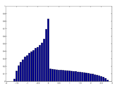
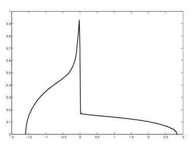
Figure 1: Simulated and limiting spectral density of the random block matrix $G_{n}^{(r)}/\sqrt{n}$ in the case $r=2$, $\gamma_{1}=1$, $\gamma_{2}=1$. In the simulation the eigenvalue distribution of a $5000\times 5000$ matrix was calculated (i.e. m = n/r = 2500).

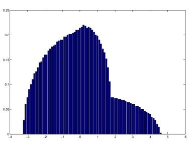
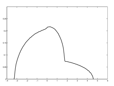
Figure 2: Simulated and limiting spectral density of the random block matrix $G_{n}^{(r)}/\sqrt{n}$ in the case $r=2$, $\gamma_{1}=1$, $\gamma_{2}=5$. In the simulation the eigenvalue distribution of a $5000\times 5000$ matrix was calculated (i.e. m = n/r = 2500).

7 Proofs

7.1 Proof of Proposition 2.1

First we consider the behavior of the roots $z_{k}(x)$ for $x\to\infty$. It is easy to check that in this limit,

$$\left\{\begin{array}[]{ll}z_{k}(x)\to 0,&\qquad k=1,\ldots,r,\\ |z_{k}(x)|\to\infty,&\qquad k=r+1,\ldots,2r,\end{array}\right.$$ (7.1)

see e.g. [10]. In particular we have that $|z_{r}(x)|<|z_{r+1}(x)|$ if $|x|$ is large enough, showing the compactness of $\Gamma_{0}$.

Next we ask the question: for which $x\in\mathbb{C}$ can we have a root $z_{k}=z_{k}(x)$ such that $|z_{k}|=1$? In this case, (2.5) becomes

$$0=f(z_{k},x)=\det(z_{k}A^{*}+B+\overline{z_{k}}A-xI_{r}),$$

so $x$ is an eigenvalue of the Hermitian matrix $z_{k}A^{*}+B+\overline{z_{k}}A$. In particular, it follows that

$$|z_{k}(x)|=1\ \Rightarrow\ x\in\mathbb{R}.$$ (7.2)

Now for $x\to\infty$, (7.1) implies that we have precisely $r$ roots $z_{k}(x)$ with $|z_{k}(x)|<1$. By (7.2) and continuity this must then hold for all $x\in\mathbb{C}\setminus\mathbb{R}$:

$$x\in\mathbb{C}\setminus\mathbb{R}\ \Rightarrow\ \left\{\begin{array}[]{ll}|z_{k}(x)|<1,&\quad k=1,\ldots,r,\\ |z_{k}(x)|>1,&\quad k=r+1,\ldots,2r.\end{array}\right.$$

In particular we see that $|z_{r}(x)|<1<|z_{r+1}(x)|$ for $x\in\mathbb{C}\setminus\mathbb{R}$, implying that $\Gamma_{0}\subset\mathbb{R}$.

Finally, the claim that $\Gamma_{0}\subset\mathbb{R}$ is the disjoint union of at most $r$ intervals follows from [10, 29]. $\hfill\square\\$

7.2 Proof of Lemma 2.2

The proof will use ideas from Durán [13, Proof of Lemma 2.2]. We invoke a general result known as the square-free factorization for multivariate polynomials. In our context it implies that there exists a factorization of the bivariate polynomial $z^{r}f(z,x)$ of the form

$$z^{r}f(z,x)=\prod_{k=1}^{K}g_{k}(z,x)^{m_{k}},$$ (7.3)

for certain $K\in\mathbb{Z}_{>0}$, multiplicities $m_{1},\ldots,m_{K}\in\mathbb{Z}_{>0}$ and non-constant bivariate polynomials $g_{1}(z,x),\ldots,g_{K}(z,x)$, in such a way that

$$g(z,x):=\prod_{k=1}^{K}g_{k}(z,x)$$ (7.4)

is square-free, i.e., for all but finitely many $x\in\mathbb{C}$, the roots $z$ of $g(z,x)=0$ are all distinct, and vice versa with the roles of $x$ and $z$ reversed.

The existence of the square-free factorization of the previous paragraph, can be obtained from a repeated use of Euclid’s algorithm. For example, if $z^{r}f(z,x)=0$ has a multiple root $z=z(x)$ for all $x\in\mathbb{C}$, then we apply Euclid’s algorithm with input polynomials $z^{r}f(z,x)$ and $\frac{\partial}{\partial z}\left(z^{r}f(z,x)\right)$, viewed as polynomials in $z$ with coefficients in $\mathbb{C}[x]$. This gives us the greatest common divisor of these two polynomials and yields a factorization

$$z^{r}f(z,x)=g_{1}(z,x)g_{2}(z,x),$$

for two bivariate polynomials $g_{1},g_{2}$ which depend both nontrivially on $z$. Note that the factorization can be taken fraction free, i.e., with $g_{1},g_{2}$ being polynomials in $x$ rather than rational functions. If one of the factors $g_{1}$ or $g_{2}$ has a multiple root $z=z(x)$ for all $x\in\mathbb{C}$, then we repeat the above procedure. If $g_{1}$ and $g_{2}$ have a common root $z=z(x)$ for all $x\in\mathbb{C}$, then we apply Euclid’s algorithm with input polynomials $g_{1}$ and $g_{2}$, viewed again as polynomials in $z$ with coefficients in $\mathbb{C}[x]$. Repeating this procedure sufficiently many times yields the square-free factorization in the required form.

Note that the factors $g_{k}(z,x)$ in (7.3) all depend non-trivially on both $z$ and $x$. For if $g_{k}(z,x)$ would be a polynomial in $z$ alone (say), then there would exist $z\in\mathbb{C}$ such that $f(z,x)=0$ for all $x\in\mathbb{C}$, which is easily seen to contradict with (2.5).

From the above paragraphs we easily get the symmetry relation

$$m_{1}(z,x)=m_{2}(z,x),$$

for all but finitely many $z,x\in\mathbb{C}$. This proves one part of Lemma 2.2.

It remains to show that $m_{2}(z,x)=d(z,x)$ for all but finitely many $z,x\in\mathbb{C}$. From the definitions, this is equivalent to showing that the matrix $zA^{*}+B+z^{-1}A$ is diagonalizable for all but finitely many $z\in\mathbb{C}$. This is certainly true if $|z|=1$ since then $zA^{*}+B+z^{-1}A$ is Hermitian so in particular diagonalizable. The claim then follows in exactly the same way as in [13, Proof of Lemma 2.2]. $\hfill\square\\$

7.3 Proof of Theorem 2.3

Before going to the proof of Theorem 2.3, let us recall the following result of Dette-Reuther [11]. As mentioned before, this result uses in an essential way the Hermitian structure of (1.2).

Lemma 7.1.

(See [11]:) If all roots of the matrix orthogonal polynomials $P_{n}(x)$ are located in the interval $[-M,M]$, then the inequality

$$|\mathbf{v}^{*}P_{n}(z)P^{-1}_{n+1}(z)A^{-1}_{n+1}\mathbf{v}|\leq\frac{1}{\mathrm{dist}(z,[-M,M])}$$

holds for all complex numbers $z$ and for all column vectors $\mathbf{v}$ with unit Euclidean norm $||\mathbf{v}||=1$.

We will need the following variant of Lemma 7.1:

Corollary 7.2.

In the matrix Nevai class (1.3) we can find $M>0$ as in Lemma 7.1 so that

$$|\mathbf{w}^{*}P_{n}(z)P^{-1}_{n+1}(z)\mathbf{v}|\leq\frac{8||A||}{\mathrm{dist}(z,[-M,M])}$$ (7.5)

for all $n$ sufficiently large, all column vectors $\mathbf{v},\mathbf{w}$ with $||\mathbf{v}||=||\mathbf{w}||=1$ and all complex numbers $z$. Here $||A||$ denotes the operator norm (also known as $2$-norm, or maximal singular value) of the matrix $A$.

Proof.

For fixed $n$ and fixed $z\in\mathbb{C}$, define the sesquilinear form

$$\langle\mathbf{v},\mathbf{w}\rangle_{A}:=\mathbf{w}^{*}P_{n}(z)P^{-1}_{n+1}(z)A^{-1}_{n+1}\mathbf{v},$$

which is linear in its first and antilinear in its second argument. Also define $||\mathbf{v}||_{A}^{2}:=\langle\mathbf{v},\mathbf{v}\rangle_{A}$. (This ‘norm’ is not necessarily positive!) The polar identity asserts that

$$\langle\mathbf{v},\mathbf{w}\rangle_{A}=\frac{1}{4}\left(||\mathbf{v}+\mathbf{w}||_{A}^{2}-||\mathbf{v}-\mathbf{w}||_{A}^{2}+i||\mathbf{v}+i\mathbf{w}||_{A}^{2}-i||\mathbf{v}-i\mathbf{w}||_{A}^{2}\right).$$

Combining this with Lemma 7.1 we get

$$|\mathbf{w}^{*}P_{n}(z)P^{-1}_{n+1}(z)A^{-1}_{n+1}\mathbf{v}|=:|\langle\mathbf{v},\mathbf{w}\rangle_{A}|\leq\frac{4}{\mathrm{dist}(z,[-M,M])}$$

for all pairs of vectors $\mathbf{v},\mathbf{w}$ with $||\mathbf{v}||=||\mathbf{w}||=1$ and for all complex numbers $z$. If we now take $n$ sufficiently large so that $||A_{n+1}||<2||A||$ (recall (1.3)), we get the desired inequality (7.5). ∎

Proof of Theorem 2.3.

We will use a normal family argument. Fix $k\in\{1,\ldots,r\}$ and $z_{0}\in\mathbb{C}\setminus[-M,M]$. By (7.5) we have that $P_{n}(z)P^{-1}_{n+1}(z)\mathbf{v}_{k}(z)$ is uniformly bounded entrywise in a neighborhood of $z=\infty$. By Montel’s theorem we can take a subsequence of indices $(n_{i})_{i=0}^{\infty}$ so that the limit $\lim_{i\to\infty}P_{n_{i}}(z)P^{-1}_{n_{i}+1}(z)\mathbf{v}_{k}(z)$ exists uniformly in this neighborhood. We will prove by induction on $l=0,1,2,\ldots$ that

$$\lim_{i\to\infty}P_{n_{i}}(x)P_{n_{i}+1}^{-1}(x)\mathbf{v}_{k}(x)=z_{k}(x)\mathbf{v}_{k}(x)+O(x^{-l}),\qquad x\to\infty.$$ (7.6)

For $l=0$ (or $l=1$) this follows from (7.5) and the fact that $z_{k}(x)=O(x^{-1})$ as $x\to\infty$.

Now assume that (7.6) is satisfied for a certain value of $l$, and for any sequence $(n_{i})_{i}$ for which the limit exists. Fixing such a sequence $(n_{i})_{i}$, we will prove that (7.6) holds with $l$ replaced by $l+2$. By moving to a subsequence of $(n_{i})_{i}$ if necessary, we may assume without loss of generality that the limiting matrices $\lim_{i\to\infty}P_{n_{i}}(x)P_{n_{i}+1}^{-1}(x)$ and $\lim_{i\to\infty}P_{n_{i}-1}(x)P_{n_{i}}^{-1}(x)$ both exist. The induction hypothesis asserts that (7.6) holds for any sequence $(n_{i})$ for which the limit exists, so in particular

$$\lim_{i\to\infty}P_{n_{i}-1}(x)P_{n_{i}}^{-1}(x)\mathbf{v}_{k}(x)=z_{k}(x)\mathbf{v}_{k}(x)+O(x^{-l}),\qquad x\to\infty.$$ (7.7)

Now let us write the three-term recurrence (1.1) in the form

$$A_{n_{i}}^{*}P_{n_{i}-1}(x)P_{n_{i}}^{-1}(x)+(B_{n_{i}}-xI_{r})+A_{n_{i}+1}P_{n_{i}+1}(x)P_{n_{i}}^{-1}(x)=0.$$

Multiplying on the right with $\mathbf{v}_{k}(x)$, taking the limit $i\to\infty$ and using the facts that $\lim_{n}A_{n}=A$ and $\lim_{n}B_{n}=B$ we get

$$A^{*}\lim_{i\to\infty}\left(P_{n_{i}-1}(x)P_{n_{i}}^{-1}(x)\right)\mathbf{v}_{k}(x)+(B-xI_{r})\mathbf{v}_{k}(x)+A\lim_{i\to\infty}\left(P_{n_{i}+1}(x)P_{n_{i}}^{-1}(x)\right)\mathbf{v}_{k}(x)=0.$$

With the help of (7.7) and (2.2) this implies

$$A\lim_{i\to\infty}\left(P_{n_{i}+1}(x)P_{n_{i}}^{-1}(x)\right)\mathbf{v}_{k}(x)=Az_{k}^{-1}(x)\mathbf{v}_{k}(x)+O(x^{-l}),\qquad x\to\infty.$$

Multiplying this relation on the left with $z_{k}(x)\lim_{n\to\infty}\left(P_{n_{i}}(x)P_{n_{i}+1}^{-1}(x)\right)A^{-1}$ and using (7.5) and the fact that $z_{k}(x)=O(x^{-1})$ for $x\to\infty$, we find

$$\lim_{i\to\infty}P_{n_{i}}(x)P_{n_{i}+1}^{-1}(x)\mathbf{v}_{k}(x)=z_{k}(x)\mathbf{v}_{k}(x)+O(x^{-l-2}),\qquad x\to\infty,$$

showing that the induction hypothesis (7.6) holds with $l$ replaced with $l+2$. This proves the induction step. ∎

7.4 Proof of Theorem 2.5

We write the telescoping product

$$\det P_{n}(x)=\left(\det P_{n}(x)P_{n-1}^{-1}(x)\right)\ldots\left(\det P_{2}(x)P_{1}^{-1}(x)\right)\left(\det P_{1}(x)P_{0}^{-1}(x)\right)\det P_{0}(x).$$

Taking logarithms and dividing by $rn$ we get

$$\frac{1}{rn}\log\det P_{n}(x)=\frac{1}{rn}\left(\left(\sum_{k=1}^{n}\log\det P_{k}(x)P_{k-1}^{-1}(x)\right)+\log\det P_{0}(x)\right).$$

(Here we use the logarithm as a complex multi-valued function.) Taking the limit $n\to\infty$ and using the ratio asymptotics in Corollary 2.4, we obtain

$$-\lim_{n\to\infty}\frac{1}{rn}\log(\det P_{n}(x))=\frac{1}{r}\log(z_{1}(x)\ldots z_{r}(x)),\qquad x\in\mathbb{C}\setminus[-M,M].$$

Now we take the real part of both sides of this equation. Then the left hand side becomes precisely the logarithmic potential of $\mu_{0}$, up to an additive constant $C$. So we obtain (2.13); the constant $C$ can be determined by calculating the asymptotics for $x\to\infty$. $\hfill\square\\$

7.5 Proof of Proposition 2.6

From Proposition 2.1 and its proof we know that both the left and right hand sides of the equation in (2.15) are subsets of the real axis. Now for $x\in\mathbb{R}$ one has the symmetry relation

$$\overline{f(z,x)}:=\overline{\det(A^{*}z+B+Az^{-1}-xI_{r})}=\det(A\bar{z}+B+A^{*}\bar{z}^{-1}-xI_{r})=f(\bar{z}^{-1},x),$$ (7.8)

where the bar denotes the complex conjugation and we used that $\overline{\det M}=\det(M^{*})$ for any square matrix $M$. This implies that for each solution $z=z_{k}(x)$ of the equation $f(z,x)=0$, the complex conjugated inverse $z=\bar{z}_{k}^{-1}(x)$ is a solution as well, with the same multiplicity. So with the ordering (2.4) we have that $|z_{k}(x)|\cdot|z_{2r-k}(x)|=1$ for any $k=1,\ldots,r$. In particular we have that $|z_{r}(x)|=|z_{r+1}(x)|$ if and only if $|z_{r}(x)|=1$. This implies Proposition 2.6. $\hfill\square\\$

7.6 Proof of Proposition 2.7

We use the notations in Section 2.4. We fix $x\in\mathcal{I}\subset\Gamma_{0}$ and define the sets

$$S_{+}(x)=\{z_{k}(x)\mid|z_{k}(y)|<1\textrm{ for all }y\in\Omega\cap\mathbb{C}_{+}\},$$ (7.9)

$$S_{-}(x)=\{z_{k}(x)\mid|z_{k}(y)|<1\textrm{ for all }y\in\Omega\cap\mathbb{C}_{-}\}.$$ (7.10)

So $S_{+}(x)$ (or $S_{-}(x)$) contains all the roots $z_{k}(x)$ for which $|z_{k}(y)|<1$ for $y$ in the upper half plane (or lower half plane respectively) close to $x$.

Let $z_{k}(x)$ be a root of modulus strictly less than $1$. By continuity this root belongs to both sets $S_{+}(x)$ and $S_{-}(x)$, with the same multiplicity, and hence the contributions from the $+$- and $-$-terms in (2.14) corresponding to this root $z_{k}(x)$ cancel out.

Next let $z_{k}(x)$ be a root of modulus $1$. Assume again that $z_{k}(y)=e^{i\theta_{k}(y)}$ with $\theta_{k}(y)$ real and differentiable for $y\in\mathcal{I}\subset\mathbb{R}$. Suppose that $\theta_{k}^{\prime}(x)>0$. Then the Cauchy-Riemann equations applied to $\log z_{k}(y)$ imply that $|z_{k}(y)|<1$ for $y$ in the upper half plane close to $x$, and $|z_{k}(y)|>1$ for $y$ in the lower half plane close to $x$. So $z_{k}(x)$ lies in the set $S_{+}(x)$ in (7.9) but not in $S_{-}(x)$. Similarly if $\theta_{k}^{\prime}(x)<0$ then $z_{k}(x)$ lies in the set $S_{-}(x)$ but not in $S_{+}(x)$. In both cases, the contribution from $z_{k}(x)$ in the right hand side of (2.14) has a positive sign and so we obtain the desired equality (2.16).

Finally, the claim that $\theta^{\prime}(x)\neq 0$ for any $x\in\mathcal{I}\subset\Gamma_{0}$ follows since, if this fails, then general considerations (e.g. in [27, Proof of Theorem 11.1.1(v)]) would imply that $\Gamma_{0}\not\subset\mathbb{R}$, which is a contradiction. $\hfill\square\\$

7.7 Proof of Theorem 3.1

The proof of Theorem 2.3 and 2.5 can be easily extended to prove Theorem 3.1. The difference is that the limits $\lim_{n_{i}\to\infty}$ should be replaced by local limits of the form $\lim_{n_{i}/N\to s}$. The details are straightforward and left to the reader (for similar reasonings see also [3, 7, 11, 20, 22], among others.)

7.8 Proof of Theorem 3.4

The proof of Theorem 3.4 will follow the same scheme as the proof of Theorem 2.3, but it will be more complicated due to the higher periodicity. To deal with the periodicity we will use some ideas from [3]. It is convenient to substitute $z=y^{p}$ and work with the transformed matrix

$$G(y,x) := \operatorname{diag}(1,y,\ldots,y^{p-1})F(y^{p},x)\operatorname{diag}(1,y^{-1},\ldots,y^{-(p-1)})$$ (7.11)

$$= \begin{pmatrix}B^{(0)}-xI_{r}&y^{-1}A^{(1)}&0&0&yA^{(0)*}\\ yA^{(1)*}&B^{(1)}-xI_{r}&y^{-1}A^{(2)}&0&0\\ 0&yA^{(2)*}&\ddots&\ddots&0\\ 0&0&\ddots&\ddots&y^{-1}A^{(p-1)}\\ y^{-1}A^{(0)}&0&0&yA^{(p-1)*}&B^{(p-1)}-xI_{r}\end{pmatrix}_{pr\times pr}.$$ (7.12)

Consistently with the substitution $z=y^{p}$, we put $y_{k}(x)=z_{k}^{1/p}(x)$, $k=1,\ldots,2r$, for an arbitrary but fixed choice of the $p$th root. The ordering (2.4) implies that

$$0<|y_{1}(x)|\leq|y_{2}(x)|\leq\ldots\leq|y_{r}(x)|\leq|y_{r+1}(x)|\leq\ldots\leq|y_{2r}(x)|.$$ (7.13)

Note that each $y=y_{k}(x)$ is a root of the algebraic equation

$$\det G(y,x)\equiv\det F(y^{p},x)=0.$$

From (7.12) it is then easy to check that (see e.g. [10])

$$y_{k}(x)\propto\left\{\begin{array}[]{lll}x^{-1},&k=1,\ldots,r,&x\to\infty,\\ x,&k=r+1,\ldots,2r,&x\to\infty,\end{array}\right.$$ (7.14)

where the $\propto$ symbol means that the ratio of the left and right hand sides is bounded both from below and above in absolute value when $x\to\infty$.

Denote with $\mathbf{w}_{k}(x)$ a normalized null space vector such that

$$G(y_{k}(x),x)\mathbf{w}_{k}(x)=\mathbf{0}.$$ (7.15)

If there are roots $y_{k}(x)$ with higher multiplicities then we pick the vectors $\mathbf{w}_{k}(x)$ as explained in Section 2.2. We again partition $\mathbf{w}_{k}(x)$ in blocks as

$$\mathbf{w}_{k}(x)=\begin{pmatrix}\mathbf{w}_{k,0}(x)\\ \vdots\\ \mathbf{w}_{k,p-1}(x)\end{pmatrix},$$ (7.16)

where each $\mathbf{w}_{k,j}(x)$, $j=0,1,\ldots,p-1$, is a column vector of length $r$. Assuming the normalization $||\mathbf{w}_{k}(x)||=1$ then we have that

$$\lim_{x\to\infty}||\mathbf{w}_{k,j}(x)||=C_{k,j}>0,\qquad j=0,1,\ldots,p-1.$$ (7.17)

This follows from (7.15)–(7.16), (7.14) and by inspecting the dominant terms for $x\to\infty$ in the matrix (7.12).

Theorem 3.4 will be a consequence of the following stronger statement:

$$\left(\lim_{n\to\infty}P_{pn+j}(x)P_{pn+j+1}^{-1}(x)\right)\mathbf{w}_{k,j+1}(x)=y_{k}(x)\mathbf{w}_{k,j}(x),\quad x\to\infty,$$ (7.18)

uniformly for $x$ in compact subsets of $\mathbb{C}\setminus([-M,M]\cup S)$, for all $k\in\{1,\ldots,r\}$ and for all residue classes $j\in\{0,1,\ldots,p-1\}$ modulo $p$. (We identify $\mathbf{w}_{k,p}(x)\equiv\mathbf{w}_{k,0}(x)$.) Indeed, Theorem 3.4 immediately follows by iterating (7.18) $p$ times and using that $y_{k}^{p}(x)=z_{k}(x)$.

The rest of the proof is devoted to establishing (7.18). We will show by induction on $l\geq 0$ that

$$\left(\lim_{i\to\infty}P_{pn_{i}+j}(x)P_{pn_{i}+j+1}^{-1}(x)\right)\mathbf{w}_{k,j+1}(x)=y_{k}(x)\mathbf{w}_{k,j}(x)(1+O(x^{-l})),\quad x\to\infty,$$ (7.19)

for any $k\in\{1,\ldots,r\}$ and $j\in\{0,1,\ldots,p-1\}$, and for any increasing sequence $\left(n_{i}\right)_{i=0}^{\infty}$ for which the limit in the left hand side exists.

Assume that the induction hypothesis (7.19) holds for a certain value of $l\geq 0$. We will show that it also holds for $l+2$. Let $\left(n_{i}\right)_{i=0}^{\infty}$ be an increasing sequence for which the limit in the left hand side of (7.19) exists. We can assume without loss of generality that $j=p-1$; a similar argument will work for the other values of $j\in\{0,1,\ldots,p-1\}$. Now from the three-term recursion we obtain

$$\begin{pmatrix}A_{pn_{i}}^{*}&B_{pn_{i}}-xI_{r}&A_{pn_{i}+1}\\ &A_{pn_{i}+1}^{*}&\ddots&\ddots\\ &&\ddots&\ddots&A_{pn_{i}+p-1}\\ &&&A_{pn_{i}+p-1}^{*}&B_{pn_{i}+p-1}-xI_{r}&A_{pn_{i}+p}\end{pmatrix}\begin{pmatrix}P_{pn_{i}-1}(x)\\ P_{pn_{i}}(x)\\ \vdots\\ P_{pn_{i}+p-1}(x)\\ P_{pn_{i}+p}(x)\end{pmatrix}=0.$$ (7.20)

Applying a diagonal multiplication with appropriate powers of $y:=y_{k}(x)$ we get

$$\begin{pmatrix}yA_{pn_{i}}^{*}&B_{pn_{i}}-xI_{r}&y^{-1}A_{pn_{i}+1}\\ &yA_{pn_{i}+1}^{*}&\ddots&\ddots\\ &&\ddots&\ddots&y^{-1}A_{pn_{i}+p-1}\\ &&&yA_{pn_{i}+p-1}^{*}&B_{pn_{i}+p-1}-xI_{r}&y^{-1}A_{pn_{i}+p}\end{pmatrix}\begin{pmatrix}y^{-p}P_{pn_{i}-1}(x)\\ y^{-(p-1)}P_{pn_{i}}(x)\\ \vdots\\ y^{-1}P_{pn_{i}+p-2}(x)\\ P_{pn_{i}+p-1}(x)\\ yP_{pn_{i}+p}(x)\end{pmatrix}=0.$$ (7.21)

Let us focus on the rightmost matrix in the left hand side of (7.21). Multiplying on the right with $P_{pn_{i}+p-1}^{-1}(x)\mathbf{w}_{k,p-1}(x)$ it becomes

$$\begin{pmatrix}y^{-p}P_{pn_{i}-1}P_{pn_{i}+p-1}^{-1}\mathbf{w}_{k,p-1}\\ \vdots\\ y^{-1}P_{pn_{i}+p-2}P_{pn_{i}+p-1}^{-1}\mathbf{w}_{k,p-1}\\ \mathbf{w}_{k,p-1}\\ yP_{pn_{i}+p}P_{pn_{i}+p-1}^{-1}\mathbf{w}_{k,p-1}\end{pmatrix}.$$ (7.22)

(Here we skip the $x$-dependence for notational simplicity.) By moving to a subsequence of $(n_{i})_{i=0}^{\infty}$ if necessary and using compactness, we may assume that each block of (7.22) has a limit for $i\to\infty$. Repeated application of the induction hypothesis (7.19) then implies that the limit of (7.22) for $i\to\infty$ behaves as

$$\begin{pmatrix}\mathbf{w}_{k,p-1}(1+O(x^{-l}))\\ \mathbf{w}_{k,0}(1+O(x^{-l}))\\ \vdots\\ \mathbf{w}_{k,p-2}(1+O(x^{-l}))\\ \mathbf{w}_{k,p-1}\\ \varphi(x)\end{pmatrix},$$

for $x\to\infty$, where

$$\varphi(x):=\left(\lim_{i\to\infty}P_{pn_{i}+p}(x)P_{pn_{i}+p-1}^{-1}(x)\right)y_{k}(x)\mathbf{w}_{k,p-1}(x).$$ (7.23)

Multiplying (7.21) on the right with $P_{pn_{i}+p-1}^{-1}(x)\mathbf{w}_{k,p-1}(x)$ and taking the limit $i\to\infty$, we get from the above observations that

$$\begin{pmatrix}yA^{(0)*}&B^{(0)}-xI_{r}&y^{-1}A^{(1)}\\ &yA^{(1)*}&\ddots&\ddots\\ &&\ddots&\ddots&y^{-1}A^{(p-1)}\\ &&&yA^{(p-1)*}&B^{(p-1)}-xI_{r}&y^{-1}A^{(0)}\end{pmatrix}\begin{pmatrix}\mathbf{w}_{k,p-1}\\ \mathbf{w}_{k,0}\\ \vdots\\ \mathbf{w}_{k,p-2}\\ \mathbf{w}_{k,p-1}\\ \varphi(x)\end{pmatrix}=\begin{pmatrix}O(x^{-l+1})\\ \vdots\\ O(x^{-l+1})\\ O(x^{-l-1})\end{pmatrix},$$ (7.24)

for $x\to\infty$, where we used that $y\equiv y_{k}(x)\propto x^{-1}$ for $x\to\infty$. Taking the last block row of this equation yields

$$y_{k}(x)A^{(p-1)*}\mathbf{w}_{k,p-2}+(B^{(p-1)}-xI_{r})\mathbf{w}_{k,p-1}+y_{k}^{-1}(x)A^{(0)}\varphi(x)=O(x^{-l-1}).$$ (7.25)

On the other hand, by (7.15), (7.16) and (7.12) (evaluated for the last block row) we have that

$$y_{k}^{-1}(x)A^{(0)}\mathbf{w}_{k,0}+y_{k}(x)A^{(p-1)*}\mathbf{w}_{k,p-2}+(B^{(p-1)}-xI_{r})\mathbf{w}_{k,p-1}=0.$$

Subtracting this from (7.25) we get

$$A^{(0)}\left(\lim_{i\to\infty}P_{pn_{i}+p}(x)P_{pn_{i}+p-1}^{-1}(x)\right)\mathbf{w}_{k,p-1}(x)-y_{k}^{-1}(x)A^{(0)}\mathbf{w}_{k,0}(x)=O(x^{-l-1}),$$

on account of (7.23). The factor $A^{(0)}$ can be skipped from this equation. Then multiplying on the left with $y_{k}(x)\times\left(\lim_{i\to\infty}P_{pn_{i}+p-1}(x)P_{pn_{i}+p}^{-1}(x)\right)$ we get

$$\left(\lim_{i\to\infty}P_{pn_{i}+p-1}(x)P_{pn_{i}+p}^{-1}(x)\right)\mathbf{w}_{k,0}(x)-y_{k}(x)\mathbf{w}_{k,p-1}(x)=O(x^{-l-3}),$$

or equivalently

$$\left(\lim_{i\to\infty}P_{pn_{i}+p-1}(x)P_{pn_{i}+p}^{-1}(x)\right)\mathbf{w}_{k,0}(x)=y_{k}(x)\mathbf{w}_{k,p-1}(x)(1+O(x^{-l-2})).$$

We conclude that (7.19) holds with $l$ replaced by $l+2$. This proves the induction step. $\hfill\square\\$

7.9 Proof of Proposition 4.2

Throughout the proof we will use the notations of Section 4. Recall that the Hermitian symmetry $A=A^{*}$ implies the roots $z_{k}(x)$ to appear in pairs $\{z_{k}(x),z_{k}(x)^{-1}\}$. Both $z_{k}(x)$ and $z_{k}(x)^{-1}$ correspond to the same value of $w_{k}(x)=z_{k}(x)+z_{k}(x)^{-1}$ in (4.9) and therefore to the same null space vector $\mathbf{v}_{k}(x)$.

Now let $x\in\mathbb{R}$. For any $w_{k}(x)=2\cos\theta_{k}(x)\in(-2,2)$, with $\theta\in(0,\pi)$, $k=1,\ldots,r$, we have a pair of roots $z_{k_{1}}(x)=e^{i\theta_{k}(x)}$ and $z_{k_{2}}(x)=e^{-i\theta_{k}(x)}$, with $\{k_{1},k_{2}\}=\{k,2r-k\}$. Suppose that $w_{k}^{\prime}(x)>0$. Then the Cauchy-Riemann equations show that $z_{k_{1}}(x)$ lies in the set $S_{-}(x)$ in (7.10) but not in $S_{+}(x)$, and vice versa for the root $z_{k_{2}}(x)$. The reverse situation occurs if $w_{k}^{\prime}(x)<0$.

Fix $x\in\mathbb{R}$ and assume the labeling of roots is such that

$$\max\{|z_{1}(x)|,\ldots,|z_{K}(x)|\}<1,\qquad|z_{K+1}(x)|=\ldots=|z_{r}(x)|=1,$$

with $K\in\{0,\ldots,r\}$. Taking into account the above observations, we find from (4.2) that

$$\lim_{\epsilon\to 0+}F_{W}(x+\epsilon i)$$

$$= V(x)\left(\lim_{\epsilon\to 0+}D(x+\epsilon i)\right)V^{-1}(x)A^{-1}$$

$$= V(x)\operatorname{diag}(z_{1}(x),\ldots,z_{K}(x),e^{-i\theta_{K+1}(x)\mathrm{sign}\,w_{K+1}^{\prime}(x)},\ldots,e^{-i\theta_{r}(x)\mathrm{sign}\,w_{r}^{\prime}(x)})V^{-1}(x)A^{-1}.$$

Similarly

$$\lim_{\epsilon\to 0+}F_{W}(x-\epsilon i)$$

$$= V(x)\left(\lim_{\epsilon\to 0+}D(x-\epsilon i)\right)V^{-1}(x)A^{-1}$$

$$= V(x)\operatorname{diag}(z_{1}(x),\ldots,z_{K}(x),e^{i\theta_{K+1}(x)\mathrm{sign}\,w_{K+1}^{\prime}(x)},\ldots,e^{i\theta_{r}(x)\mathrm{sign}\,w_{r}^{\prime}(x)})V^{-1}(x)A^{-1}.$$

Using the Stieltjes inversion principle

$$\frac{\mathrm{d}W(x)}{\mathrm{d}x}=\frac{1}{2\pi i}\lim_{\epsilon\to 0+}\left(F_{W}(x-\epsilon i)-F_{W}(x+\epsilon i)\right),$$

the desired formula for $\mathrm{d}W/\mathrm{d}x$ now follows from a straightforward calculation. The formula for $\mathrm{d}X/\mathrm{d}x$ similarly follows from (4.4), taking into account the simplifications due to $A=A^{*}$. $\hfill\square\\$

Acknowledgements The work of the authors is supported by the SFB TR12 ”Symmetries and Universality in Mesoscopic Systems”, Teilprojekt C2. The first author is a Postdoctoral Fellow of the Fund for Scientific Research - Flanders (Belgium). His work is supported in part by the Belgian Interuniversity Attraction Pole P06/02. The authors would also like to thank Martina Stein, who typed parts of this manuscript with considerable technical expertise.

References

- [1] A.I. Aptekarev, G. López Lagomasino, and I.A. Rocha, Ratio asymptotic of Hermite-Padé orthogonal polynomials for Nikishin systems, Math. Sb. 196 (2005), 1089–1107.
- [2] A. Aptekarev and E. Nikishin, The scattering problem for a discrete Sturm-Liouville operator, Mat. Sb. 121 (1983), 327 -358.
- [3] M. Bender, S. Delvaux and A.B.J. Kuijlaars, Multiple Meixner-Pollaczek polynomials and the six-vertex model, J. Approx. Theory 163 (2011), 1606–1637.
- [4] J. Borrego, M. Castro and A. Durán, Orthogonal matrix polynomials satisfying differential equations with recurrence coefficients having non-scalar limits, Integral Transforms Spec. Funct. 23 (2012), 685–700.
- [5] A. Böttcher and B. Silbermann, Introduction to Large Truncated Toeplitz Matrices, Universitext, Springer-Verlag, New York, 1998.
- [6] M.J. Cantero, F.A. Grünbaum, L. Moral and L. Velazquez, Matrix valued Szegő polynomials and quantum walks, Comm. Pure Appl. Math. 63 (2010), 464–507.
- [7] E. Coussement, J. Coussement and W. Van Assche, Asymptotic zero distribution for a class of multiple orthogonal polynomials, Trans. Amer. Math. Soc. 360 (2008), 5571–5588.
- [8] D. Damanik, A. Pushnitski and B. Simon, The analytic theory of matrix orthogonal polynomials, Surv. Approx. Theory 4 (2008), 1–85.
- [9] D. Damanik, R. Killip and B. Simon, Perturbations of orthogonal polynomials with periodic recursion coefficients, Ann. of Math. 171 (2010), 1931–2010.
- [10] S. Delvaux, Equilibrium problem for the eigenvalues of banded block Toeplitz matrices, Math. Nachr. 285 (2012), 1935 1962.
- [11] H. Dette and B. Reuther, Random Block Matrices and Matrix Orthogonal Polynomials, J. Theor. Probab. (2008), DOI 10.1007/s10959-008-0189-z.
- [12] I. Dumitriu and A. Edelman, Matrix models for beta ensembles, J. Math. Phys. 43 (2002), 5830-5847.
- [13] A. Durán, Ratio asymptotics for Orthogonal Matrix Polynomials, J. Approx. Theory 100 (1999), 304–344.
- [14] A. Durán and P. López-Rodriguez, Orthogonal matrix polynomials: Zeros and Blumenthal’s theorem, J. Approx. Theory 84 (1996), 96–118.
- [15] A. Durán, P. López-Rodriguez and E. Saff, Zero asymptotic behaviour for orthogonal matrix polynomials, J. Anal. Math. 78 (1999), 37–60.
- [16] F.J. Dyson, The threefold way. Algebraic structure of symmetry groups and ensembles in quantum mechanics. J. Math. Phys. 3 (1962), 1199-1215.
- [17] F.A. Grünbaum, M.D. de la Iglesia and A. Martínez-Finkelshtein, Properties of matrix orthogonal polynomials via their Riemann-Hilbert characterization, SIGMA 7 (2011), 098.
- [18] R. Kozhan, Equivalence classes of block Jacobi matrices, Proc. Amer. Math. Soc. 139 (2011), 799–805.
- [19] M.G. Krein, Infinite J-matrices and a matrix moment problem, Dokl. Akad. Nauk SSSR 69 (1949), 125 -128 (in Russian).
- [20] A.B.J. Kuijlaars and P. Román, Recurrence relations and vector equilibrium problems arising from a model of non-intersecting squared Bessel paths, J. Approx. Theory 162 (2010), 2048–2077.
- [21] A.B.J. Kuijlaars and S. Serra-Capizzano, Asymptotic zero distribution of orthogonal polynomials with discontinuously varying recurrence coefficients, J. Approx. Theory 113 (2001), 142-155.
- [22] A.B.J. Kuijlaars and W. Van Assche, The asymptotic zero distribution of orthogonal polynomials with varying recurrence coefficients, J. Approx. Theory 99 (1999), 167–197.
- [23] M.L. Mehta, Random Matrices (1967), Academic Press, New York.
- [24] A. Maté and P. Nevai, A generalization of Poincaré’s theorem for recurrence equations, J. Approx. Theory 63 (1990), 92–97.
- [25] E.A. Rakhmanov, On the asymptotics of the ratio of orthogonal polynomials, Math. USSR Sbornik 32 (1977), 199–213.
- [26] E.B. Saff and V. Totik, Logarithmic Potentials with External Field, Springer-Verlag, Berlin, 1997.
- [27] B. Simon, Orthogonal Polynomials on the Unit Circle. Part 2: Spectral Theory, Amer. Math. Soc. Coll. Publ. Vol. 54, Amer. Math. Soc. Providence, R.I. 2005.
- [28] B. Simon, Szegő’s Theorem and its Descendants, Princeton university press, 2010.
- [29] H. Widom, Asymptotic behavior of block Toeplitz matrices and determinants, Advances in Math. 13 (1974), 284–322.
- [30] H.O. Yakhlef and F. Marcellán, Orthogonal matrix polynomials, connection between recurrences on the unit circle and on a finite interval, in: Approximation, Optimization and Mathematical Economics (Pointe-a-Pitre, 1999), pp. 369 -382, Physica, Heidelberg, 2001.
- [31] M. Zygmunt, Matrix Chebyshev polynomials and continued fractions, Lin. Alg. Appl. 340 (2002), 150–168.