Abstract

Inspired by soliton models, we propose a description of static particles in terms of Riemannian 4-manifolds with self-dual Weyl tensor. For electrically charged particles, the 4-manifolds are non-compact and asymptotically fibred by circles over physical 3-space. This is akin to the Kaluza-Klein description of electromagnetism, except that we exchange the roles of magnetic and electric fields, and only assume the bundle structure asymptotically, away from the core of the particle in question. We identify the Chern class of the circle bundle at infinity with minus the electric charge and the signature of the 4-manifold with the baryon number. Electrically neutral particles are described by compact 4-manifolds. We illustrate our approach by studying the Taub-NUT manifold as a model for the electron, the Atiyah-Hitchin manifold as a model for the proton, $\mathbb{CP}^{2}$ with the Fubini-Study metric as a model for the neutron, and $S^{4}$ with its standard metric as a model for the neutrino.

1 Introduction

Geometry and the quantum mechanics of particles have an uneasy relationship which is why general relativity is hard to incorporate into quantum field theory. String theory is an ambitious and remarkable attempt at unification with many successes but the final theory has proved mysterious and elusive.

Einstein and Bohr fought a long battle on this front and Bohr was generally deemed to have won, with the Copenhagen interpretation of quantum mechanics accepted. But Einstein’s belief in the role of geometry made a partial come-back with the adoption of gauge theories as models of particle physics.

A more modest and limited role for geometry in nuclear physics was proposed by Skyrme [1] with the solitonic model of baryons, i.e. proton, neutron and nuclei, now known as Skyrmions. These have been shown to be approximate models of the physical baryons occurring in gauge theories of quarks and gluons, and have been extensively studied [2] with considerable success.

In this paper we explore a geometric model of particles which is inspired by Skyrme’s idea but with potential applications to both baryonic and leptonic particle physics. Our model differs from the Skyrme model in that it uses Riemannian geometry rather than field theory, and so it is closer in spirit to Einstein’s ideas. Another key difference is that we absorb the Kaluza-Klein idea of an extra circle dimension to incorporate electromagnetism. However, we exchange the roles of electricity and magnetism relative to the standard Kaluza-Klein approach, so that the extra circle dimension is magnetic rather than electric, and it is the electric charge that is topologically quantised by the famous Dirac argument. We will also, initially, ignore time and dynamics, focusing on purely static models.

Our geometric models will therefore be 4-dimensional Riemannian manifolds. We require the manifolds to be oriented and complete but not usually compact: we use non-compact manifolds to model electrically charged particles, and compact manifolds for neutral particles. Both baryon number and electric charge will be encoded in the topology, with baryon number (at least provisionally) identified with the signature of the 4-manifold and electric charge with minus the Chern class of an asymptotic fibration by circles. In particular, the number of protons and the number of neutrons will therefore be determined topologically.

The manifolds will also have an ‘asymptotic’ structure which captures their relation to physical 3-space. The non-compact manifolds we consider have an asymptotic region which is fibred over physical 3-space, so no additional structure is required. For the compact (neutral) models, however, we fix a distinguished embedded surface $X$ where the 4-manifold $M$ intersects physical 3-space. We also call $M\setminus X$ the inside of $M$.

For single particles, the symmetry group of rotations should fix all of the above data. It should act isometrically on the 4-manifold and preserve the asymptotic structure. In the non-compact cases this means that it should be a bundle map in the asymptotic region, covering the usual $SO(3)$-action on physical 3-space. In the compact cases it should preserve the distinguished surface $X$. In order to capture the fermionic nature of the particles considered in this paper we also require spin structures on the non-compact manifolds and on the inside (in the sense defined above) of compact manifolds. Moreover, the lift of the rotation group action to the spin bundle (over the entire manifold in the non-compact case and over the inside in the compact case) should necessarily be an $SU(2)$-action, and this is what we mean by saying that our models are fermionic.

A key restriction on (the conformal classes of) our manifolds is that they are self-dual. Recall that the Riemann curvature is made up of the Ricci tensor plus the Weyl tensor $W$, which is conformally invariant. In dimension 4, $W$ is the sum of self-dual and anti-self-dual parts

$$W=W^{+}\oplus W^{-}\,.$$ (1.1)

A 4-manifold $M$ is said to be self-dual if $W^{-}=0$. These manifolds are precisely those which have twistor spaces in the sense of Penrose [3]. The latter are 3-dimensional complex manifolds $Z$ with a real $S^{2}$-fibration over $M$. The complex structure of $Z$ (together with a real involution which is the antipodal map on each $S^{2}$) encodes the entire conformal structure of $M$. Even the Einstein metric can be captured by complex data on $Z$.

A simply-connected self-dual 4-manifold, for which the Ricci tensor is also zero, is a hyperkähler manifold, whose structure group reduces to $SU(2)$. It is a complex Kähler manifold for an $S^{2}$-family of complex structures, but for any of these complex structures, and for the complex orientation, it would be anti-self-dual. Since we want self-dual manifolds we choose the opposite orientation.

While some of our particles, including the proton, will be modelled by hyperkähler manifolds, we do not want to be so restrictive. Instead we will only require our 4-manifold models of particles to be self-dual and Einstein, so there can be a non-zero scalar curvature. Our model for the neutron is of this type, distinguishing it from the proton. The neutron will of course also have electric charge zero.

We should point out that reversing the orientation of a 4-manifold turns a self-dual manifold into an anti-self-dual one. This should be interpreted as giving the geometric model of an anti-particle. The existence of anti-particles follows from $CPT$ invariance, and our models are compatible with this.

Self-dual 4-manifolds are, in many ways, the 4-dimensional analogue of Riemann surfaces, with $H_{2}$ replacing $H_{1}$ in homology. In particular there are theorems [4] which assert that such manifolds admit connected sums although, unlike in the case of Riemann surfaces, there are restrictions on when this is possible. Such connected sums model composite objects, like nuclei. Although we focus at present on static particles we do envisage a deformation theory, using the moduli space of self-dual manifolds, which could underlie particle interactions.

Fortunately a lot is now known about self-dual 4-manifolds with many metrics explicitly calculated. This makes it possible to put forward some definite models for the proton and neutron. Even though our ideas are inspired by Skyrme’s theory of baryons, it turns out that geometric models of leptons, i.e. the electron and (electron-)neutrino, are even simpler, and we shall describe them too in the class of self-dual manifolds. Thus, somewhat surprisingly, our framework of self-dual manifolds allows us to describe baryons and leptons in a unified fashion.

The language and spirit of our model for particles is close to that of general relativity and suggests the possibility of a unification with gravity, but we do not address this issue here. In particular, we do not specify an action functional. Instead, we focus on how our model describes general features of particles such as their various quantum numbers. We are aware that a description of elementary particles as 4-dimensional Riemannian manifolds is radically different from established treatments in terms of quantum field theory. What we aim to show in this paper is that such a geometric approach is possible, and that it has some surprising and attractive features, such as the possibility of describing the electron and the proton in one framework. While we do propose definite identifications of certain 4-manifolds with specific particles in Sects. 3-5 of this paper, these should be seen as illustrations of the geometric approach, not necessarily as final proposals.

The paper is organised as follows. In Sect. 2 we outline the genesis of our geometric models of particles, starting with the Skyrme model of baryons. Electrically charged particles are necessarily described by non-compact 4-manifolds in our approach, and in Sect. 3 we explain how to model the electron and proton in terms of the Taub-NUT and Atiyah-Hitchin manifolds, respectively. Neutral particles are described by compact 4-manifolds, and this is discussed in Sects. 4-5. We propose $\mathbb{CP}^{2}$ as a model for the neutron and $S^{4}$ as a model for the neutrino. These are the simplest choices, but we also discuss some more sophisticated versions. In Sect. 6 we describe how our particle models glue into empty space, and how the particles may interact with each other. Sect. 7 contains an outline of how our geometric models capture the spinorial nature of the particles they describe. In Sect. 8 we give the dictionary which translates topological properties of 4-manifolds into the electric charge and baryon number of particles, and discuss in some detail how these charges are related to fields and densities used in conventional Lagrangian models of particle physics. Sect. 9 contains our conclusion and some ideas for follow-up work. Conventions and calculations are collected in appendices A,B and C.

2 From Skyrmions to 4-manifolds

We begin by spelling out in detail how the Skyrme model suggests our 4-manifold model. The Skyrme model is based on a group-valued field from $\mathbb{R}^{3}$,

$$U:\mathbb{R}^{3}\rightarrow G\,,$$ (2.1)

where the Lie group $G$ is usually taken to be $SU(2)$, and $U({\mbox{\boldmath$x$}})\rightarrow 1$ as $|{\mbox{\boldmath$x$}}|\rightarrow\infty$. The degree of $U$ as a map $S^{3}\rightarrow SU(2)$ is identified with baryon number. The minima of the Skyrme energy, for each baryon number, are called Skyrmions.

Skyrmions are free to rotate, both in physical space and through conjugation by elements of $SU(2)$. Quantising this motion gives the Skyrmions spin and electric charge. The proton and neutron, for example, are distinct quantum states of the essentially unique Skyrmion of degree 1.

In [5] it was shown how to generate such Skyrme fields naturally by starting with an $SU(2)$ Yang-Mills gauge field on $\mathbb{R}^{4}$ and calculating the holonomy along the 4th direction. Suitable asymptotic behaviour on $\mathbb{R}^{4}$ guarantees a well-defined map $U$. Although this construction does not preserve the respective energy functionals it does provide a good way of using instantons on $\mathbb{R}^{4}$ (i.e. self-dual gauge fields) to construct approximate minima of the Skyrme energy. It also identifies instanton number with the Skyrme degree. See also the recent papers [6, 7] where the difference between the Yang-Mills and Skyrme energy functionals is interpreted as due to an infinite tower of mesons.

Since the Yang-Mills energy functional in dimension 4 is conformally invariant we could replace the decomposition

$$\mathbb{R}^{4}=\mathbb{R}^{3}\times\mathbb{R}^{1}$$ (2.2)

by

$$S^{4}\setminus S^{2}=H^{3}\times S^{1}\,,$$ (2.3)

where $H^{3}$ is hyperbolic 3-space. In fact we can vary the curvature of $H^{3}$ provided we rescale the circle $S^{1}$ the opposite way, so that large circles correspond to almost flat $H^{3}$. We can now fix a gauge field on $S^{4}\setminus S^{2}$ and take the holonomy round the circles. There are some technicalities (due to base-points) which we shall ignore but basically we expect to end up with a Skyrmion on $H^{3}$, an idea which has been explored in [8].

Now replace $H^{3}\times S^{1}$ by any Riemannian 4-manifold $M$ which is asymptotically fibred by circles over $\mathbb{R}^{3}$. This is the kind of Kaluza-Klein 4-manifold we are going to consider. An $SU(2)$ gauge field on $M$ would then give a Skyrme field on ‘the quotient of $M$ by $S^{1}$’. Since we do not want to assume there is a global circle fibration, this Skyrme field will only be defined asymptotically outside some ‘core’. But an oriented 4-manifold has two natural $SU(2)$ bundles over it, the two spin bundles $S^{+}$ and $S^{-}$ (assuming $M$ is a spin-manifold, i.e. $w_{2}(M)=0$). Picking one of these, say $S^{+}$, we then get from the connection on $S^{+}$ a natural construction of an asymptotic Skyrme field on $\mathbb{R}^{3}$.

This is roughly the genesis of our idea to model particles by 4-manifolds, but the topology of these asymptotic Skyrme fields does not quite fit, and would not give integer baryon numbers as defined in our model. The reason lies in a fundamental difference between the topology of gauge bundles which can have arbitrary instanton number (or second Chern class) and the topology of tangent bundles, where there are divisibility theorems. For example the first Pontrjagin class of a 4-manifold (compact and oriented) is divisible by 3 and then gives the signature. An example is $\mathbb{CP}^{2}$ which has signature 1 and Pontrjagin class 3 (times the generator of $H^{4}(\mathbb{CP}^{2})$).

In the Skyrme model the basic idea is that baryon number is identified with the degree of the map $U$ in (2.1), or equivalently with the instanton number (or second Chern class) of the $SU(2)$ bundle over $\mathbb{R}^{4}$. This differs from the 4-manifold model we want to explore, where baryon number is identified with the signature of the 4-manifold. The signature is additive under taking connected sums of 4-manifolds [9], and this captures the additivity of baryon number for composites of particles, for example, fusion of nuclei. The integrality of the signature is linked to it being an index of an elliptic operator. This means we are in the realm of K-theory rather than cohomology. A consequence of this change of viewpoint is that the geometry of the 4-manifold model is important for us, but we will not try to define a global 3-dimensional Skyrme field $U$.

Recall that in the Skyrme model, baryon number is cohomological and electric charge arises at the quantum level. For our 4-manifold model, electric charge is cohomological, arising, as already explained, from the first Chern class of the asymptotic $S^{1}$-fibration, while baryon number as just indicated should be seen as an index.

To sum up our discussion, we see that our model goes beyond the Skyrme model in aiming to understand topologically both the basic integer physical invariants, baryon number and electric charge. The two models are different, but possibly dual in a suitable sense. We hope to explore this in detail at a later stage.

3 Models for the electron and proton

Models for the basic particles should exhibit a high degree of symmetry and we expect the rotation group $SO(3)$ of $\mathbb{R}^{3}$, or its double cover $SU(2)$, to act as isometries. For electrically charged particles, we take our geometric models to be non-compact hyperkähler manifolds. We also assume that the volume grows with the third power of the radius, to allow for an interpretation of the asymptotic region in terms of physical 3-space. As recently shown in [10], this forces the hyperkähler manifold to be ALF. We are therefore looking for rotationally symmetric and complete ALF hyperkähler manifolds. There are just two possibilities:

1. The Taub-NUT manifold [11, 12] depending on a positive parameter $m$ (interpreted as mass in the gravitational context). For brevity we denote it by TN.

2. The Atiyah-Hitchin manifold, the (simply-connected double cover of the) moduli space of centred $SU(2)$-monopoles of charge two [13]. For brevity we denote it by AH.

Note that we could also single out TN and AH among non-compact, complete and rotationally symmetric hyperkähler manifolds by demanding that the $SU(2)$- (or $SO(3)$-) action rotates the complex structures, see our discussion following (B.12). This turns out to play a role in recovering the usual rotation action on physical 3-space in the asymptotic region of our geometric models, as discussed in Sect. 7.

Both TN and AH can be parametrised in terms of a radial coordinate $r$ and angular coordinates on $SU(2)$ (for TN) or $SO(3)/\mathbb{Z}_{2}$ (for AH). Details are given in Appendix B. In terms of the left-invariant 1-forms defined in (B.1), the metrics of both TN and AH can be written as

$$ds^{2}=f(r)^{2}dr^{2}+a(r)^{2}\eta_{1}^{2}+b(r)^{2}\eta_{2}^{2}+c(r)^{2}\eta_{3}^{2}\,,$$ (3.1)

with the functions $f,a,b,c$ satisfying the self-duality equations

$$\frac{2bc}{f}\frac{da}{dr}=(b-c)^{2}-a^{2}\,,\qquad\mbox{+ cyclic}\,,$$ (3.2)

where + cyclic means we add the two further equations obtained by cyclic permutation of $a,b,c$. We adopt the convention

$$f(r)=-\frac{b(r)}{r}\,,$$ (3.3)

where (for reasons that will emerge later) the radial coordinate $r$ has the range $[0,\infty)$ for TN and $[\pi,\infty)$ for AH. The self-duality equations (3.2) become

$$\frac{da}{dr} =\frac{1}{2rc}(a^{2}-(b-c)^{2})\,,$$

$$\frac{db}{dr} =\frac{b}{2rca}(b^{2}-(c-a)^{2})\,,$$

$$\frac{dc}{dr} =\frac{1}{2ra}(c^{2}-(a-b)^{2})\,.$$ (3.4)

This system has solutions in terms of elementary functions

$$a(r)=b(r)=r\sqrt{\epsilon+\frac{m}{r}}\qquad\mbox{and}\qquad c=\frac{m}{\sqrt{\epsilon+\frac{m}{r}}}\,,$$ (3.5)

with parameters $\epsilon,m>0$, associated to the TN manifold. The topology is that of $\mathbb{R}^{4}$, and as $\epsilon\rightarrow 0$ the metric tends to the flat metric. For $\epsilon>0$ the manifold is asymptotic to an $S^{1}$ fibre-bundle over $\mathbb{R}^{3}$ with the length of the circle being $4\pi m/\sqrt{\epsilon}$. There is a $U(1)$ symmetry acting along the fibres, with just one fixed point at the origin, $r=0$. The whole isometry group is $U(2)$. As $\epsilon\rightarrow 0$ the $U(1)$-action becomes the scalar action on $\mathbb{C}^{2}$. The complex orientation of $\mathbb{C}^{2}$ determines the orientation of TN as a self-dual manifold; this is opposite to the orientation given by any of the complex structures in the hyperkähler family, see Appendix A.6 for a discussion. At infinity, the $U(1)$-action gives the standard Hopf line bundle over $\mathbb{CP}^{1}$ with Chern class $+1$; details are given in Appendix A.

The TN metric with coefficient functions (3.5) has the following behaviour under scaling by non-vanishing real numbers $\alpha,\beta$:

$$r\rightarrow\frac{\beta}{\alpha}\,r\,,\quad m\rightarrow\alpha\beta m\,,\quad\epsilon\rightarrow\alpha^{2}\epsilon\,,\qquad\text{then}\quad ds^{2}\rightarrow\beta^{2}ds^{2}\,.$$ (3.6)

We use rescaling by $\alpha$ to set $\epsilon=1$, and rescaling by $\beta$ to set $m=2$ from now on. This amounts to picking a unit of length for the radial coordinate $r$ and to fixing an overall scale for the metric. Our choice is motivated by the asymptotic form of the AH metric, to be discussed below. Note that, with this choice, the length of the asymptotic circle, in the length units chosen, is $8\pi$.

The solution which gives rise to AH has the asymptotic form, for large $r$,

$$a(r)\sim b(r)\sim r\sqrt{1-\frac{2}{r}}\qquad\mbox{and}\qquad c(r)\sim-\frac{2}{\sqrt{1-\frac{2}{r}}}\,.$$ (3.7)

These asymptotic expressions, a TN metric with $\epsilon=1,m=-2$, also satisfy (3). However $a(r)$ is not actually equal to $b(r)$, and $r$ only extends down to $\pi$. For $r$ near $\pi$, (3.7) is a poor approximation. Instead, one finds the leading terms

$$a(r)\sim 2(r-\pi)\,,\quad b(r)\sim\pi+\frac{1}{2}(r-\pi)\,,\quad c(r)\sim-\pi+\frac{1}{2}(r-\pi)\,,$$ (3.8)

which we will need later in this paper.

The manifold AH is the complement of $\mathbb{RP}^{2}$ (the real projective plane) embedded in $\mathbb{CP}^{2}$, and the complex orientation of $\mathbb{CP}^{2}$ determines the orientation of AH as a self-dual manifold. As for TN this is opposite to the orientation given by any of the complex structures in the hyperkähler family; see our discussion in Appendix A.6. AH has an $SO(3)$ symmetry with just one 2-dimensional orbit at $r=\pi$, which is a minimal 2-sphere. We refer to this minimal 2-sphere, which is the totally imaginary conic in $\mathbb{CP}^{2}$ and determined by $z_{1}^{2}+z_{2}^{2}+z^{2}_{3}=0$ in the homogeneous coordinates introduced in Sect. 4.1, as the core. Asymptotically, the manifold is fibred by circles. As further discussed below, neither the circles nor the base space of this asymptotic fibration are oriented because of a $\mathbb{Z}_{2}$-identification, given explicitly in (B.7).

The manifold TN is usually interpreted as the geometry of a Dirac monopole at the origin [14, 15, 16]. For us, with electric and magnetic charges reversed, it has to be interpreted as an electrically charged particle. Since the signature of TN is zero (we discuss this further in Sect. 8) the particle is leptonic. We therefore interpret TN as a model for the electron. Down on $\mathbb{R}^{3}$, after factoring by $U(1)$, any 2-sphere surrounding the origin has an electric flux emerging from it due to the electron, which carries charge $-1$. This implies that there is a sign change in going from the Chern class to the electric charge.

The manifold AH has the opposite asymptotic behaviour with a sign change for $m$ and an orientation change (see Appendix A) and so would lead us naturally to expect electric charge +1. Also, the topology at the core is different, with a 2-sphere instead of a point. As a result, AH has signature 1 (again discussed further in Sect. 8) and looks like the model we want for the proton (rather than the positron).

However things are not quite that simple, as we shall now explain. The ‘asymptotic boundary’ of AH is not $S^{3}$ as for TN but the boundary of a tubular neighbourhood of $\mathbb{RP}^{2}$ in $\mathbb{CP}^{2}$, which is $S^{3}$ divided by a cyclic group of order 4. Moreover the base of this unoriented circle fibration is $\mathbb{RP}^{2}$, not $S^{2}$, and is non-orientable. This means that the 3-manifold which is the base of the asymptotic fibration is not $\mathbb{R}^{3}$, and has a fundamental group of order 2. It is not orientable.

This might seem to be a disaster, but we shall argue that, while unexpected, it is not as bad as it looks. The most convincing argument in its favour is to show that the electric charge is well-defined and equal to +1 as hoped. This is done in detail in Appendix A. The lack of orientability in physical 3-space should be thought of as follows. The lack of orientation in $\mathbb{R}^{3}$ locally is compensated by a corresponding ambiguity in the sign of electric charge (non-orientability of the circle fibres). Physically the geometric orientation is not felt.

4 The neutron

4.1 Complex projective plane

Having put forward a definite proposal for the proton we now have to face the neutron. Since the neutron has no electric charge any non-compact model would need to have a trivial asymptotic circle fibration. The 4-manifold should have signature 1 and it should resemble the AH model of the proton in its $SO(3)$ orbit structure. However, the latter requirement rules out asymptotically trivial circle bundles over physical 3-space since the generic $SO(3)$ orbits would be 2-dimensional in that case. We therefore consider compact 4-manifolds. In fact, there is an obvious choice which is just the complex projective plane $\mathbb{CP}^{2}$ with its Fubini-Study metric (and its natural complex orientation). This is a self-dual manifold of positive scalar curvature.

$\mathbb{CP}^{2}$ has even more symmetry than we need, since it is acted on by $SU(3)$. The rotation group $SO(3)$ sits inside as the subgroup that preserves the real structure given by complex conjugation. This preserves $\mathbb{RP}^{2}$ as in the case of the proton, so we fix this $\mathbb{RP}^{2}$ as the distinguished surface where the 4-manifold intersects physical 3-space, thus breaking the symmetry to $SO(3)$. The global $SU(3)$ symmetry might give us a link to quarks, but this remains to be explored.

The Fubini-Study metric is often written in coordinates which exhibit the invariance under $U(2)\subset SU(3)$. This brings out the parallels with TN [17] but is not the symmetry we want in our neutron model. For the interpretation of $\mathbb{CP}^{2}$ as a neutron and for a comparison with the AH model of the proton, we need to write the Fubini-Study metric in coordinates adapted to the $SO(3)$-action, which is discussed in [18] and [19]. We write the results of [18] in the conventions used in our discussion of the AH metric.

In terms of homogeneous coordinates ${\mbox{\boldmath$z$}}\in\mathbb{C}^{3}\setminus\{0\}$ (with the identification ${\mbox{\boldmath$z$}}\simeq\lambda{\mbox{\boldmath$z$}}$, $\lambda\in\mathbb{C}^{*}$) the Fubini-Study metric on $\mathbb{CP}^{2}$ is

$$ds^{2}=\frac{|{\mbox{\boldmath$z$}}^{2}|d{\mbox{\boldmath$z$}}^{\dagger}d{\mbox{\boldmath$z$}}-{\mbox{\boldmath$z$}}^{\dagger}d{\mbox{\boldmath$z$}}{\mbox{\boldmath$z$}}^{t}d\bar{{\mbox{\boldmath$z$}}}}{|{\mbox{\boldmath$z$}}|^{4}}\,.$$ (4.1)

For calculations we can fix $|{\mbox{\boldmath$z$}}|=1$ and parametrise

$${\mbox{\boldmath$z$}}=e^{i\alpha}R{\mbox{\boldmath$z$}}_{0}\,,$$ (4.2)

where $R\in SO(3)$ can, in turn, be parametrised in terms of Euler angles as shown in Appendix B.1. The reference vector ${\mbox{\boldmath$z$}}_{0}$ (which depends on one parameter) should be a unit vector and we can assume, by adjusting the phase $\alpha$ if necessary, that its real and imaginary parts are orthogonal. For our purpose, it is convenient to single out the 1-axis and pick

$${\mbox{\boldmath$z$}}_{0}=\begin{pmatrix}0\\ a_{2}\\ ia_{3}\end{pmatrix},\quad a_{2}^{2}+a_{3}^{2}=1\,.$$ (4.3)

Then we find the following expression for the Fubini-Study metric in terms of the left-invariant forms (B.1) on $SO(3)$ (for details of an analogous calculation we refer the reader to [18]):

$$ds^{2}=da_{2}^{2}+da_{3}^{2}+(a_{3}^{2}-a_{2}^{2})^{2}\,\eta_{1}^{2}+a_{3}^{2}\eta_{2}^{2}+a_{2}^{2}\eta^{2}_{3}\,.$$ (4.4)

Parametrising

$$a_{2}=\cos\left(\frac{\rho}{2}+\frac{\pi}{4}\right),\quad a_{3}=\sin\left(\frac{\rho}{2}+\frac{\pi}{4}\right),\quad\rho\in\left[0,\frac{\pi}{2}\right],$$ (4.5)

we obtain, finally, the Fubini-Study metric in the form

$$ds^{2}=\frac{1}{4}d\rho^{2}+\sin^{2}\rho\,\eta_{1}^{2}+\sin^{2}\left(\frac{\rho}{2}+\frac{\pi}{4}\right)\eta_{2}^{2}+\cos^{2}\left(\frac{\rho}{2}+\frac{\pi}{4}\right)\eta^{2}_{3}\,.$$ (4.6)

There is a simple interpretation of the geometry of $\mathbb{CP}^{2}$ and its orbit structure in terms of orientated ellipses up to scale [20], which is useful for comparison with the AH metric. As already exploited above, we can adjust the phase in the homogeneous coordinate ${\mbox{\boldmath$z$}}={\mbox{\boldmath$u$}}+i{\mbox{\boldmath$v$}}$ (no longer fixed to satisfy $|{\mbox{\boldmath$z$}}|=1$) so that the real vectors $u$ and $v$ are orthogonal: if ${\mbox{\boldmath$z$}}^{2}=0$ this is automatic, and if ${\mbox{\boldmath$z$}}^{2}\neq 0$ we multiply by a unit complex number to set Im$({\mbox{\boldmath$z$}}^{2})=2{\mbox{\boldmath$u$}}\cdot{\mbox{\boldmath$v$}}=0$ and Re$({\mbox{\boldmath$z$}}^{2})={\mbox{\boldmath$u$}}^{2}-{\mbox{\boldmath$v$}}^{2}<0$ (we pick the negative sign to agree with the choice made in (4.5) above). We can interpret $v$ and $u$ as the major- and minor-axis of an ellipse. This ellipse is only determined up to scale (we can still rescale $z$ by any positive real number) but it is orientated. The totally degenerate case ${\mbox{\boldmath$z$}}=0$ is excluded by the definition of homogeneous coordinates, but circles (${\mbox{\boldmath$z$}}^{2}=0$ or $|{\mbox{\boldmath$u$}}|=|{\mbox{\boldmath$v$}}|$) and lines ($|{\mbox{\boldmath$u$}}|=0$) can occur.

In terms of our parametrisation (4.2), the reference vector (4.3) and the definition of $\rho$ in (4.5), we see that for $\rho=0$ the ellipse is a circle and for $\rho=\frac{\pi}{2}$ it degenerates to a line. For generic values of $\rho$, the $SO(3)$-orbit is $SO(3)/\mathbb{Z}_{2}$, with the $\mathbb{Z}_{2}$ generated by the 180^∘-rotation about the 1-axis, but for $\rho=0$ the orbit is a 2-sphere and for $\rho=\frac{\pi}{2}$ the orbit is $\mathbb{RP}^{2}$. This is the same as the orbit structure of AH compactified by an $\mathbb{RP}^{2}$ at infinity, although the metric is of course different.

We also note that the Kähler form

$$\omega=i\frac{|{\mbox{\boldmath$z$}}^{2}|d{\mbox{\boldmath$z$}}^{t}\wedge d\bar{{\mbox{\boldmath$z$}}}-{\mbox{\boldmath$z$}}^{\dagger}d{\mbox{\boldmath$z$}}\wedge{\mbox{\boldmath$z$}}^{t}d\bar{{\mbox{\boldmath$z$}}}}{|{\mbox{\boldmath$z$}}|^{4}}$$ (4.7)

takes the simple form

$$\omega=\cos\rho\;\eta_{2}\wedge\eta_{3}-\sin\rho\;d\rho\wedge\eta_{1}\,,$$ (4.8)

which should be compared to the expression given in [17] in coordinates adapted to the $U(2)$ symmetry of $\mathbb{CP}^{2}$. The form $\omega$ is invariant under the 180^∘-rotation about the 1-axis and hence well-defined on the generic $SO(3)$-orbits. It is manifestly closed, but not exact: for $\rho>0$ we can write $\omega=d(\cos\rho\,\eta_{1})$ but this expression is not valid on the exceptional $SO(3)$-orbit where $\rho=0$, since $\eta_{1}$ is not well-defined there.

The Kähler form is self-dual with respect to the complex orientation (with volume element $dV=\omega^{2}=-\sin(2\rho)\,d\rho\wedge\eta_{1}\wedge\eta_{2}\wedge\eta_{3}$). Since it is closed, it is also harmonic. The existence of a non-exact harmonic, self-dual form on $\mathbb{CP}^{2}$ follows from the fact that the signature of $\mathbb{CP}^{2}$ is 1. In view of our interpretation of signature as baryonic charge one might expect there to be a baryonic interpretation of $\omega$. We return to this question when discussing the AH model of the proton further in Sect. 8.

4.2 Hitchin’s one-parameter family of Einstein metrics

If the $\mathbb{CP}^{2}$-model for the neutron turns out to be too naïve, there is a more sophisticated variant which could be explored. This arises from the sequence of self-dual Einstein manifolds $M(k)$, for $k>2$, studied by Hitchin [21]. The manifolds $M(k)$ for even $k\geq 4$ are all defined on the same space as our proton model, namely $\mathbb{CP}^{2}$ but with $\mathbb{RP}^{2}$ removed. $M(4)$ is $\mathbb{CP}^{2}$ with the Fubini-Study metric and all the metrics on $M(k)$, $k>4$ and even, are incomplete on the open set in $\mathbb{CP}^{2}\setminus\mathbb{RP}^{2}$, but can be completed to metrics on $\mathbb{CP}^{2}$ with a conical singularity of angle $4\pi/(k-2)$ along $\mathbb{RP}^{2}$. For odd $k\geq 3$ the manifolds are defined on $S^{4}$, with $M(3)$ being $S^{4}$ with its standard metric. This time the metrics of $M(k)$, $k>3$ and odd, are incomplete on the open set in $S^{4}\setminus\mathbb{RP}^{2}$, but can be completed to metrics on $S^{4}$ with a conical singularity of angle $2\pi/(k-2)$ along $\mathbb{RP}^{2}$.

The sequence of conical manifolds $M(k)$ for even $k\geq 4$ and starting with $\mathbb{CP}^{2}$, has decreasing scalar curvature and converges to AH as $k\rightarrow\infty$. It may turn out that some other value of $k$ gives a better model for the neutron than $k=4$. Note that for $k>4$ the conical singularity breaks the symmetry down to $SO(3)$. Even for $k=4$ we shall see later that other factors break the symmetry in this way.

Hitchin also pointed out [21, 22] that the family $M(k)$ can be extended to real parameter values. For any real $k>0$, $M(k)$ is related to the moduli space of centred $SU(2)$ monopoles over hyperbolic space of curvature $-1/p^{2}$, where $p=(k-4)/4$. When $k$ is not an integer, the conical angle is not a rational multiple of $\pi$ and $M(k)$ is not an orbifold. Consequently, the explicit methods of [21] do not then apply. Nonetheless, having $k$ as a real parameter gives useful room for manoeuvre in modelling the neutron and may provide contact with conventional nuclear models. In particular, $1/k$ may play a role as a small parameter that controls the breaking of isospin symmetry.

The forthcoming paper [23] contains a signature formula for Riemannian manifolds with conical singularities, like the Hitchin manifolds $M(k)$. We summarise that result in Sect. 8.2.

5 The neutrino

Having put forward models of the electron, proton and neutron, it is then natural to look for a similar model of the neutrino. Since it has no electric charge it should, like the neutron, be modelled by a compact manifold. It should have symmetry similar to the $U(2)$ symmetry of the electron and should have positive curvature. It should have zero baryon number, that is, vanishing signature.

Just as $\mathbb{CP}^{2}$ is the most obvious model for the neutron, the standard 4-sphere, $S^{4}$, is the most obvious model for the neutrino. Again this has more symmetry than we need, $SO(5)$ instead of $SO(3)$. Just as a distinguished $\mathbb{RP}^{2}$ in $\mathbb{CP}^{2}$ picks out the smaller $SO(3)$ symmetry, so a distinguished $S^{2}$ in $S^{4}$ is needed to cut down the symmetry of the neutrino.

To exhibit the symmetry, we parametrise $S^{4}$ in terms of vectors $\vec{x}\in\mathbb{R}^{3}$ and $\vec{y}\in\mathbb{R}^{2}$ satisfying the constraint

$$\vec{x}\!\cdot\!\vec{x}+\vec{y}\!\cdot\!\vec{y}=1\,.$$ (5.1)

The metric is then

$$ds^{2}=d\vec{x}\!\cdot\!d\vec{x}+d\vec{y}\!\cdot\!d\vec{y}\,.$$ (5.2)

The group $SO(3)\times SO(2)$ acts in the obvious way on the pair of vectors $(\vec{x},\vec{y})\in S^{4}$ and preserves the metric. In order to compare with other metrics discussed in this paper we parametrise

$$\vec{x} =\sin\rho\,(\sin\theta\cos\phi,\sin\theta\sin\phi,\cos\theta)\,,$$

$$\vec{y} =\cos\rho\,(\cos\chi,\sin\chi)\,,$$ (5.3)

with $\rho\in[0,\frac{\pi}{2}]$, $\chi\in[0,2\pi)$ and the usual range for the polar coordinates $\theta,\phi$ on $S^{2}$, and find the expression

$$ds^{2}=d\rho^{2}+\sin^{2}\rho\,(\eta_{1}^{2}+\eta_{2}^{2})+\cos^{2}\rho\,d\chi^{2}\,.$$ (5.4)

Here we used that $d\theta^{2}+\sin^{2}\theta\,d\phi^{2}=\eta_{1}^{2}+\eta_{2}^{2}$ in terms of the left-invariant 1-forms defined in (B.1). The generic $SO(3)\times SO(2)$ orbit is $S^{2}\times S^{1}$, but this collapses to $S^{1}$ when $\rho=0$ and to $S^{2}$ when $\rho=\pi/2$.

Note that $S^{4}$ is conformally flat, so the Weyl tensor vanishes and is trivially self-dual. $S^{4}$ has no middle-dimensional homology, so the signature is zero, and hence our model neutrino has zero baryon number, as required. Since $S^{4}$ also has an orientation-reversing isometry, our model seems to suggest that the neutrino coincides with the anti-neutrino. For this and other reasons (see later) our choice of $S^{4}$ is very tentative and provisional. As with the $\mathbb{CP}^{2}$ model for the neutron it should be regarded at present as a prototype.

To address the symmetry breaking issue, and several others, we will in the next section discuss how our various models are supposed to fit into conventional 3-space.

6 Attaching the models to space

So far our models are abstract objects, 4-manifolds on their own, which are supposed to model four basic particles of nature. How are we to view them in the real world?

Let us begin with the easiest case, that of the electron. Thought of originally as the Dirac monopole, the idea is well-known. We consider Kaluza-Klein space as a Riemannian 4-manifold with a circle action. Away from matter this space is assumed to be a circle bundle over $\mathbb{R}^{3}$. Outside a given region in $\mathbb{R}^{3}$ which is electrically neutral the bundle is assumed to be (topologically) just the product space. If a region is electrically charged the circle bundle over the boundary is supposed to have a Chern class equal to minus the charge. If we start from the vacuum, then inserting one electron amounts to attaching a truncated version of TN to the boundary. This truncation turns the idealized model into a more realistic model of a particle. If other particles are present, TN will be an approximation to the precise metric. This approximation is some measure of the force exerted on the electron. In a dynamic theory, forces should emerge from the equations, a task for the future.

Next let us move on to the proton. This is similar, using a truncated version of AH. However, as pointed out earlier, the circle fibration is now not oriented so that the asymptotic 3-space is not $\mathbb{R}^{3}$ (unless our region contains equal numbers of protons and anti-protons).

The model for the neutron is compact, so there is no way to attach it to a boundary. Instead we propose that our model neutron (a copy of $\mathbb{CP}^{2}$) intersects our 4-space in a surface. This surface should project to a surface in 3-space which is the ‘boundary’ of the neutron as seen by an observer. Since we want to keep the neutron similar to the proton (except for the charge) it seems reasonable to take this surface to be a copy of $\mathbb{RP}^{2}$. But since the charge is now zero the circle bundle over the surface should be trivial. This could arise as follows. Pick a point in $\mathbb{R}^{3}$ and blow it up to give an $\mathbb{RP}^{2}$, so that we are modifying 3-space in this neighbourhood. Keep the circle bundle trivial, so making the charge zero. Lift this $\mathbb{RP}^{2}$ into the total space of the circle bundle and let the $\mathbb{CP}^{2}$ neutron model intersect 4-space in this $\mathbb{RP}^{2}$, which is the distinguished $\mathbb{RP}^{2}$ in $\mathbb{CP}^{2}$ (hence breaking the larger symmetry of $\mathbb{CP}^{2}$). In this construction the metric on $\mathbb{CP}^{2}$ need not be changed. The only change that is needed is the change in metric on the background 4-space got from the blowing up process in 3-space.

Finally we come to the neutrino. From the other examples it is clear what is required. This time we just take a 3-ball in $\mathbb{R}^{3}$ with boundary a 2-sphere. The circle bundle over it is trivial and we lift the sphere to the total 4-space. We now require the $S^{4}$ neutrino model to intersect our 4-space in the chosen 2-sphere. The choice of the 2-sphere in $S^{4}$ again breaks the symmetry, down to $SO(3)\times SO(2)$. The 2-sphere need not be a great (geodesic) sphere and this provides a parameter to play with.

Note that in this case we could reinterpret the picture as the surgery that kills off the circle and leaves a 2-sphere. This means that for the electron, the proton and the neutrino we can still think of our ‘space’ as a 4-manifold. But this does not seem to work for the neutron where we have to settle for a 4-space with intersecting components like a complex algebraic surface with double curves.

The four models that we have proposed for the four basic particles should be geometrically related in some way to account for the process of beta decay in which a neutron breaks up into a proton, an electron and an anti-neutrino. The opposite asymptotic behaviour of AH and TN is a good start but the difference in the asymptotic fundamental groups presents a problem. This suggests that the model of the neutrino should somehow bridge the gap and it argues against the simplicity of the 4-sphere. We hope to pursue this question.

7 Spin 1/2

In all our models we have a natural action of the symmetry group of rotations ($SO(3)$ or $SU(2)$) preserving the metric and the ‘asymptotics’, the details of which differ according to the cases. For the neutral, compact models we interpret ‘asymptotic’ to mean the behaviour near the distinguished surface where the 4-manifold intersects 3-space, which is either an $\mathbb{RP}^{2}$ or an $S^{2}$. For the electrically charged, non-compact models we have an asymptotic fibration by circles over physical 3-space; rotations preserve this fibration and induce an $SO(3)$-action on the base. The hyperkähler structures on TN [24] and AH [25] can be used to construct Cartesian coordinates on physical 3-space with the physically required transformation properties under spatial rotations. Here we make essential use of the fact that the complex structures on TN and AH transform as vectors under rotations, as explained at the beginning of Sect. 3.

For a model to represent a particle of spin 1/2 we must include the data necessary to lift the rotation group action to an $SU(2)$ action, and to construct its 2-dimensional representation. To achieve this for non-compact (electrically charged) models we require a spin structure on the 4-manifold while for compact (neutral) models we only require a spin structure on the inside, obtained by removing a distinguished surface $X$ from the 4-manifold. In this short section we explain why, in each of the models considered in this paper, the lift of the rotation group action to the spin bundle is an $SU(2)$-action. We do not attempt to construct naturally associated spin 1/2 representations, but comment on how this may be done.

For the TN model of the electron, there is nothing to do since the rotation group action on TN is an $SU(2)$-action. For the neutron model we view the required data as the compactification of the proton model AH, not just topologically, but also with the action of the rotation group. In particular the $\mathbb{RP}^{2}$ at infinity is part of the data. We now simply require the extra data of a spin structure on the inside $\mathbb{CP}^{2}\setminus\mathbb{RP}^{2}$, i.e., on AH.

It might be thought that, since the spin structure on AH is unique, there is nothing gained by the additional data, but this is to ignore the interaction with the symmetries. We must now require the rotation group to lift to the spin bundle, and this may require us to pass to $SU(2)$, in which case we label the model as fermionic. Otherwise we call it bosonic. To see that, in principle, either case could occur, consider the two manifolds $Y_{1}=SO(3)\times\mathbb{R}$ and $Y_{2}=\mathbb{R}^{3}\times\mathbb{R}$. We take the left-translation action of $SO(3)$ on $Y_{1}$ and the standard action on $Y_{2}$. For $Y_{1}$, the tangent bundle is trivial and we can choose the trivial spin bundle (though since $Y_{1}$ is not simply-connected there is another choice). The $SO(3)$-action extends without going to $SU(2)$, so $Y_{1}$ is bosonic in our terminology. For $Y_{2}$ the fixed point at the origin of $\mathbb{R}^{3}$ means that we can only lift to the spin bundle after passing to $SU(2)$, so $Y_{2}$ is fermionic.

For AH we have to show that, with its action of $SO(3)$, it is fermionic. There are several ways to do this. Perhaps the simplest (in line with the example $Y_{1}$ above) is to note that the action is not free and that the isotropy group of a point on the core is $SO(2)$. To lift even this subgroup to the spin bundle over the fixed point requires us to go to the double cover.

A comparison between our models for the electron and proton is illuminating. As we pointed out, $SU(2)$ acts on the electron but only $SO(3)$ acts on the proton. Thus the fermionic natures of our two models differ. In one case it is inherent in the symmetry while in the other it is geometric or topological.

Our tentative model for the neutrino is just the round 4-sphere, with a distinguished 2-sphere at infinity given by the decomposition $\mathbb{R}^{5}=\mathbb{R}^{3}\times\mathbb{R}^{2}$ and the corresponding action of $SO(3)$. The inside, got by removing $S^{2}$, has an infinite cyclic fundamental group so there are infinitely many spin structures, but only one extends to the whole of $S^{4}$. If we pick this, then it is easy to see that the lift of $SO(3)$ to the spin structure requires us to pass to $SU(2)$ (for example we can use an $SO(2)$ fixing a point at infinity and argue as with the proton). Thus our model of the neutrino is fermionic.

Our discussion so far shows that our geometric approach furnishes fermionic models, but it does not establish that they necessarily give spin 1/2. This requires constructing the 2-dimensional representation of $SU(2)$ and relating it to the asymptotic region. We expect that the required 2-dimensional representations can be constructed in terms of eigenspaces of the Dirac operator on our model manifolds, possibly twisted by a $U(1)$-bundle with curvature proportional to one of the harmonic 2-forms discussed in Sects. 4.1 and 8.

8 Charges, energies and fluxes

8.1 General remarks

So far we have focussed on topological and geometrical features of our models and explained how they describe general properties of particles – like baryon number, electric charge and location in space. We want to keep an open mind about how our geometric models make quantitative contact with the physics of elementary particles. In particular, we do not assume that this should necessarily happen in the standard framework of Lagrangian field theory, where dynamics, conservation laws and even the quantum theory are all derived from an action functional.

The purpose of this section is to illustrate that our geometric models for particles nevertheless contain natural candidates for the kind of quantities which arise in Lagrangian models, like energy density and electric fields. We show that electric charge as defined in our model can be represented by a harmonic 2-form, thus making contact with the usual description of electric flux. One important feature of the densities and fields considered in this section is that they are defined on the 4-manifold so that they can only be interpreted as conventional spatial densities and fields in the asymptotic region of the 4-manifold which canonically projects down to physical 3-space.

We begin with a summary of the topological quantities and their physical interpretation for each of the 4-manifolds considered thus far. For compact manifolds the electric charge is zero and for non-compact manifolds it is minus the self-intersection number $X^{2}$ of the manifold $X$ representing infinity in their compactification. The compactification is $\mathbb{CP}^{2}$ for both TN and AH, but $X=\mathbb{CP}^{1}$ for TN with self-intersection number $X^{2}=1$, while $X=\mathbb{RP}^{2}$ for AH, with self-intersection number $X^{2}=-1$; see Appendix A.6 for details.

The baryon number is identified with the signature of the 4-manifold. For a non-compact oriented manifold, the signature is defined as the signature of the image of the compactly supported cohomology in the full cohomology [26]. The topology of TN is that of $\mathbb{R}^{4}$ so the signature vanishes. The signature of AH is 1. This follows from the fact that its 2-dimensional homology is generated by the core 2-sphere, and that the self-intersection number of this 2-sphere is positive (in fact equal to +4). The same argument applies to the sequence of Hitchin manifolds $M(k)$ for $k\geq 4$ and even, reviewed in Sect. 4.2, which are all compact and topologically equivalent to $\mathbb{CP}^{2}$.

In Table 1 we list the electric charge and baryon number as well as the Euler characteristic $\chi$ and the squared $L^{2}$-norm $||R||^{2}$ of the Riemann curvature for the four 4-manifolds mainly discussed in this paper. The Euler characteristic is homotopy invariant, so can be computed for TN and AH by noting that the former retracts to a point and the latter to a 2-sphere.

	$-X^{2}$ (electric charge)	$\tau$ (baryon number)	$\chi$	$||R||^{2}/(8\pi^{2})$
TN (electron)	$-1$	0	$1$	$1$
AH (proton)	$\phantom{-}1$	1	$2$	$2$
$\mathbb{CP}^{2}$ (neutron)	$\phantom{-}0$	1	$3$	$3$
$S^{4}$ (neutrino)	$\phantom{-}0$	0	$2$	$2$

Table 1: Geometric properties of 4-manifolds and their physical interpretation

8.2 Signature, Euler characteristic and $L^{2}$-norm of the Riemann curvature

For compact Riemannian 4-manifolds there are formulae for the Euler characteristic and signature in terms of integrals over the 4-manifold involving the Riemann curvature, which we shall review below. In the non-compact cases, these bulk contributions need to be supplemented by boundary integrals and (for the signature) a subtle spectral contribution ($\eta$-invariant), see e.g. [12] and [23] for a summary. For manifolds with conical singularities like the sequence of Hitchin manifolds reviewed in Sect. 4.2, a signature formula was recently found [23], which we also review below. We now discuss the bulk contributions, relegating most detailed calculations to Appendix B.2.

Writing $R$ for the Riemann tensor as in Appendix B, we define the squared $L^{2}$-norm of $R$ (for compact and non-compact manifolds) as

$$||R||^{2}=\int_{M}\sum_{a<b}R_{ab}\wedge*R_{ab}\,,$$ (8.1)

where $*R_{ab}$ is the Hodge dual of $R_{ab}$. The form that integrates to the first Pontrjagin class on a compact manifold is

$$p_{1}=\frac{1}{4\pi^{2}}\sum_{a<b}R_{ab}\wedge R_{ab}\,,$$ (8.2)

and the form which integrates to the signature $\tau$ in the compact case is

$$S=\frac{1}{3}p_{1}\,,$$ (8.3)

so that

$$\tau(M)=\int_{M}S=\frac{1}{3}\int_{M}p_{1}=\frac{1}{12\pi^{2}}\int_{M}\sum_{a<b}R_{ab}\wedge R_{ab}\,.$$ (8.4)

The form that integrates to the Euler characteristic $\chi$ in the compact case is

$$e=\frac{1}{16\pi^{2}}\sum_{a<b}\epsilon^{abcd}R_{ab}\wedge R_{cd}\,.$$ (8.5)

Note that, with our conventions and for compact Einstein manifolds [27],

$$\chi(M)=\int_{M}e=\frac{1}{8\pi^{2}}||R||^{2}\,,$$ (8.6)

which determines $||R||^{2}$ for $\mathbb{CP}^{2}$ and $S^{4}$ in terms of their topology.

The Riemann curvature on a 4-manifold may also be thought of as a mapping of 2-forms. Exploiting the fact that the space $\Lambda^{2}$ of 2-forms on an oriented 4-manifold decomposes into $\pm$-eigenspaces $\Lambda^{\pm}$ of the Hodge star operator $*$, we get a corresponding decomposition of the Riemann curvature into irreducible pieces [12]

$$R=\begin{pmatrix}W^{+}+\frac{s}{12}&B\\ *B&W^{-}+\frac{s}{12}\end{pmatrix}\,.$$ (8.7)

Here $W^{\pm}$ are the self-dual and anti-self-dual parts of the Weyl tensor, $s$ is the scalar curvature and $B$ amounts to the tracefree part of the Ricci curvature. Then the signature of a compact manifold can also be expressed as [27]

$$\tau(M)=\frac{1}{12\pi^{2}}\left(||W^{+}||^{2}-||W^{-}||^{2}\right).$$ (8.8)

For a self-dual manifold $W^{-}=0$ so, up to the factor $12\pi^{2}$, $\tau$ is given by the $L^{2}$-norm of the Weyl tensor $W^{+}$, and is non-negative.

Since the metrics on both TN and AH are hyperkähler, $B$ and $s$ vanish, so the full Riemann curvature is self-dual. Therefore the bulk contribution to both the signature and the Euler characteristic can be expressed in terms of the $L^{2}$-norm of the Riemann curvature, which equals the $L^{2}$-norm of $W^{+}$. In Appendix B.2, we show that

$$||R||^{2}_{{\rm TN}}=8\pi^{2}\,,\qquad||R||^{2}_{{\rm AH}}=16\pi^{2}\,.$$ (8.9)

Using the self-duality of the Riemann curvature, we deduce that the bulk contributions to the Euler characteristic are both in agreement with the topological results listed above:

$$\int_{\rm TN}e=\frac{8\pi^{2}}{8\pi^{2}}=1\,,\quad\int_{\rm AH}e=\frac{16\pi^{2}}{8\pi^{2}}=2\,.$$ (8.10)

The bulk contributions to the signatures, on the other hand, turn out to be fractional:

$$\int_{\rm TN}S=\frac{8\pi^{2}}{12\pi^{2}}=\frac{2}{3}\,,\quad\int_{\rm AH}S=\frac{16\pi^{2}}{12\pi^{2}}=\frac{4}{3}\,.$$ (8.11)

As shown in [23], the fall-off of the spin connection and curvature imply that the boundary integrals do not contribute in the limit to either the Euler characteristic or the signature. However, the fractional values of the bulk integrals for the signature show that there must be a non-zero contribution from the $\eta$-invariant.

In [23], a signature formula is derived for Riemannian 4-manifolds with conical singular metrics. As reviewed in Sect. 4.2, the Hitchin manifolds $M(k)$ are of this type, and $M(\infty)$ can be identified with AH. The general formula derived in [23] for the signature of a Riemannian 4-manifold $M$ whose metric has a conical singularity of angle $2\pi/\kappa$ along a surface $X$ is

$$\tau(M)=\frac{1}{3}\int_{M}p_{1}-\frac{1}{3}\left(1-\frac{1}{\kappa^{2}}\right)X^{2}\,,$$ (8.12)

where $p_{1}$ is the form (8.2) which integrates to the Pontrjagin class, and $X^{2}$ is the self-intersection number of $X$ in $M$.

Since the signature $\tau$ is interpreted as the baryon number in our model, it is tempting to interpret the integrand of the bulk contribution to the signature as a baryon number density. Our calculations above show that this cannot be the whole story, since the signature $\tau$ also receives a contribution from the $\eta$-invariant of the boundary. We nevertheless compute and plot the integrands of the bulk contributions to the signature below. Since overall factors are not important here, we look at the squared $L^{2}$-norm (8.1) of the Riemann curvature. In the notation of Appendix B, the integrand of (8.1) in both the TN and AH case can be written as

$$dF\wedge\eta_{1}\wedge\eta_{2}\wedge\eta_{3}=\frac{r}{ab^{2}c}\frac{dF}{dr}\,dV\,,$$ (8.13)

where $dV$ is the volume element, so that the combination

$$\frac{r}{ab^{2}c}\frac{dF}{dr}$$ (8.14)

may be interpreted as a density. We plot this density for TN and AH in Fig. 1. It is finite at, respectively, the origin and the core, and for large $r$ falls off like $1/r^{6}$. In the AH case we compute the functions $a,b,c$ and hence $F$ numerically; in the TN case we have the explicit formula

$$\frac{r}{ab^{2}c}\frac{dF}{dr}=\frac{24}{(r+2)^{6}}\,.$$ (8.15)

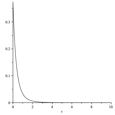
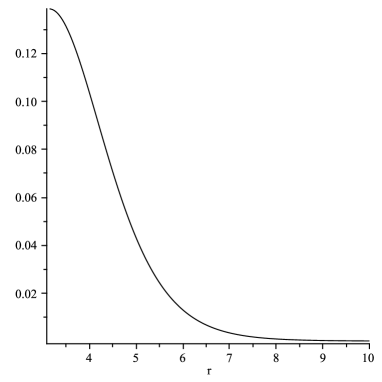
Figure 1: The density (8.14) for TN (left) and AH (right)

8.3 Electric and baryonic fluxes

We now construct fields on TN and AH which carry the electric flux measured by the self-intersection numbers $X^{2}$ tabulated in Table 1. We do this by systematically studying rotationally symmetric harmonic forms on both TN and AH, with most of the details given in Appendix C.

One finds [28, 29, 30, 31] that the only square-integrable harmonic and rotationally symmetric 2-form on TN is, up to an overall arbitrary constant,

$$\omega_{3}^{+}=\left(\frac{r}{r+2}\,\eta_{1}\wedge\eta_{2}+\frac{2}{(r+2)^{2}}\,dr\wedge\eta_{3}\right)=d\left(\frac{r}{r+2}\,\eta_{3}\right)\,.$$ (8.16)

We claim that this form is a harmonic representative of the Poincaré dual of the surface $X=\mathbb{CP}^{1}$ at infinity in TN, the surface parametrised by $\theta$ and $\phi$. Our calculation also gives an alternative computation of the electric charge as minus the self-intersection number of $\mathbb{CP}^{1}$ in $\mathbb{CP}^{2}$. Let $p$ be this self-intersection number, then

$$\omega_{\mathbb{CP}^{1}}=-\frac{p}{4\pi}\,\omega_{3}^{+}$$ (8.17)

is Poincaré dual to $\mathbb{CP}^{1}$ since

$$\int_{\mathbb{CP}^{1}}\omega_{\mathbb{CP}^{1}}=p\,.$$ (8.18)

However, by the definition of the self-intersection numbers in terms of cohomology, we also have

$$\int_{{\rm TN}}\omega_{\mathbb{CP}^{1}}\wedge\omega_{\mathbb{CP}^{1}}=p\,.$$ (8.19)

Evaluating the integral in Appendix C we find

$$p^{2}=p\,,$$ (8.20)

so that $p=1$, confirming that, with the self-dual orientation, the self-intersection of $\mathbb{CP}^{1}$ in $\mathbb{CP}^{2}$ is 1.

Since the 2-form $-\omega_{\mathbb{CP}^{1}}$ is harmonic and since its total flux through infinity equals the electric charge we interpret it as the electric field of the electron. Although we have adopted a viewpoint dual to standard electromagnetism, with a purely spatial 2-form being interpreted as electric rather than magnetic flux, it is interesting that the self-dual 2-form (8.16) also contains a term which allows for a conventional electric interpretation: when we contract $\omega_{\mathbb{CP}^{1}}$ with the vector field $\partial_{\psi}$ along the fibres (using $\eta_{3}(\partial_{\psi})=1$), we obtain a purely radial field which, asymptotically, falls off like $1/r^{2}$.

The integral (8.19) is the squared $L^{2}$-norm of the electric field. Ignoring overall factors and working with $\omega_{3}^{+}$ we write

$$||\omega_{3}^{+}||^{2}=\int\rho_{3}^{+}\,dV\,,$$ (8.21)

with $dV$ defined as in (B.17), and interpret the integrand

$$\rho_{3}^{+}(r)=\frac{2}{(r+2)^{4}}$$ (8.22)

as an electric energy density. For comparison with the AH case below, we plot the profile function $g_{3}^{+}(r)=r/(r+2)$ and the energy density $\rho_{3}^{+}$ in Fig. 2.

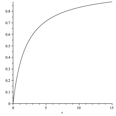
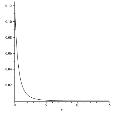
Figure 2: The ‘electric’ profile function $g_{3}^{+}$ and the energy density $\rho_{3}^{+}$

Turning now to AH, we review in Appendix C why there are only two $SO(3)$-invariant harmonic forms $\Omega^{\pm}_{1}$ on AH which respect the identification (B.7). They have the structure

$$\Omega^{\pm}_{1}=G^{\pm}_{1}\eta_{2}\wedge\eta_{3}+dG^{\pm}_{1}\wedge\eta_{1}\,,$$ (8.23)

for functions $G^{\pm}_{1}$ of $r$ which satisfy the ordinary differential equations for $g^{\pm}_{1}$ in (C.1). Using the asymptotic formulae (C.13) and (C.14) one shows [24, 32, 33] that only $G^{+}_{1}$ is finite at the core and decays at infinity. In fact, the solution decays exponentially fast at infinity, with the leading term proportional to $e^{-r/2}$. We normalise $G_{1}^{+}(\pi)=1$, so that near the core

$$G_{1}^{+}(r)\sim 1-\frac{1}{\pi^{2}}(r-\pi)^{2}\,,\quad\text{for}\;(r-\pi)\;\text{small}\,.$$ (8.24)

The 2-form $\Omega^{+}_{1}$ is not dual to the surface $X=\mathbb{RP}^{2}$ at infinity in AH and has no interpretation in terms of electric flux. However, it is dual to the core $\mathbb{CP}^{1}$ in AH. With

$$\Omega_{{\rm core}}=-\frac{p}{4\pi}\Omega_{1}^{+}$$ (8.25)

one finds

$$\int_{{\rm core}}\Omega_{{\rm core}}=p\,.$$ (8.26)

As a check, we use this form to compute the self-intersection number of the core. Recalling that the volume of $SO(3)/\mathbb{Z}_{2}$ is $-4\pi^{2}$, and using (C.3), we have

$$\int_{{\rm AH}}\Omega_{{\rm core}}\wedge\Omega_{{\rm core}}=\frac{p^{2}}{16\pi^{2}}(-4\pi^{2})(0^{2}-1^{2})=\frac{p^{2}}{4}\,,$$ (8.27)

so that

$$\frac{p^{2}}{4}=p\,,$$ (8.28)

confirming $p=4$ for the self-dual orientation (this agrees with [13], where the anti-self-dual orientation gives the opposite sign).

The harmonic form (4.8) on $\mathbb{CP}^{2}$ is related to the signature of $\mathbb{CP}^{2}$ through the fact that the signature of a compact 4-manifold equals the difference of the dimensions of the spaces of self-dual and anti-self-dual harmonic representatives of the second de Rham cohomology. It seems likely that the (up to scale) unique bounded and rotationally symmetric self-dual harmonic form $\Omega_{{\rm core}}$ on AH is related to the self-dual harmonic form (4.8) via the sequence of Hitchin manifolds reviewed in Sect. 4.2.

Since the existence of $\Omega_{{\rm core}}$ on AH is linked to the signature of AH being 1, and since signature represents baryon number in our approach, it may be possible to interpret the detailed structure of $\Omega_{{\rm core}}$ in baryonic terms. The exponential fall-off exhibited by $\Omega_{{\rm core}}$ is reminiscent of the proton’s pion field in the Yukawa description of the nuclear force. In Fig. 3 we plot the numerically computed profile function $G_{1}^{+}$ and the associated energy density (C.17), which turns out to be

$$\rho_{1}^{+}=2\frac{(G_{1}^{+})^{2}}{b^{2}c^{2}}\,.$$ (8.29)

This is finite at the core and decays exponentially according to $e^{-r}$ for large $r$.

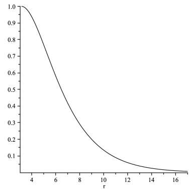
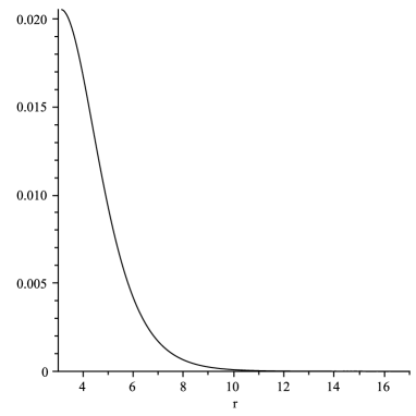
Figure 3: The ‘baryonic’ profile function $G_{1}^{+}$ and the energy density $\rho_{1}^{+}$

To find a harmonic 2-form on AH which can play the role of the proton’s electric field we need to go to a branched cover of AH, denoted $\overline{\rm AH}$. The metric on the branched cover is not smooth at the core, but this will not affect the following calculations near infinity. Dropping the requirement that forms are invariant under the identification (B.7), we find that the closure condition on the 2-forms (C.3) has only one further solution which is finite at the core and which remains bounded for large $r$. This is the 2-form

$$\Omega^{-}_{3}=G^{-}_{3}\eta_{1}\wedge\eta_{2}+dG^{-}_{3}\wedge\eta_{3}\,,$$ (8.30)

with a radial function $G_{3}^{-}$ satisfying (C.1). The solution vanishes at the core as

$$G_{3}^{-}(r)\sim C\sqrt{r-\pi}\,,\quad\text{for}\;(r-\pi)\;\text{small}\,,$$ (8.31)

for some constant $C$. The large $r$ behaviour is

$$G_{3}^{-}(r)\sim\widetilde{C}\,\frac{r-2}{r}\,,$$ (8.32)

where $\widetilde{C}$ is another constant. This leads to an anti-self-dual form on $\overline{\rm AH}$, which is square-integrable (as we shall show below) and which has not been considered previously. It is our candidate for the electric field of the proton.

As a manifold, $\overline{\rm AH}$ compactifies to $S^{2}\times S^{2}$, as discussed in Appendices A.4 and A.5. The surface $X=\mathbb{RP}^{2}$ which compactifies AH to $\mathbb{CP}^{2}$ becomes the anti-diagonal $S^{2}$ in $S^{2}\times S^{2}$. Choosing $\widetilde{C}=1$ in (8.32), a harmonic representative of the Poincaré dual class to this $S^{2}$ is

$$\Omega_{S^{2}}=-\frac{p}{4\pi}\,\Omega_{3}^{-}\,.$$ (8.33)

Then

$$\int_{S^{2}}\Omega_{S^{2}}=p\,,$$ (8.34)

and since the volume of $SO(3)$ is $-8\pi^{2}$ by (B.1), we also compute

$$\int_{\overline{\rm AH}}\Omega_{S^{2}}\wedge\Omega_{S^{2}}=\frac{p^{2}}{16\pi^{2}}(-8\pi^{2})(1^{2}-0^{2})=-\frac{p^{2}}{2}\,.$$ (8.35)

Hence

$$-\frac{p^{2}}{2}=p\,,$$ (8.36)

which is solved by $p=-2$. Dividing by 2, to take us back to $\mathbb{RP}^{2}$, we confirm the self-intersection number of $\mathbb{RP}^{2}$ in $\mathbb{CP}^{2}$ as $-1$, again for the self-dual orientation.

Since the 2-form $-\Omega_{S^{2}}$ on $\overline{\rm AH}$ is harmonic and since its total flux through infinity, suitably interpreted, equals the electric charge, we think of $-\Omega_{S^{2}}$ as representing the electric field of the proton. The comments made after (8.16) about the possibility of recovering a conventional electric field by contracting the electric 2-form on TN with the vector field along asymptotic fibres apply, suitably modified, to $\overline{\rm AH}$.

In Fig. 4 we plot the numerically computed profile function $G_{3}^{-}$ for $C=1$ (as defined in (8.31)) and the associated energy density (C.17), which turns out to be

$$\rho_{3}^{-}=2\frac{(G_{3}^{-})^{2}}{a^{2}b^{2}}\,.$$ (8.37)

This function has a $(r-\pi)^{-1}$ singularity at $r=\pi$, and falls off like $r^{-4}$ for large $r$ as in the TN case.

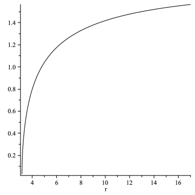
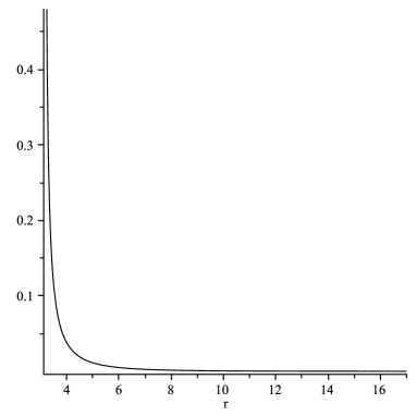
Figure 4: The ‘electric’ profile function $G_{3}^{-}$ and the energy density $\rho_{3}^{-}$

9 Conclusion and outlook

In introducing and illustrating geometric models of matter in this paper we have concentrated on general, global properties of particles like baryon number and electric charge. The most striking phenomenological success of our geometric approach is its prediction of precisely two stable electrically charged particles, one leptonic and one baryonic, with opposite electric charges.

An important theme throughout this paper is the implementation of rotational symmetry in our models. The rotation action preserves the metric and, in the compact cases, the distinguished surface where the 4-manifold intersects physical 3-space. We have shown that our models are fermionic in the sense that the lift of the rotation action to spin bundles (over the ‘inside’ of the 4-manifold in the compact cases) is necessarily an $SU(2)$-action, but we have left the explicit construction of spin 1/2 states for future work.

Non-vanishing electric charge and baryon number give rise to harmonic 2-forms on our model manifolds. These have allowed us to make contact with the conventional description of charged particles in terms of associated fields and fluxes.

There are various geometrically natural candidates for measuring energy or mass in our models, but we have not committed ourselves to any particular energy functional in this paper. In the absence of an energy measure, we are not able to make contact with experimental data about particle masses or forces between particles.

We end our summary with some observations about relative scales predicted by our models for charged particles. The AH model relates three scale parameters: the size of the core (radius $\approx\pi$ in our geometric units), the size of the asymptotic circles (radius 2 in geometric units) and the scale $1$ implicit in the exponential corrections to the asymptotic form of the coefficient functions (3.7) for the AH metric, which are proportional to $e^{-r}$ (see [34, 35] for a discussion of these corrections in the context of magnetic monopoles). Interpreting the core radius as the proton radius and the scale in the exponential decay as the Compton wavelength $\lambda_{\pi}$ of the pion, we find that our model correctly assigns the same order of magnitude to those two quantities. The details are not quite right (experimentally, the proton radius is just over half of $\lambda_{\pi}$) but this is not surprising given our very rudimentary understanding of how our model relates to experiment. In any case, these considerations suggest that we should pick a length unit of about 1 fermi or $10^{-15}$ m in the AH model.

Since the asymptotic fibration by circles arises for all electrically charged particles, we expect the size of the asymptotic circle to have a purely electric interpretation, and we also assume that it is the same for both AH and TN (this was implicit in the way we fixed scale and units for TN). One natural guess, at least for TN, is to relate the size of the asymptotic circle to the classical electron radius. Our models would then equate the orders of magnitude of the classical electron radius with the Compton wavelength of the pion, which is phenomenologically right. It is an attractive feature of TN as a model for the electron that it has a length scale, but no core structure.

Many avenues remain to be explored. In our geometric approach, fusion and fission of nuclei as well as decay processes involving both baryons and leptons (like the beta decay of the neutron) should have a description in terms of gluing and deformation of self-dual 4-manifolds. In order to study masses and binding energies of particles we need to pick an energy measure. This could involve the norms of curvatures and harmonic forms discussed here, but may take a less conventional form. Our ideas about spin 1/2 need to be fleshed out. The Dirac operator on our model manifolds is likely to play a role in combining energy and spin considerations, and Seiberg-Witten theory on the model manifolds seems relevant, too. In order to move beyond static consideration, time needs to be introduced.

The list of open issues may seem daunting, but in each case the geometric framework introduced here suggests natural lines of attack. We hope to pursue them in future work.

Acknowledgment   We thank Nigel Hitchin and Claude LeBrun for assistance and José Figueroa-O’Farrill for working with us during the early stages of the project.

Appendices

Appendix A Geometry and sign conventions

A.1 Self-intersection numbers

Let $L$ be a complex line bundle over a compact oriented surface $X$. Then

$$c_{1}(L)[X]=X^{2}$$ (A.1)

where $X^{2}$ denotes the self-intersection number of the zero section in the total space of $L$. This is essentially one of the definitions of the first Chern class. Note that both $X$ and $L$ are oriented, with the fibres having the natural orientation of the complex numbers. However the self-intersection $X^{2}$ depends only on the orientation of the total space, since $(-X)^{2}=X^{2}$.

A.2 The Hopf bundle

Let us review the definition of the Hopf bundle $H$, the standard line bundle over the complex projective line, paying particular attention to orientations. We start with $\mathbb{C}^{2}$, and $\mathbb{CP}^{1}$ as the space of complex lines through the origin. This complex line bundle is defined to be the dual of the line bundle $H$. The reason for this apparently perverse choice is that $H$ has holomorphic sections (given by $\mathbb{C}^{2}$) and its dual $H^{*}$ does not. This is clear from the exact sequence of holomorphic vector bundles over $\mathbb{CP}^{1}$:

$$0\rightarrow H^{*}\rightarrow\mathbb{C}^{2}\rightarrow H\rightarrow 0\,.$$ (A.2)

Since holomorphic intersections are always positive, the first Chern class of $H$ gives $+1$ when evaluated on the fundamental class of $\mathbb{CP}^{1}$.

If we compactify $\mathbb{C}^{2}$ by adding a $\mathbb{CP}^{1}$ at infinity then the self-intersection number of this line is clearly $+1$, so that the normal bundle is $H$.

A.3 Non-orientable surfaces

Now assume that $X$ is a non-orientable surface in an oriented 4-manifold $M$. This defines a mod 2 homology class in $M$ and so it would appear that its self-intersection number is only defined modulo 2. However a more careful look shows that we can define an integer self-intersection. There are several (equivalent) ways to see this. First we note that the tangent bundle and the normal bundle of $X$ in $M$ have isomorphic orientation real line bundles $L$. Then both the Euler class of the normal bundle and the fundamental class of $X$ are defined as classes ‘twisted’ by $L$. The evaluation (A.1) therefore makes sense and defines $X^{2}$. An alternative way is to pass to the double covering of a neighbourhood of $X$ in $M$, where $X$ acquires an orientation, compute the self-intersection there and divide by 2. A third way is to deform $X$ into a transverse surface $\widetilde{X}$ and, near each intersection point of $X$ and $\widetilde{X}$, choose an orientation of $X$ and the corresponding orientation of $\widetilde{X}$ given by the deformation. Now compute the local intersection numbers of $X$ and $\widetilde{X}$ and sum them up.

A.4 An example

The example we want to study is that of the real projective plane $X=\mathbb{RP}^{2}$ inside the complex projective plane $M=\mathbb{CP}^{2}$. We give $M$ its standard complex orientation. We plan to show that $X^{2}=-1$.

To do this we will use the double branched covering of $\mathbb{CP}^{2}$ given by the product of two copies of the complex projective line $\mathbb{CP}^{1}$. We can identify $\mathbb{CP}^{2}$ with the symmetric product of the two copies, branched along the diagonal $D$. This map is holomorphic and compatible with the action of $SL(2,\mathbb{C})$. Now introduce a metric on $\mathbb{CP}^{1}$ identifying it with a 2-sphere, and consider in $\mathbb{CP}^{1}\times\mathbb{CP}^{1}$ the graph $D^{\prime}$ of the antipodal map. The image of $D^{\prime}$ in $\mathbb{CP}^{2}$ is the standard embedding of $\mathbb{RP}^{2}$ into $\mathbb{CP}^{2}$. Outside the branch locus $D$ the map from the product of the two 2-spheres to $\mathbb{CP}^{2}$ is a double covering so we can compute $X^{2}$ as half of $(D^{\prime})^{2}$. This is most easily done by observing that, in the cohomology of the product, with $x$ and $y$ the two generators of $H^{2}$, the classes of $D$ and $D^{\prime}$ are

$$D=x+y\,,\quad D^{\prime}=x-y\,.$$ (A.3)

Since $x^{2}=y^{2}=0$ and $xy=1$ it follows that

$$D^{2}=2\quad\text{and}\quad(D^{\prime})^{2}=-2$$ (A.4)

(while $D.D^{\prime}=0$ agreeing with the fact that $D$ and $D^{\prime}$ are disjoint). Dividing by 2 to get back down to $\mathbb{CP}^{2}$ we end up with $X^{2}=-1$ as stated.

As a check we can also use a deformation of $D^{\prime}$ in $M$ by choosing a different metric on $\mathbb{CP}^{1}$ giving a different antipodal map. In particular, consider the 2-sphere as the boundary of the unit ball in $\mathbb{R}^{3}$ and move the origin so that antipodal points are now the end points of lines through the new origin. The line joining the two origins defines a unique intersection point of the two copies of $\mathbb{RP}^{2}$ in $\mathbb{CP}^{2}$. Since this line acquires different orientations from the two origins the intersection number is $-1$.

A third sign check is to observe that the normal bundle to the diagonal in the product of the two 2-spheres is the tangent bundle with Euler number 2, while for the antidiagonal (graph of the antipodal map) it is the cotangent bundle with Euler number $-2$.

A.5 More on the example

It is enlightening to analyze the $SO(3)$ action on the spaces in the example above. In addition we can introduce the branched double covering $\mathbb{CP}^{2}\rightarrow S^{4}$ given by complex conjugation [36, 37]. This is branched over $\mathbb{RP}^{2}$.

Thus we have maps

$$S^{2}\times S^{2}\rightarrow\mathbb{CP}^{2}\rightarrow S^{4}\,,$$ (A.5)

which are compatible with the $SO(3)$ actions. Here $S^{4}$ is best thought of as the space of real $3\times 3$ symmetric matrices of zero trace and fixed norm.

The generic orbits are, in each case, 3-dimensional but there are two exceptional orbits of dimension 2. Inside the product $S^{2}\times S^{2}$ they are the diagonal and anti-diagonal (both $S^{2}$), in $S^{4}$ they are both $\mathbb{RP}^{2}$, while in $\mathbb{CP}^{2}$ one is $S^{2}$ and one is $\mathbb{RP}^{2}$. Each of the two maps is branched along a surface: $S^{2}$ for the first map and $\mathbb{RP}^{2}$ for the second.

To examine the self-intersection numbers of the exceptional orbits it is useful to note two general rules:

1. If $X$ in $M$ is double covered by $X^{\prime}$ in $M^{\prime}$ then $(X^{\prime})^{2}=2X^{2}$.

2. If $X$ is a branch locus in the double covering then $(X^{\prime})^{2}=\frac{1}{2}X^{2}$.

Rule A is obvious and rule B is familiar in algebraic geometry, but it applies more generally even in the non-orientable case.

Using rules A and B we can now check what happens in our two maps. In $S^{4}$ the two $\mathbb{RP}^{2}$s have self-intersection numbers $+2$ and $-2$. In $S^{2}\times S^{2}$ the two 2-spheres also have self-intersection numbers $+2$ and $-2$. In $\mathbb{CP}^{2}$ the 2-sphere, which is a conic, has self-intersection number $+4$, while $\mathbb{RP}^{2}$ has self-intersection number $-1$.

A.6 Self-dual manifolds

We want to analyze various sign conventions in relation to self-dual manifolds, and begin by checking our sign conventions for two examples of complex Kähler surfaces. Referring to our discussion of the signature and Euler characteristic in Sect. 8.2, we note the examples:

1. The K3 surface with the Yau metric, which makes it hyperkähler. With its complex orientation its signature is $-16$ and its Euler characteristic is 24. With the opposite orientation, the metric is self-dual and the signature is positive.

2. $\mathbb{CP}^{2}$ with the Fubini-Study metric is self-dual for its complex orientation [12], agreeing with the positive signature $+1$.

We will also be interested in non-compact examples similar to the above. The argument that a hyperkähler manifold is self-dual for the orientation opposite to the complex orientation (given by one of the family of complex Kähler structures) is purely local. It just depends on the fact that the bundle of self-dual 2-forms for these complex orientations is flat. More generally, on any Kähler manifold, the bundle of self-dual 2-forms is the direct sum of the canonical line bundle $K$, its dual and a trivial bundle generated by the Kähler form.

The first non-compact example that interests us is the Taub-NUT manifold TN. This has the isometry group $U(2)$, its topology (and symmetry) is that of $\mathbb{C}^{2}$ with the central $U(1)$ giving the scalar action. The other $U(1)$ actions, inside $SU(2)$, define the complex hyperkähler structures which have the opposite orientation. Hence TN is self-dual for the orientation that becomes that of $\mathbb{C}^{2}$ in the limit when the parameter $\epsilon$ goes to 0, as discussed after (3.5).

The second example is that of the (simply-connected version of the) Atiyah-Hitchin manifold AH, which is an open subspace of $\mathbb{CP}^{2}$ got by removing $\mathbb{RP}^{2}$. As shown in [13], it has a complete hyperkähler metric. This is self-dual for the orientation opposite to the complex orientations given by the hyperkähler metric. But this is just the orientation given by its complex structure as an open subset of $\mathbb{CP}^{2}$. This can be checked directly, but it is best seen by using the results of Hitchin [21], reviewed in Sect. 4.2, which give a whole sequence of self-dual manifolds on the same space, starting from the Fubini-Study metric of $\mathbb{CP}^{2}$ and converging to AH.

In each case, for TN and AH, we have a hyperkähler manifold acted on by $SU(2)$ (the action descends to $SO(3)$ for AH). The manifolds have a ‘core region’ and an ‘asymptotic region’ with an asymptotic action of $O(2)$. In addition to the 2-parameter family of complex structures given by the hyperkähler metric (and rotated by $SU(2)$) there is another complex structure compatible with the $SU(2)$ action, but giving the opposite orientation to that of the 2-parameter family. For TN this complex manifold is just $\mathbb{C}^{2}$ and for AH it is $\mathbb{CP}^{2}\setminus\mathbb{RP}^{2}$.

In both cases the asymptotic $O(2)$ action gives us topologically a disc bundle at infinity and this can be identified with the normal bundle of the surface $X$ that naturally compactifies the manifold. For TN this compactification is $\mathbb{CP}^{2}$ with $X=\mathbb{CP}^{1}$, and for AH it is $\mathbb{CP}^{2}$ with $X=\mathbb{RP}^{2}$. We have shown that these give rise to opposite signs:

$$\mbox{For TN}\quad X^{2}=+1\quad\mbox{while for AH}\quad X^{2}=-1\,.$$

As explained in the main text, TN and AH are our geometric models for the electron and the proton, and we identify the self-intersection number of $X$ with minus the electric charge.

Appendix B Metric properties of TN and AH

B.1 Coordinates and conventions

In this paper we need to parametrise $SU(2)$ explicitly at various points, and we use generators

$$t_{1}=\frac{1}{2}i\tau_{1}=\frac{1}{2}\begin{pmatrix}0&i\\ i&0\end{pmatrix}\,,\quad t_{2}=\frac{1}{2}i\tau_{2}=\frac{1}{2}\begin{pmatrix}\phantom{-}0&1\\ -1&0\end{pmatrix}\,,\quad t_{3}=\frac{1}{2}i\tau_{3}=\frac{1}{2}\begin{pmatrix}i&\phantom{-}0\\ 0&-i\end{pmatrix}\,,$$ (B.1)

where $\tau_{a}$, $a=1,2,3$, are the Pauli matrices; the commutators are $[t_{a},t_{b}]=-\epsilon_{abc}t_{c}$. We use Euler angles $\theta\in[0,\pi)$, $\phi\in[0,2\pi)$ and $\psi\in[0,4\pi)$ for parametrising $SU(2)$ as follows:

$$g(\phi,\theta,\psi)=e^{\phi t_{3}}e^{\theta t_{2}}e^{\psi t_{3}}=\begin{pmatrix}e^{\frac{i}{2}(\psi+\phi)}\cos\frac{1}{2}\theta&e^{\frac{i}{2}(\phi-\psi)}\sin\frac{1}{2}\theta\\ -e^{\frac{i}{2}(\psi-\phi)}\sin\frac{1}{2}\theta&e^{-\frac{i}{2}(\psi+\phi)}\cos\frac{1}{2}\theta\end{pmatrix}.$$ (B.2)

Defining left-invariant 1-forms $\eta_{a}$ on $SU(2)$ via

$$g^{-1}dg=\eta_{1}t_{1}+\eta_{2}t_{2}+\eta_{3}t_{3}\,,$$ (B.3)

we compute to find

$$\eta_{1} \ =\ -\sin\psi\,d\theta+\cos\psi\sin\theta\,d\phi\,,$$

$$\eta_{2} \ =\ \phantom{-}\cos\psi\,d\theta+\sin\psi\sin\theta\,d\phi\,,$$

$$\eta_{3} \ =\ \phantom{-}\,d\psi+\cos\theta\,d\phi\,,$$ (B.4)

satisfying $d\eta_{i}=\frac{1}{2}\epsilon_{ijk}\eta_{j}\wedge\eta_{k}$. They descend to $SO(3)$ by simply restricting $\psi$ to $[0,2\pi)$.

Explicitly, generators of the Lie algebra of $SO(3)$ are $(T_{a})_{bc}=\epsilon_{abc}$. They also satisfy $[T_{a},T_{b}]=-\epsilon_{abc}T_{c}$. We can then parametrise $SO(3)$ matrices via

$$R(\phi,\theta,\psi)=e^{\phi T_{3}}e^{\theta T_{2}}e^{\psi T_{3}},$$ (B.5)

with $\theta\in[0,\pi)$, $\phi\in[0,2\pi)$ and $\psi\in[0,2\pi)$. Then

$$R^{-1}dR=\eta_{1}T_{1}+\eta_{2}T_{2}+\eta_{3}T_{3}$$ (B.6)

provides an alternative definition of the left-invariant 1-forms on $SO(3)$: one obtains the same expressions as in (B.1), but with the range of angles automatically appropriate to $SO(3)$.

Both TN and AH can be parametrised in terms of Euler angles and a radial coordinate. For TN, the angular ranges are $\theta\in[0,\pi)$, $\phi\in[0,2\pi)$ and $\psi\in[0,4\pi)$. For AH they are $\theta\in[0,\pi)$, $\phi\in[0,2\pi)$ and $\psi\in[0,2\pi)$ with the additional $\mathbb{Z}_{2}$ identification

$$(\theta,\phi,\psi)\simeq(\pi-\theta,\phi+\pi,-\psi),$$ (B.7)

which, in the asymptotic region, is the simultaneous reversal of spatial and fibre direction. The following angular integrals, which enter into various calculations in this paper, are therefore

$$\int_{SU(2)}\eta_{1}\wedge\eta_{2}\wedge\eta_{3} =-16\pi^{2}\,,$$

$$\int_{SO(3)}\eta_{1}\wedge\eta_{2}\wedge\eta_{3} =-8\pi^{2}\,,$$

$$\int_{(SO(3)/\mathbb{Z}_{2})}\eta_{1}\wedge\eta_{2}\wedge\eta_{3} =-4\pi^{2}\,.$$ (B.8)

Note that $\eta_{1}$ is invariant under (B.7), but $\eta_{2}$ and $\eta_{3}$ change sign.

Recalling that the metrics on TN and AH are of the Bianchi IX form

$$ds^{2}=f(r)^{2}dr^{2}+a(r)^{2}\eta_{1}^{2}+b(r)^{2}\eta_{2}^{2}+c(r)^{2}\eta_{3}^{2}\,,$$ (B.9)

we introduce the tetrad

$$\theta^{1}=a\eta_{1}\,,\;\theta^{2}=b\eta_{2}\,,\;\theta^{3}=c\eta_{3}\,,\;\theta^{4}=fdr\,.$$ (B.10)

The self-duality of the Riemann tensor computed from (B.9) with respect to the volume element

$$dV=a\eta_{1}\wedge b\eta_{2}\wedge c\eta_{3}\wedge fdr=-fabc\,dr\wedge\eta_{1}\wedge\eta_{2}\wedge\eta_{3}$$ (B.11)

is then equivalent to the set of ordinary differential equations

$$\frac{2bc}{f}\frac{da}{dr}=(b-c)^{2}-a^{2}+2\lambda bc\,,\qquad\mbox{+ cyclic}\,,$$ (B.12)

where ‘+ cyclic’ means we add the two further equations obtained by cyclic permutation of $a,b,c$, and $\lambda$ is a parameter which has to be either $0$ or $1$. In all cases the resulting metrics are hyperkähler, but in order to obtain metrics whose hyperkähler structures are rotated by the $SU(2)$ action we need to set $\lambda=0$. This is the case for both TN and AH, so $\lambda=0$ in (B.12).

One checks the equivalence of the self-duality of the Riemann tensor and (B.12) as follows. Denoting the Riemann tensor by $R$, its component 2-forms with respect to (B.10) are

$$R_{12} =d\mu_{3}\wedge\eta_{3}+(\mu_{3}-\mu_{1}\mu_{2}-\lambda_{1}\lambda_{2})\eta_{1}\wedge\eta_{2}\,,$$

$$R_{34} =d\lambda_{3}\wedge\eta_{3}+(\lambda_{3}-\lambda_{1}\mu_{2}-\lambda_{2}\mu_{1})\eta_{1}\wedge\eta_{2}\,,$$ (B.13)

and similar expressions for the components obtained by cyclic permutation of $1,2,3$, where

$$\mu_{1}=\frac{b^{2}+c^{2}-a^{2}}{2bc}\,,\quad\mu_{2}=\frac{c^{2}+a^{2}-b^{2}}{2ca}\,,\quad\mu_{3}=\frac{a^{2}+b^{2}-c^{2}}{2ab}$$ (B.14)

and

$$\lambda_{1}=\frac{1}{f}\frac{da}{dr}\,,\quad\lambda_{2}=\frac{1}{f}\frac{db}{dr}\,,\quad\lambda_{3}=\frac{1}{f}\frac{dc}{dr}\,.$$ (B.15)

When (B.12) hold, then $\lambda_{i}=\mu_{i}+\lambda-1$, $i=1,2,3$, with $\lambda=0$ or $\lambda=1$, and the self-duality relations

$$R_{12}=R_{34}\,,\quad R_{23}=R_{14}\,,\quad R_{31}=R_{24}$$ (B.16)

are easily verified. One also checks that each of the three independent 2-forms $R_{12},R_{23},R_{31}$ is self-dual with respect to (B.11), as expected.

The only solutions of (B.12) with $\lambda=0$ which give rise to complete manifolds whose generic $SU(2)$- or $SO(3)$-orbit is three-dimensional are the TN and AH metrics, whose coefficient functions we discussed in Sect. 3. It is important that the coefficient function $c$ in (3.1) is negative for all $r$ in the AH manifold. It implies in particular that the canonical volume element/orientation $dV$ in (B.11), with $f=-b/r$,

$$dV=-fabc\,dr\wedge\eta_{1}\wedge\eta_{2}\wedge\eta_{3}=-\frac{ab^{2}c}{r}\sin\theta\,dr\wedge d\theta\wedge d\phi\wedge d\psi\,,$$ (B.17)

has opposite signs for TN and AH, in the following sense. Assuming the same orientation $\eta_{1}\wedge\eta_{2}\wedge\eta_{3}$ of the $SU(2)$ and $SO(3)$ orbits in TN and, respectively, AH, the radial direction is oppositely oriented in the two cases: the natural radial line element $-fabc\,dr$ has the same orientation as $dr$ for TN, but the opposite orientation for AH. This will be important when evaluating various integrals. It means that, when using the coordinates $r,\theta,\phi,\psi$ we can use the conventional orientations for these coordinates when computing for AH, but should use the opposite orientation when computing for TN. Thus we integrate in the negative $r$-direction when calculating on TN.

B.2 $L^{2}$-norms of the Riemann curvature

The squared $L^{2}$-norm of the Riemann tensor is

$$||R||_{M}^{2}=\int_{M}2(R_{12}\wedge R_{12}+R_{23}\wedge R_{23}+R_{31}\wedge R_{31})\,,$$ (B.18)

where $M$ is TN or AH, and we have used the self-duality of the curvature. In terms of the functions (B.14) the integrand can be simplified (see also [38], where this calculation is carried out for the AH metric) and becomes

$$2(R_{12}\wedge R_{12}+R_{23}\wedge R_{23}+R_{31}\wedge R_{31})=dF\wedge\eta_{1}\wedge\eta_{2}\wedge\eta_{3},$$ (B.19)

with

$$F=2(\mu_{1}+\mu_{2}+\mu_{3}-1)^{2}-8\mu_{1}\mu_{2}\mu_{2}\,.$$ (B.20)

We denote these functions in the TN and AH cases by $F_{{\rm TN}}$ and $F_{{\rm AH}}$.

For TN, we can compute explicitly and find

$$F_{{\rm TN}}(r)=-8\,\frac{2r+1}{(r+2)^{4}}\,.$$ (B.21)

Integrating (B.19) and using (B.1) as well as our sign convention for the volume form we find

$$||R||^{2}_{{\rm TN}}=(-16\pi^{2})(F_{{\rm TN}}(0)-F_{{\rm TN}}(\infty))=8\pi^{2}\,.$$ (B.22)

For AH, similarly,

$$||R||^{2}_{{\rm AH}}=(-4\pi^{2})(F_{{\rm AH}}(\infty)-F_{{\rm AH}}(\pi))\,.$$ (B.23)

To complete the calculation we need the behaviour of $F_{{\rm AH}}$ at infinity and at $\pi$. One finds for AH

$$\mu_{1}(\infty)=\mu_{2}(\infty)=\frac{c}{2a}\left(\infty\right)=0\,,\quad\mu_{3}(\infty)=1-\frac{c^{2}}{2a^{2}}\left(\infty\right)=1\,,$$ (B.24)

as well as

$$\mu_{1}(\pi)=-1\,,\quad\mu_{2}(\pi)=\frac{1}{2}\,,\quad\mu_{3}(\pi)=\frac{1}{2}\,,$$ (B.25)

where we took careful limits, using (3.7) and (3.8). Therefore

$$F_{{\rm AH}}(\infty)=0\,,\qquad F_{{\rm AH}}(\pi)=4\,,$$ (B.26)

so

$$||R||^{2}_{{\rm AH}}=(-4\pi^{2})\times(0-4)=16\pi^{2}\,.$$ (B.27)

Appendix C Harmonic forms on TN and AH

C.1 Rotationally symmetric harmonic forms

The question of computing harmonic 2-forms on the TN and AH manifolds arose in physics in the context of testing S-duality, see [33] for AH and [30, 31] for TN. Harmonic forms also play a role as curvatures of line bundles over TN and AH, see [32] for a discussion of this for AH where the form later used for testing S-duality [33] is the curvature of an index bundle. This appendix contains a systematic discussion of these forms and also a harmonic form on the branched cover of AH which has not previously been considered in the literature. The physical interpretation of the forms as electric and baryonic fluxes is given in Sect. 8.

On both TN and AH, rotationally symmetric 2-forms can be written in terms of the metric coefficient functions $f,a,b,c$ appearing in the respective metrics and functions $f_{1},f_{2}$ and $f_{3}$ of the radial coordinate $r$ as

$$\omega^{\pm}_{1} =f^{\pm}_{1}\left(b\eta_{2}\wedge c\eta_{3}\pm a\eta_{1}\wedge fdr\right)\,,$$

$$\omega^{\pm}_{2} =f^{\pm}_{2}\left(c\eta_{3}\wedge a\eta_{1}\pm b\eta_{2}\wedge fdr\right)\,,$$

$$\omega^{\pm}_{3} =f^{\pm}_{3}\left(a\eta_{1}\wedge b\eta_{2}\pm c\eta_{3}\wedge fdr\right)\,,$$ (C.1)

with $+$ standing for self-dual and $-$ standing for anti-self-dual. Introducing the functions

$$g_{1}^{\pm}=f_{1}^{\pm}bc\,,\quad g_{2}^{\pm}=f_{2}^{\pm}ca\,,\quad g_{3}^{\pm}=f_{3}^{\pm}ab\,,$$ (C.2)

closure of the forms (C.1) implies the ordinary differential equations

$$\frac{dg_{1}^{\pm}}{dr} =\mp\frac{af}{bc}g_{1}^{\pm}\,,$$

$$\frac{dg_{2}^{\pm}}{dr} =\mp\frac{bf}{ca}g_{2}^{\pm}\,,$$

$$\frac{dg_{3}^{\pm}}{dr} =\mp\frac{cf}{ab}g_{3}^{\pm}\,.$$ (C.3)

For solutions of these differential equations (we shall discuss below in which cases regular solutions exist), the forms (C.1) can be written

$$\omega^{\pm}_{1} =g^{\pm}_{1}\eta_{2}\wedge\eta_{3}+dg^{\pm}_{1}\wedge\eta_{1}\,,$$

$$\omega^{\pm}_{2} =g^{\pm}_{2}\eta_{3}\wedge\eta_{1}+dg^{\pm}_{2}\wedge\eta_{2}\,,$$

$$\omega^{\pm}_{3} =g^{\pm}_{3}\eta_{1}\wedge\eta_{2}+dg^{\pm}_{3}\wedge\eta_{3}\,.$$ (C.4)

All these forms are locally exact, that is,

$$\omega^{\pm}_{i}=d(g^{\pm}_{i}\eta_{i})\,,\quad i=1,2,3\,,$$ (C.5)

but the 1-forms in brackets may not be globally defined and, when defined, they may not be $L^{2}$, so that the corresponding forms $\omega^{\pm}_{i}$ are not necessarily $L^{2}$-exact.

We are interested in regular and bounded solutions of the equations (C.1). Using our convention $f=-b/r$, the functions appearing in the differential equations are then

$$\frac{af}{bc}=-\frac{a}{rc}\,,\quad\frac{bf}{ca}=-\frac{b^{2}}{rca}\,,\quad\frac{cf}{ab}=-\frac{c}{ra}\,.$$ (C.6)

C.2 Taub-NUT

Substituting the TN coefficient functions (3.5) (with $\epsilon=1$ and $m=2$), the functions (C.6) simplify further to

$$-\frac{a}{rc}=-\frac{b^{2}}{rca}=-\frac{r+2}{2r}\,,\quad-\frac{c}{ra}=-\frac{2}{r(r+2)}\,.$$ (C.7)

It is easy to check, and was shown in [30] and [31], and earlier in [28] and [29], that only the equation for $g^{+}_{3}$ has a solution which is both regular at the origin and bounded as $r\rightarrow\infty$. Integrating, one finds explicitly

$$g^{+}_{3}(r)=C\frac{r}{r+2}\,,$$ (C.8)

with an arbitrary constant $C$. Setting $C=1$, (C.1) gives the associated normalisable, harmonic form

$$\omega_{3}^{+}=\left(\frac{r}{r+2}\,\eta_{1}\wedge\eta_{2}+\frac{2}{(r+2)^{2}}\,dr\wedge\eta_{3}\right)=d\left(\frac{r}{r+2}\,\eta_{3}\right)\,.$$ (C.9)

Then, using (B.1),

$$\int_{{\rm TN}}\omega_{3}^{+}\wedge\omega_{3}^{+}=\int_{\infty}^{0}\frac{4r}{(r+2)^{3}}\,dr\times(-16\pi^{2})=16\pi^{2}\,.$$ (C.10)

C.3 Atiyah-Hitchin

On AH, the analysis of harmonic forms is analogous. We write $G^{\pm}_{i}$ for the solutions of (C.1) with the radial functions $a,b,c,f$ of the AH metric, and write the forms obtained by solving these equations as

$$\Omega^{\pm}_{1} =G^{\pm}_{1}\eta_{2}\wedge\eta_{3}+dG^{\pm}_{1}\wedge\eta_{1}\,,$$

$$\Omega^{\pm}_{2} =G^{\pm}_{2}\eta_{3}\wedge\eta_{1}+dG^{\pm}_{2}\wedge\eta_{2}\,,$$

$$\Omega^{\pm}_{3} =G^{\pm}_{3}\eta_{1}\wedge\eta_{2}+dG^{\pm}_{3}\wedge\eta_{3}\,.$$ (C.11)

As for TN, all these forms are formally exact,

$$\Omega^{\pm}_{i}=d(G^{\pm}_{i}\eta_{i}),\quad i=1,2,3\,,$$ (C.12)

but the 1-forms in brackets may not be globally defined, as we shall see.

Note that only the forms $\Omega^{\pm}_{1}$ respect the identification (B.7). However, as explained in the main text we also consider the branched double cover $\overline{\rm AH}$ of AH and therefore keep all forms in the discussion. On AH, we use (3.8) and (3.7) to find that the functions appearing in the differential equations (C.1) have the following behaviour near the core (i.e. $(r-\pi)$ small),

$$\frac{a}{rc}\sim-\frac{2}{\pi^{2}}(r-\pi)\,,\quad\frac{b^{2}}{rca}\sim\frac{c}{ra}\sim-\frac{1}{2(r-\pi)}\,,$$ (C.13)

and the following behaviour for large $r$,

$$\frac{a}{rc}\sim\frac{b^{2}}{rca}\sim-\frac{1}{2}\left(1-\frac{2}{r}\right),\quad\frac{c}{ra}\sim-\frac{2}{r(r-2)}\,.$$ (C.14)

For the differential equations (C.1) on AH, this means that only the equations for $G^{+}_{1}$ and $G^{-}_{3}$ have solutions which are finite at the core and remain bounded for large $r$. Both of these solutions are discussed and interpreted in the main text.

For any solution of (C.1) on AH, we note

$$\int_{{\rm AH}}\Omega^{\pm}\wedge\Omega^{\pm} =\int_{{\rm AH}}d((G^{\pm})^{2})\wedge\eta_{1}\wedge\eta_{2}\wedge\eta_{3}$$

$$=(-4\pi^{2})\left((G^{\pm})^{2}(\infty)-(G^{\pm})^{2}(\pi)\right)\,,$$ (C.15)

where $\Omega^{\pm}$ and $G^{\pm}$ stand for any of the forms and coefficient functions in (C.3), and we again used (B.1). We also note that the $L^{2}$-norm of each of these forms can be written as

$$||\Omega^{\pm}||^{2} =\pm\int_{{\rm AH}}\Omega^{\pm}\wedge\Omega^{\pm}$$

$$=\int_{{\rm AH}}\rho\,dV\,,$$ (C.16)

where $dV$ is the volume element defined in (B.11) and $\rho$ is a density which we interpret as an energy density in the main text. Its general form is

$$\rho=\mp\frac{2}{fabc}\,G^{\pm}\,\frac{dG^{\pm}}{dr}\,,$$ (C.17)

which can be simplified in each of the cases, using the differential equations (C.1) on AH.

References

- [1] T. H. R. Skyrme, A non-linear field theory, Proc. Roy. Soc. A260 (1961) 127–138.
- [2] G. E. Brown and M. Rho, The Multifaceted Skyrmion, Singapore, World Scientific, 2010.
- [3] R. Penrose, The twistor programme, Rep. Math. Phys. 12 (1977) 65–76.
- [4] S. Donaldson and R. Friedman, Connected sums of self-dual manifolds and deformations of singular spaces, Nonlinearity 2 (1989) 197–239.
- [5] M. F. Atiyah and N. S. Manton, Skyrmions from instantons, Phys. Lett. B222 (1989) 438–442.
- [6] T. Sakai and S. Sugimoto, Low energy hadron physics in holographic QCD, Prog. Theor. Phys. 113 (2005) 843–882.
- [7] P. Sutcliffe, Skyrmions, instantons and holography, JHEP 1008:019 (2010).
- [8] M. Atiyah and P. Sutcliffe, Skyrmions, instantons, mass and curvature, Phys. Lett. B605 (2005) 106–114.
- [9] M. F. Atiyah and I. M. Singer, The index of elliptic operators: III, Ann. of Math. 87 (1968) 546–604.
- [10] V. Minerbe, On the asymptotic geometry of gravitational instantons, Ann. Scient. Éc. Norm. Sup. (4) 43 (2010) 883–924.
- [11] S. W. Hawking, Gravitational instantons, Phys. Lett. A60 (1977) 81–83.
- [12] T. Eguchi, P. B. Gilkey and A. J. Hanson, Gravitation, gauge theories and differential geometry, Physics Reports 66 (1980) 213–393.
- [13] M. Atiyah and N. Hitchin, The Geometry and Dynamics of Magnetic Monopoles, M. B. Porter Lectures, Rice University, Princeton NJ, Princeton University Press, 1988.
- [14] D. Pollard, Antigravity and classical solutions of five-dimensional Kaluza-Klein theory, J. Phys. A16 (1983) 565–574.
- [15] D. J. Gross and M. J. Perry, Magnetic monopoles in Kaluza-Klein theories, Nucl. Phys. B226 (1983) 29–48.
- [16] R. D. Sorkin, Kaluza-Klein monopole, Phys. Rev. Lett. 51 (1983) 87–90.
- [17] G. W. Gibbons and C. N. Pope, as a gravitational instanton, Commun. Math. Phys. 61 (1978) 239–248.
- [18] C. Bouchiat and G. W. Gibbons, Non-integrable quantum phase in the evolution of a spin-1 system: a physical consequence of the non-trivial topology of the quantum state-space, J. Phys. France 49 (1988) 187–199.
- [19] A. S. Dancer and I. A. B. Strachan, Kähler-Einstein metrics with action, Math. Proc. Camb. Phil. Soc. 115 (1994) 513–525.
- [20] M. F. Atiyah and N. S. Manton, Geometry and kinematics of two Skyrmions, Commun. Math. Phys. 153 (1993) 391–422.
- [21] N. J. Hitchin, A new family of Einstein metrics, in Manifolds and Geometry (Pisa, 1993), p. 190–222, Sympos. Math. XXXVI, Cambridge, Cambridge University Press, 1996.
- [22] N. J. Hitchin, Twistor spaces, Einstein metrics and isomonodromic deformations, J. Diff. Geom. 42 (1995) 30–112 .
- [23] M. F. Atiyah and C. LeBrun, The signature of 4-manifolds with conical singular metric, in preparation.
- [24] G. W. Gibbons and P. J. Ruback, The hidden symmetries of multi-center metrics, Commun. Math. Phys. 115 (1988) 267–300.
- [25] D. Olivier, Complex coordinates and Kähler potential for the Atiyah-Hitchin metric, Gen. Rel. and Grav. 23 (1991) 1349–1362.
- [26] M. F. Atiyah, V. K. Patodi and I. M. Singer, Spectral asymmetry and Riemannian geometry: I, Math. Proc. Camb. Phil. Soc. 77 (1975) 43–69.
- [27] C. LeBrun, Curvature functionals, optimal metrics, and the differential topology of 4-manifolds, in Different Faces of Geometry, S. Donaldson, Ya. Eliashberg and M. Gromov, eds., New York, Kluwer Academic/Plenum, 2004.
- [28] D. R. Brill, Electromagnetic fields in a homogeneous, nonisotropic universe, Phys. Rev. 133 (1964) B845–B848.
- [29] C. N. Pope, Axial-vector anomalies and the index theorem in charged Schwarzschild and Taub-NUT spaces, Nucl. Phys. B141 (1978) 432–444.
- [30] K. Lee, E. J. Weinberg and P. Yi, Electromagnetic duality and monopoles, Phys. Lett. B376 (1996) 97–102.
- [31] J. P. Gauntlett and D. A. Lowe, Dyons and S-duality in supersymmetric gauge theory, Nucl. Phys. B472 (1996) 194–206.
- [32] B. J. Schroers and N. S. Manton, Bundles over moduli spaces and the quantisation of BPS monopoles, Annals of Physics 225 (1993) 290–338.
- [33] A. Sen, Dyon-monopole bound states, self-dual harmonic forms on the multi-monopole moduli space, and invariance in string theory, Phys. Lett. B329 (1994) 217–221.
- [34] G. W. Gibbons and N. S. Manton, Classical and quantum dynamics of BPS monopoles, Nucl. Phys. B274 (1986) 183–224.
- [35] B. J. Schroers, Quantum scattering of BPS monopoles at low energy, Nucl. Phys. B367 (1991) 177–214.
- [36] W. S. Massey, The quotient space of the complex projective plane under conjugation is a 4-sphere, Geom. Dedicata 2 (1973) 371–374.
- [37] N. H. Kuiper, The quotient space of by complex conjugation is the 4-sphere, Math. Ann. 208 (1974) 175–177.
- [38] S. Sethi, M. Stern and E. Zaslow, Monopole and dyon bound states in supersymmetric Yang-Mills theories, Nucl. Phys. B457 (1995) 484–510.