A Convex Formulation of Strict Anisotropic Norm Bounded Real Lemma

Abstract

This paper is aimed at extending the ${\mathcal{H}_{\infty}}$ Bounded Real Lemma to stochastic systems under random disturbances with imprecisely known probability distributions. The statistical uncertainty is measured in entropy theoretic terms using the mean anisotropy functional. The disturbance attenuation capabilities of the system are quantified by the anisotropic norm which is a stochastic counterpart of the ${\mathcal{H}_{\infty}}$ norm. A state-space sufficient criterion for the anisotropic norm of a linear discrete time invariant system to be bounded by a given threshold value is derived. The resulting Strict Anisotropic Norm Bounded Real Lemma involves an inequality on the determinant of a positive definite matrix and a linear matrix inequality. It is shown that slight reformulation of these conditions allows the anisotropic norm of a system to be efficiently computed via convex optimization.

Keywords: linear systems, random input, uncertainty, norms, anisotropy, convex optimization

Dedicated to the blessed memory of our comrade and colleague Eugene Maximov.

1 Introduction

The anisotropy of a random vector and the anisotropic norm of a system are the main concepts of the anisotropy-based theory of robust stochastic control originally developed by I.G. Vladimirov and presented in [1]–[3].

The anisotropy functional considered there is an entropy theoretic measure of the deviation of a probability distribution in Euclidean space from Gaussian distributions with zero mean and scalar covariance matrices. The mean anisotropy of a stationary random sequence is defined as the anisotropy production rate per time step for long segments of the sequence. In application to random disturbances, the mean anisotropy describes the amount of statistical uncertainty which is understood as the discrepancy between the imprecisely known actual noise distribution and the family of nominal models which consider the disturbance to be a Gaussian white noise sequence with a scalar covariance matrix.

Another fundamental concept of I.G. Vladimirov’s theory is the $a$-anisotropic norm of a linear discrete time invariant (LDTI) system which quantifies the disturbance attenuation capabilities by the largest ratio of the power norm of the system output to that of the input provided that the mean anisotropy of the input disturbance does not exceed a given nonnegative parameter $a$.

In the context of robust stochastic control design aimed at suppressing the potentially harmful effects of statistical uncertainty, the anisotropy-based approach offers an important alternative to those control design procedures that rely upon a specific probability law of the disturbance and the assumption that it is known precisely.

Minimization of the anisotropic norm of the closed-loop system as a performance criterion leads to internally stabilizing dynamic output feedback controllers that are less conservative than the ${\mathcal{H}_{\infty}}$ controllers and more efficient for attenuating the correlated disturbances than the ${\mathcal{H}_{2}}$ (LQG) controllers. A state-space solution to the anisotropic optimal control problem derived by I.G. Vladimirov in [4] results in a unique full-order estimator-based controller and involves the solution of three cross-coupled algebraic Riccati equations, an algebraic Lyapunov equation and a mean anisotropy equation on the determinant of a related matrix. Solving this complex system of equations requires application of a specially developed homotopy-based numerical algorithm [5].

The anisotropic suboptimal controller design is a natural extension of this approach. Instead of minimizing the anisotropic norm of the closed-loop system, a suboptimal controller is only required to keep it below a given threshold value. Rather than resulting in a unique controller, the suboptimal design yields a family of controllers, thus providing freedom to impose some additional performance specifications on the closed-loop system.

The anisotropic suboptimal control design requires a state-space criterion for verifying if the anisotropic norm of a system does not exceed a given value. The Anisotropic Norm Bounded Real Lemma (ANBRL) as a stochastic counterpart of the ${\mathcal{H}_{\infty}}$ Bounded Real Lemma for LDTI systems under statistically uncertain stationary Gaussian random disturbances with bounded mean anisotropy was presented in [6]. The resulting criterion has the form of an inequality on the determinant of a matrix associated with an algebraic Riccati equation which depends on a scalar parameter. A similar criterion for linear discrete time varying systems involving a time-dependent inequality and difference Riccati equation can be found in [7]. This paper aims at improving numerical tractability of ANBRL by representing the criterion as a convex optimization problem. These results are applied in [8] to design of the suboptimal anisotropic controllers by means of convex optimization and semidefinite programming.

The paper is organized as follows. Section 2 provides the minimum necessary background on the anisotropy of signals and anisotropic norm of systems. Section 3 establishes the Strict Anisotropic Norm Bounded Real Lemma (SANBRL) which constitutes the main result of the paper. In Subsection 3.2 we slightly reformulate the SANBRL for efficient computation of the anisotropic norm of a system by convex optimization. Subsection 3.3 considers ${\mathcal{H}_{2}}$ and ${\mathcal{H}_{\infty}}$ norms as two limiting cases of the anisotropic norm. It is shown that in these cases the SANBRL conditions transform to the well-known criteria for ${\mathcal{H}_{2}}$ and ${\mathcal{H}_{\infty}}$ norms, respectively. Section 4 presents benchmark results to compare the novel computational algorithm with an earlier approach which employs a homotopy-based algorithm for solving a system of cross-coupled nonlinear matrix algebraic equations developed by I.G. Vladimirov [5]. Concluding remarks are given in Section 5.

1.1 Notation

The set of reals is denoted by $\mathbb{R},$ the set of real $(n\times m)$ matrices is denoted by $\mathbb{R}^{n\times m}.$ For a complex matrix $M=[m_{ij}]$, $M^{\ast}$ denotes the Hermitian conjugate of the matrix: $M^{\ast}:=[m^{\ast}_{ji}].$ For a real matrix $M=[m_{ij}]$, $M^{\mathrm{T}}$ denotes the transpose of the matrix: $M^{\mathrm{T}}:=[m_{ji}].$ For real symmetric matrices, $M\succ N$ ($M\succcurlyeq N$) stands for positive definiteness (semidefiniteness) of $M-N$. The trace of a square matrix $M=[m_{ij}]$ is denoted by $\mathop{\mathrm{tr}}\nolimits{M}:=\sum_{k}{m_{kk}}.$ The spectral radius of a matrix $M$ is denoted by $\rho(M):=\max_{k}|\lambda_{k}(M)|,$ where $\lambda_{k}(M)$ is $k$-th eigenvalue of the matrix $M.$ The maximum singular value of a complex matrix $M$ is denoted by $\overline{\sigma}(M):=\sqrt{\lambda_{\max}(M^{\ast}M)}.$ $I_{n}$ denotes a $(n\times n)$ identity matrix, $0_{n\times m}$ denotes a zero $(n\times m)$ matrix. The dimensions of zero matrices, where they can be understood from the context, will be omitted for the sake of brevity.

The angular boundary value of a transfer function $F(z)$ analytic in the unit disc of the complex plane $|z|<1$ is denoted by

$${\widehat{F}}(\omega):=\lim_{r\rightarrow 1-}{F(r\mathrm{e}^{i\omega})}.$$

$\mathcal{H}_{2}^{p\times m}$ denotes the Hardy space of ($p\times m$)-matrix-valued transfer functions $F(z)$ of a complex variable $z$ which are analytic in the unit disc $|z|<1$ and have bounded ${\mathcal{H}_{2}}$ norm

$$\|F\|_{2}:=\left(\frac{1}{2\pi}\int\limits_{-\pi}^{\pi}{\mathop{\mathrm{tr}}\nolimits(\widehat{F}(\omega)\widehat{F}^{\ast}(\omega))d\omega}\right)^{1/2}.$$

$\mathcal{H}_{\infty}^{p\times m}$ denotes the Hardy space of ($p\times m$)-matrix-valued transfer functions $F(z)$ of a complex variable $z$ which are analytic in the unit disc $|z|<1$ and have bounded ${\mathcal{H}_{\infty}}$ norm

$$\|F\|_{\infty}:=\sup_{|z|\geqslant 1}\overline{\sigma}(F(z))=\mathop{\mathrm{ess\,sup}}_{-\pi\leqslant\omega\leqslant\pi}\overline{\sigma}(\widehat{F}(\omega)).$$

2 Basic concepts of anisotropy-based robust performance analysis

For completeness of exposition, we provide the minimum necessary background material on the anisotropy of signals and anisotropic norm of systems. Detailed information on the anisotropy-based robust performance analysis developed originally by I.G. Vladimitov [2, 3] can be also found in [9, 10].

Let $\mathbb{L}_{2}^{m}$ denote the class of square integrable $\mathbb{R}^{m}$-valued random vectors distributed absolutely continuously with respect to the $m$-dimensional Lebesgue measure $\mathop{\mathrm{mes\,}}\nolimits_{m}$. For any $W\in\mathbb{L}_{2}^{m}$ with PDF $f\colon\mathbb{R}^{m}\to\mathbb{R}_{+}$, the anisotropy $\mathbf{A}(W)$ is defined in [10] as the minimal value of the relative entropy $\mathbf{D}(f\|p_{m,\lambda})$ with respect to the Gaussian distributions $p_{m,\lambda}$ in $\mathbb{R}^{m}$ with zero mean and scalar covariance matrices $\lambda I_{m}$:

$$\mathbf{A}(W):=\min_{\lambda>0}\mathbf{D}(f\|p_{m,\lambda})=\frac{m}{2}\ln\left(\frac{2\pi\mathrm{e}}{m}\mathbf{E}|W|^{2}\right)-\mathbf{h}(W),$$ (1)

where $\mathbf{E}$ denotes the expectation, $\mathbf{h}(W)$ denotes the differential entropy of $W$ with respect to $\mathop{\mathrm{mes\,}}\nolimits_{m}$ [11]. It is shown in [10] that the minimum in (1) is achieved at $\lambda=\mathbf{E}|W|^{2}/m$.

Let $W:=(w_{k})_{-\infty<k<+\infty}$ be a stationary sequence of vectors $w_{k}\in\mathbb{L}_{2}^{m}$ interpreted as a discrete-time random signal. Assemble the elements of $W$ associated with a time interval $[s,t]$ into a random vector

$$W_{s:t}:=\left[\begin{array}[]{c}w_{s}\\ \vdots\\ w_{t}\end{array}\right].$$ (2)

It is assumed that $W_{0:N}$ is distributed absolutely continuously for every $N\geqslant 0$. The mean anisotropy of the sequence $W$ is defined in [10] as the anisotropy production rate per time step by

$$\overline{\bf A}(W):=\lim_{N\to+\infty}\frac{\mathbf{A}(W_{0:N})}{N}.$$ (3)

Let $\mathbb{G}^{m}(\mu,\Sigma)$ denote the class of $\mathbb{R}^{m}$-valued Gaussian random vectors with mean $\mathbf{E}w_{k}=\mu$ and nonsingular covariance matrix ${\bf cov}(w_{k}):=\mathbf{E}(w_{k}-\mu)(w_{k}-\mu)^{\mathrm{T}}=\Sigma$. Let $V:=(v_{k})_{-\infty<k<+\infty}$ be a sequence of independent random vectors $v_{k}\in\mathbb{G}^{m}(0,I_{m})$, i.e. an $m$-dimensional Gaussian white noise sequence. Suppose $W=GV$ is produced from $V$ by a stable shaping filter with transfer function $G(z)\in\mathcal{H}_{2}^{m\times m}$. Then the spectral density of $W$ is given by

$$S(\omega):=\widehat{G}(\omega)\widehat{G}(\omega)^{*},\quad-\pi\leqslant\omega<\pi,$$ (4)

where $\widehat{G}(\omega):=\lim_{r\to 1-}G(r{\rm e}^{i\omega})$ is the boundary value of the transfer function $G(z)$. It is shown in [3, 9] that the mean anisotropy (3) can be computed in terms of the spectral density (4) and the associated $\mathcal{H}_{2}$ norm of the shaping filter $G$ as

$$\overline{\bf A}(W)=-\frac{1}{4\pi}\,\int_{-\pi}^{\pi}\ln\det\frac{mS(\omega)}{\|G\|_{2}^{2}}d\omega.$$ (5)

Since the probability law of the sequence $W$ is completely determined by the shaping filter $G$ or by the spectral density $S$, the alternative notations $\overline{\bf A}(G)$ and $\overline{\bf A}(S)$ are also used instead of $\overline{\bf A}(W)$.

The mean anisotropy functional (5) is always nonnegative. It takes a finite value if the shaping filter $G$ is of full rank, otherwise, $\overline{\bf A}(G)=+\infty$ [3, 9]. The equality $\overline{\bf A}(G)=0$ holds true if and only if $G$ is an all-pass system up to a nonzero constant factor. In this case, spectral density (4) is described by $S(\omega)=\lambda I_{m}$, $-\pi\leqslant\omega<\pi$, for some $\lambda>0$, so that $W$ is a Gaussian white noise sequence with zero mean and a scalar covariance matrix.

Let $F\in\mathcal{H}_{\infty}^{p\times m}$ be a LDTI system with an $m$-dimensional input $W$ and a $p$-dimensional output $Z=FW$. Let the random input sequence be given by $W=GV,$ where, as before, $V$ is an $m$-dimensional Gaussian white noise sequence. Denote by

$$\mathcal{G}_{a}:=\left\{G\in\mathcal{H}_{2}^{m\times m}:\overline{\bf A}(G)\leqslant a\right\}$$ (6)

the set of shaping filters $G$ that produce Gaussian random sequences $W$ with mean anisotropy (5) bounded by a given parameter $a\geqslant 0$.

The $a$-anisotropic norm of the system $F$ is defined by I.G. Vladimirov as [3, 9]

$$\mbox{$|\!|\!|$}F\mbox{$|\!|\!|$}_{a}:=\sup_{G\in\mathcal{G}_{a}}\frac{\|FG\|_{2}}{\|G\|_{2}}.$$ (7)

It is shown in [3] that the $a$-anisotropic norm of a given system $F\in\mathcal{H}_{\infty}^{p\times m}$ is a nondecreasing continuous function of the mean anisotropy level $a$ which satisfies

$$\frac{1}{\sqrt{m}}\|F\|_{2}=\mbox{$|\!|\!|$}F\mbox{$|\!|\!|$}_{0}\leqslant\lim_{a\to+\infty}\mbox{$|\!|\!|$}F\mbox{$|\!|\!|$}_{a}=\|F\|_{\infty}.$$ (8)

These relations show that the ${\mathcal{H}_{2}}$ and ${\mathcal{H}_{\infty}}$ norms are the limiting cases of the $a$-anisotropic norm as $a\to 0,+\infty$, respectively.

3 Strict anisotropic norm bounded real lemma

Let $F\in\mathcal{H}_{\infty}^{p\times m}$ be a LDTI system with an $m$-dimensional input $W$, $n$-dimensional internal state $X$ and $p$-dimensional output $Z$ governed by

$$\begin{bmatrix}x_{k+1}\\ z_{k}\end{bmatrix}=\begin{bmatrix}A&B\\ C&D\end{bmatrix}\begin{bmatrix}x_{k}\\ w_{k}\end{bmatrix},$$ (9)

where $A$, $B$, $C$, $D$ are appropriately dimensioned real matrices, and $A$ is stable (its spectral radius satisfies $\rho(A)<1$). Suppose the input sequence $W$ is a stationary Gaussian random sequence whose mean anisotropy does not exceed $a\geqslant 0$, i.e. $W$ is produced from the $m$-dimensional Gaussian white noise $V$ with zero mean and identity covariance matrix by an unknown shaping filter $G$ which belongs to the family $\mathcal{G}_{a}$ defined by (6).

3.1 Main result: a convex formulation

The theorem below (SANBRL) provides a state-space criterion for the anisotropic norm of the system (9) to be strictly bounded by a given threshold $\gamma$.

Theorem 1.

Let $F\in\mathcal{H}_{\infty}^{p\times m}$ be a system with the state-space realization (9), where $\rho(A)<1$. Then its $a$-anisotropic norm (7) is strictly bounded by a given threshold $\gamma>0$, i.e.

$$\mbox{$|\!|\!|$}F\mbox{$|\!|\!|$}_{a}<\gamma$$ (10)

if there exists $q\in(0,\min(\gamma^{-2},\|F\|_{\infty}^{-2}))$ such that the inequality

$$-(\det{(I_{m}-B^{\mathrm{T}}RB-qD^{\mathrm{T}}D)})^{1/m}<-(1-q\gamma^{2})\mathrm{e}^{2a/m}$$ (11)

holds true for a real $(n\times n)$-matrix $R=R^{\mathrm{T}}\succ 0$ satisfying the linear matrix inequality

$$\left[\begin{array}[]{cc}A^{\mathrm{T}}RA-R&A^{\mathrm{T}}RB\\ B^{\mathrm{T}}RA&B^{\mathrm{T}}RB-I_{m}\end{array}\right]+q\left[\begin{array}[]{c}C^{\mathrm{T}}\\ D^{\mathrm{T}}\end{array}\right]\left[\begin{array}[]{cc}C&D\end{array}\right]\prec 0.$$ (12)

Remark 1.

Note that the constraints described by the inequalities (11) and (12) are convex with respect to both variables $q$ and $R$. Indeed, the function $-(\det(\cdot))^{1/m}$ of a positive definite ($m\times m$)-matrix on the left-hand side of (11) is convex [12, 13].

Before to proceed to proving the theorem, let us recall a nonstrict formulation of ANBRL presented in [6].

Lemma 1.

[6] Let the assumptions of Theorem 1 be satisfied. Then

$$\mbox{$|\!|\!|$}F\mbox{$|\!|\!|$}_{a}\leqslant\gamma$$ (13)

if and only if there exists $q\in[0,\min(\gamma^{-2},\|F\|_{\infty}^{-2}))$ such that the inequality

$$-\frac{1}{2}\ln\det((1-q\gamma^{2})\Sigma)\geqslant a$$ (14)

is satisfied for the matrix $\Sigma$ associated with the stabilizing ($\rho(A+BL)<1$) solution $\widehat{R}=\widehat{R}^{\mathrm{T}}\succcurlyeq 0$ of the algebraic Riccati equation

$$\widehat{R} = A^{\mathrm{T}}\widehat{R}A+qC^{\mathrm{T}}C+L^{\mathrm{T}}\Sigma^{-1}L,$$ (15)

$$L := \Sigma(B^{\mathrm{T}}\widehat{R}A+qD^{\mathrm{T}}C),$$ (16)

$$\Sigma := (I_{m}-B^{\mathrm{T}}\widehat{R}B-qD^{\mathrm{T}}D)^{-1}.$$ (17)

Remark 2.

Note that the matrix $\Sigma$ defined by (17) is positive definite if and only if $q<\|F\|_{\infty}^{-2}$. For any such $q$, the left-hand side of the inequality

$$-\ln\det{\Sigma}\geqslant m\ln{(1-q\gamma^{2})}+2a$$

equivalent to (14) is nonpositive since $\Sigma\succcurlyeq I_{m}$. Therefore, any $q$ satisfying (14) must also satisfy

$$\gamma^{-2}(1-\mathrm{e}^{-2a/m})\leqslant q<\gamma^{-2}.$$ (18)

For every admissible value of $q$, the stabilizing solution $\widehat{R}$ of the Riccati equation (15)–(17) is unique, so that there is a well-defined map $q\mapsto\widehat{R}_{q}$. The set of those values of $q$ for which the pair $(q,\widehat{R}_{q})$ satisfies the inequality (14), form an interval $[q_{*},q^{*}]$ whose endpoints, for a given system $F$, are functions of $a$ and $\gamma$. This interval becomes a singleton $q_{*}=q^{*}$ if and only if $\gamma=\mbox{$|\!|\!|$}F\mbox{$|\!|\!|$}_{a}$. For that reason, it is not hard to derive the necessary and sufficient conditions for the inequality in (13) to be strict. In this case the nonstrict inequality in (14) becomes the strict one resulting in similar modification of (18).

To prove the main result, first we will need the following assertion:

Lemma 2.

Let $F\in\mathcal{H}_{\infty}^{p\times m}$ be a system with the state-space realization (9), where $\rho(A)<1$, and let the real positive values $\gamma$ and $a$ be given. Suppose that there exist a real $(n\times n)$-matrix $R=R^{\mathrm{T}}\succ 0$ and scalar value $q\in(0,\min(\gamma^{-2},\|F\|_{\infty}^{-2}))$ such that

$$A^{\mathrm{T}}RA-R+qC^{\mathrm{T}}C+(A^{\mathrm{T}}RB+qC^{\mathrm{T}}D)(I_{m}-B^{\mathrm{T}}RB-qD^{\mathrm{T}}D)^{-1}(B^{\mathrm{T}}RA+qD^{\mathrm{T}}C)\prec 0,$$ (19)

$$I_{m}-B^{\mathrm{T}}RB-qD^{\mathrm{T}}D\succ 0,$$ (20)

and

$$\ln\det{(I_{m}-B^{\mathrm{T}}RB-qD^{\mathrm{T}}D)}>m\ln{(1-q\gamma^{2})}+2a.$$ (21)

Then there exists a stabilizing solution $\widehat{R}=\widehat{R}^{\mathrm{T}}\succcurlyeq 0$ to the algebraic Riccati equation

$$A^{\mathrm{T}}\widehat{R}A-\widehat{R}+qC^{\mathrm{T}}C+(A^{\mathrm{T}}\widehat{R}B+qC^{\mathrm{T}}D)(I_{m}-B^{\mathrm{T}}\widehat{R}B-qD^{\mathrm{T}}D)^{-1}(B^{\mathrm{T}}\widehat{R}A+qD^{\mathrm{T}}C)=0$$ (22)

such that

$$I_{m}-B^{\mathrm{T}}\widehat{R}B-qD^{\mathrm{T}}D\succ 0$$ (23)

and

$$\ln\det{(I_{m}-B^{\mathrm{T}}\widehat{R}B-qD^{\mathrm{T}}D)}>m\ln{(1-q\gamma^{2})}+2a.$$ (24)

Moreover, $\widehat{R}\prec R$.

Proof.

Let us fix $q$. From (19) it follows that there exists a real $(n\times n)$-matrix $Q=Q^{\mathrm{T}}\succ 0$ such that

$$A^{\mathrm{T}}RA-R+qC^{\mathrm{T}}C+Q+(A^{\mathrm{T}}RB+qC^{\mathrm{T}}D)(I_{m}-B^{\mathrm{T}}RB-qD^{\mathrm{T}}D)^{-1}(B^{\mathrm{T}}RA+qD^{\mathrm{T}}C)=0.$$ (25)

Note that (20) also yields $I_{m}-qD^{\mathrm{T}}D\succ 0$. Then, by virtue of Lemma 2.1 in [14] there exists a real $(n\times n)$-matrix $\widehat{R}=\widehat{R}^{\mathrm{T}}\succcurlyeq 0$ satisfying (22) such that (23) holds true and all eigenvalues of the matrix

$$\overline{A}:=A+B(I_{m}-B^{\mathrm{T}}\widehat{R}B-qD^{\mathrm{T}}D)^{-1}(B^{\mathrm{T}}\widehat{R}A+qD^{\mathrm{T}}C)$$

lie within the closed unit disc. Furthermore, we have

$$0\preccurlyeq\widehat{R}\preccurlyeq R.$$ (26)

The inequalities (21) and (24) can be rewritten as

$$\det{(I_{m}-B^{\mathrm{T}}RB-qD^{\mathrm{T}}D)} > (1-q\gamma^{2})^{m}\mathrm{e}^{2a},$$ (27)

$$\det{(I_{m}-B^{\mathrm{T}}\widehat{R}B-qD^{\mathrm{T}}D)} > (1-q\gamma^{2})^{m}\mathrm{e}^{2a},$$ (28)

respectively. From (26)–(28) it can be seen that

$$\det{(I_{m}-B^{\mathrm{T}}\widehat{R}B-qD^{\mathrm{T}}D)}\geqslant\det{(I_{m}-B^{\mathrm{T}}RB-qD^{\mathrm{T}}D)}>(1-q\gamma^{2})^{m}\mathrm{e}^{2a}$$

which proves (24). Now, let us show that the matrix $\overline{A}$ is actually stable, i.e. the matrix $\widehat{R}$ is the stabilizing solution of the algebraic Riccati equation (22). Denoting $P:=-R$ and $\widehat{P}:=-\widehat{R}$, the equations (25), (22) can be rewritten as

$$A^{\mathrm{T}}PA-P-qC^{\mathrm{T}}C-Q-(A^{\mathrm{T}}PB-qC^{\mathrm{T}}D)(I_{m}-qD^{\mathrm{T}}D+B^{\mathrm{T}}PB)^{-1}(B^{\mathrm{T}}PA-qD^{\mathrm{T}}C)=0,$$

$$A^{\mathrm{T}}\widehat{P}A-P-qC^{\mathrm{T}}C-(A^{\mathrm{T}}\widehat{P}B-qC^{\mathrm{T}}D)(I_{m}-qD^{\mathrm{T}}D+B^{\mathrm{T}}\widehat{P}B)^{-1}(B^{\mathrm{T}}\widehat{P}A-qD^{\mathrm{T}}C)=0,$$

respectively. Applying Lemma 3.1 from [15] we have that the matrix $\widehat{P}-P$ must satisfy the following equation:

$$\widehat{P}-P=\overline{A}^{\mathrm{T}}(\widehat{P}-P)\overline{A}+\overline{A}^{\mathrm{T}}(\widehat{P}-P)B(I_{m}-qD^{\mathrm{T}}D+B^{\mathrm{T}}PB)^{-1}B^{\mathrm{T}}(\widehat{P}-P)\overline{A}+Q.$$ (29)

Suppose that the matrix $\overline{A}$ is not stable, i.e. there exists a nonzero vector $\zeta\in\mathbb{R}^{n}$ and scalar value $\lambda$, $|\lambda|=1$, such that $\overline{A}\zeta=\lambda\zeta$. Then from (29) it follows that

$$\zeta^{\mathrm{T}}\overline{A}^{\mathrm{T}}(\widehat{P}-P)B(I_{m}-qD^{\mathrm{T}}D+B^{\mathrm{T}}PB)^{-1}B^{\mathrm{T}}(\widehat{P}-P)\overline{A}\zeta+\zeta^{\mathrm{T}}Q\zeta=0.$$ (30)

Since by (26) and (20)

$$\zeta^{\mathrm{T}}\overline{A}^{\mathrm{T}}(\widehat{P}-P)B(I_{m}-qD^{\mathrm{T}}D+B^{\mathrm{T}}PB)^{-1}B^{\mathrm{T}}(\widehat{P}-P)\overline{A}\zeta\\ =\zeta^{\mathrm{T}}\overline{A}^{\mathrm{T}}(R-\widehat{R})B(I_{m}-qD^{\mathrm{T}}D-B^{\mathrm{T}}RB)^{-1}B^{\mathrm{T}}(R-\widehat{R})\overline{A}\zeta\succcurlyeq 0$$

for all nonzero $\zeta$, from (30) it follows that $\zeta^{\mathrm{T}}Q\zeta\leqslant 0$ for all nonzero $\zeta$. This contradicts to the assumption that $Q\succ 0$. Therefore, the matrix $\overline{A}$ is stable, i.e. the matrix $\widehat{R}$ is the positive semi-definite stabilizing solution to (22). Finally, from (29) it follows that $\widehat{R}\prec R$, which completes the proof. ∎

Proof of Theorem 1. Note that by virtue of the Schur Theorem (see e.g. [16, 17]) the linear matrix inequality (12) is equivalent to (19), (20) for all $q\in(0,\min(\gamma^{-2},$ $\|F\|_{\infty}^{-2}))$. The inequality (11) can be rewritten as (21) and the strict form of (14). By applying Lemma 2, we conclude that in this case there exists a stabilizing solution to the Riccati equation (22) such that the inequality (24) holds true. Then, by virtue of Theorem 1 in [6] (see Lemma 1), the inequality (10) also holds, which was to be proved.                             $\square$

Remark 3.

A solution to the inequalities (11), (12) of Theorem 1 can be found by means of available software packages for convex optimization that allows the convex function $-(\det(\cdot))^{1/m}$ to be used not only as an objective, but also in constraints [19].

3.2 Computing anisotropic norm by convex optimization

Being convex in both variables ${q}\in(0,\min(\gamma^{-2},\|F\|_{\infty}^{-2}))$ and ${R}\succ 0$, the conditions (11), (12) of Theorem 1 are not directly applicable for computing the minimal $\gamma$ such that the inequality (11) holds true because of the product of $q$ and $\gamma^{2}$ on the right-hand side of the inequality (11). One of possible ways to overcome this obstacle is to apply an auxiliary search algorithm (for example, the interval bisection method) for finding the minimal value of $\gamma$ such that the inequalities (11), (12) are solvable. This, however, would inevitably increase the required computation time. Instead of doing so, let us multiply both inequalities

$$-(\det{(I_{m}-B^{\mathrm{T}}RB-qD^{\mathrm{T}}D)})^{1/m}<-(1-q\gamma^{2})\mathrm{e}^{2a/m},$$

$$\left[\begin{array}[]{cc}A^{\mathrm{T}}RA-R&A^{\mathrm{T}}RB\\ B^{\mathrm{T}}RA&B^{\mathrm{T}}RB-I_{m}\end{array}\right]+q\left[\begin{array}[]{c}C^{\mathrm{T}}\\ D^{\mathrm{T}}\end{array}\right]\left[\begin{array}[]{cc}C&D\end{array}\right]\prec 0$$

of Theorem 1 by $\eta:=q^{-1}>0$ recalling that $q>0$ due to the strict localization in (18), see Remark 2. By rescaling the matrix $R$ as $\Phi:=\eta R$, we can make the SANBRL constraints linear in $\gamma^{2}$.

Theorem 2.

Suppose the assumptions of Theorem 1 are satisfied. Then the $a$-anisotropic norm (7) of system $F$ is strictly bounded by a given threshold $\gamma>0$, i.e.

$$\mbox{$|\!|\!|$}F\mbox{$|\!|\!|$}_{a}<\gamma$$

if there exists $\eta>\gamma^{2}$ such that the inequality

$$\eta-(\det({\mathrm{e}^{-2a/m}(\eta I_{m}-B^{\mathrm{T}}\Phi B-D^{\mathrm{T}}D)}))^{1/m}<\gamma^{2}$$ (31)

holds true for the real $(n\times n)$-matrix $\Phi=\Phi^{\mathrm{T}}\succ 0$ satisfying the linear matrix inequality

$$\left[\begin{array}[]{cc}A^{\mathrm{T}}\Phi A-\Phi+C^{\mathrm{T}}C&A^{\mathrm{T}}\Phi B+C^{\mathrm{T}}D\\ B^{\mathrm{T}}\Phi A+D^{\mathrm{T}}C&B^{\mathrm{T}}\Phi B+D^{\mathrm{T}}D-\eta I_{m}\end{array}\right]\prec 0.$$ (32)

Remark 4.

With the notation $\widehat{\gamma}:=\gamma^{2}$, the conditions of Theorem 2 allow the minimal $\gamma$ to be computed from a solution to the following convex optimization problem:

$$\begin{array}[]{c}\mathrm{find}\quad\widehat{\gamma_{\star}}=\inf{\widehat{\gamma}}\\ \mathrm{over}\quad\Phi,\eta,\widehat{\gamma}\quad\mathrm{satisfying}\quad\mbox{(\ref{eq:determinant inequality gamma2 linear}), (\ref{eq:aninorm LMI 2x2 in Phi eta})}.\end{array}$$ (33)

Once the minimal $\widehat{\gamma}_{\star}$ is found, the $a$-anisotropic norm of the system $F$ is computed as

$$\mbox{$|\!|\!|$}F\mbox{$|\!|\!|$}_{a}=\sqrt{\widehat{\gamma}_{\star}}.$$ (34)

Note that, in contrast to the results of [3, 9], the presented technique for computing the $a$-anisotropic norm does not employ the solution of a complex system of cross-coupled equations via a homotopy-based iterative algorithm [5]. In Section 4 we will consider benchmark results which demonstrate advantages and drawbacks of our convex optimization approach in comparison with the earlier method.

3.3 Limiting cases

Let us now consider the conditions of Theorem 2 in two important cases when the mean anisotropy level $a$ is equal to zero and tends to infinity, respectively. Since the scaled ${\mathcal{H}_{2}}$ norm and ${\mathcal{H}_{\infty}}$ norm are two limiting cases of the $a$-anisotropic norm as $a\to 0,+\infty$ (see (8)), the inequalities (31), (32) are expected to provide the criteria for verifying if the scaled ${\mathcal{H}_{2}}$ norm and ${\mathcal{H}_{\infty}}$ norm of the system $F$ are bounded by a given threshold $\gamma$.

First, we study the case of zero mean anisotropy level under the convex constraints of Theorem 2, when the inequality (31) becomes

$$\eta-(\det{(\eta I_{m}-B^{\mathrm{T}}\Phi B-D^{\mathrm{T}}D)})^{1/m}<\gamma^{2}.$$ (35)

By applying the arithmetic-geometric mean inequality to the eigenvalues of the matrix $\eta I_{m}-B^{\mathrm{T}}\Phi B-D^{\mathrm{T}}D\succ 0$, it follows that

$$(\det{(\eta I_{m}-B^{\mathrm{T}}\Phi B-D^{\mathrm{T}}D)})^{1/m}\leqslant\displaystyle\frac{1}{m}\mathop{\mathrm{tr}}\nolimits(\eta I_{m}-B^{\mathrm{T}}\Phi B-D^{\mathrm{T}}D)$$

(see e.g. [16, p. 275].) So, from (35) it follows that

$$\eta-\displaystyle\frac{1}{m}\mathop{\mathrm{tr}}\nolimits(\eta I_{m}-B^{\mathrm{T}}\Phi B-D^{\mathrm{T}}D)<\gamma^{2}$$

or, equivalently,

$$\mathop{\mathrm{tr}}\nolimits(B^{\mathrm{T}}\Phi B+D^{\mathrm{T}}D)<m\gamma^{2}.$$ (36)

By virtue of the Schur Theorem, the LMI (32) is equivalent to

$$A^{\mathrm{T}}\Phi A-\Phi+C^{\mathrm{T}}C\prec(A^{\mathrm{T}}\Phi B+C^{\mathrm{T}}D)(B^{\mathrm{T}}\Phi B+D^{\mathrm{T}}D-\eta I_{m})^{-1}(A^{\mathrm{T}}\Phi B+C^{\mathrm{T}}D)^{\mathrm{T}},$$

$$B^{\mathrm{T}}\Phi B+D^{\mathrm{T}}D-\eta I_{m}\prec 0,$$

which implies that

$$A^{\mathrm{T}}\Phi A-\Phi+C^{\mathrm{T}}C\prec 0.$$ (37)

Now note that the fulfillment of the inequalities (36) and (37) is equivalent to

$$\frac{1}{\sqrt{m}}\|F\|_{2}<\gamma$$ (38)

(see e.g. [17].)

In the case when $a\to+\infty$, the localization $\gamma^{2}<\eta<\gamma^{2}/(1-\mathrm{e}^{-2a/m})$ yields $\eta\to\gamma^{2}$; the inequality (31) becomes ineffective. In this case, by rescaling the matrix $\bar{\Phi}:=\gamma\Phi$ and the Schur Theorem, the LMI (12) can be rewritten in the form

$$\left[\begin{array}[]{ccc}A^{\mathrm{T}}\bar{\Phi}A-\bar{\Phi}&A^{\mathrm{T}}\bar{\Phi}B&C^{\mathrm{T}}\\ B^{\mathrm{T}}\bar{\Phi}A&B^{\mathrm{T}}\bar{\Phi}B-\gamma I_{m}&D^{\mathrm{T}}\\ C&D&-\gamma I_{p}\end{array}\right]\prec 0$$ (39)

which is well-known in the context of the discrete time ${\mathcal{H}_{\infty}}$ control (see e.g. [14, 18].) This fact is closely related to the convergence $\lim_{a\to+\infty}{\mbox{$|\!|\!|$}F\mbox{$|\!|\!|$}_{a}}=\|F\|_{\infty}$ in (8) whereby the inequality (10) ‘approximates’

$$\|F\|_{\infty}<\gamma$$ (40)

for sufficiently large values of $a.$ Thus, in the limit, as $a\to+\infty$, Theorem 2 becomes ${\mathcal{H}_{\infty}}$ Bounded Real Lemma which establishes the equivalence between (40) and existence of a positive definite solution to the LMI (39).

4 Numerical experiments and computational benchmark

We have performed extensive numerical experiments to test the efficiency and reliability of the proposed convex optimization technique for computing the $a$-anisotropic norm of LDTI systems. The computations, whose results are provided below, have been carried out by means of MATLAB 7.9.0 (R2009b) and Control System Toolbox in combination with the YALMIP interface [19] and SeDuMi solver [20] with CPU P8700 $2\times 2.53$GHz.

Let us first note that the number of variables of the resulting convex optimization problem (31)–(34) is $\frac{1}{2}n(n+1)+2$ and does not depend on the dimensions of the system input and output, whereas the size of the LMI (32) is $(n+m)\times(n+m)$ and does not depend on the system output dimension $p$ either. The number of unknown variables in the equation system of [3, 9] is $n(n+1)+1$. For this reason, we carried out the computational experiments for some fixed $p$. Using the MATLAB functions drss and randn, we randomly generated 100 state-space realizations of LDTI systems with random (positive) sampling time for each combination of the dimensions from the sets $n=\{1\ldots 12\}$, $m=\{3,4,5\}$, $p=2$. Thus, we obtained 3600 stable realizations, possibly with poles arbitrarily close to the boundary of the unit circle (up to the machine epsilon). For each of them, we computed the $a$-anisotropic norm via the solution of the convex optimization problem (COP) of Section 3.2 and by I.G. Vladimirov’s homotopy-based algorithm (HBA) [5] for solving the system of three cross-coupled nonlinear matrix algebraic equations derived in [3, 9]. The computations were carried out for 27 different values of the input mean anisotropy level $a\in[0,20]$. Thus, the compared algorithms run 97200 times. The required accuracy (tolerance) in all computations was set to $10^{-9}$.

In computing the $a$-anisotropic norm by solving the convex optimization problem we considered a run to be failed if the optimization problem appeared to be infeasible or an unexpected solver crash happened. If the issues were caused by the solver itself, but the solution was, nevertheless, found, the run was considered to be successful. In applying the homotopy-based algorithm we stopped computations and concluded that the algorithm fails if the prescribed accuracy had not been achieved after 2500 iterations. Also, a run of the homotopy-based algorithm was considered to be a failure if one of the equations appeared to be insolvable or an unexpected crashes of the MATLAB solvers for Lyapunov and Riccati equations happened. Here, by the ‘solver crashes’ we mean those which do not originate from a particular numerical algorithm used. Nevertheless, these events have also been taken into consideration while assessing the reliability.

Table 1: Mean CPU time required; $n=1\ldots 12,$ $m=3$, $p=2$

	COP			HBA
$n$	Mean CPU	Mean YALMIP	Mean SeDuMi	Mean CPU
	time (s)	time (s)	time (s)	time (s)
1	0.4840	0.2652	0.1161	0.4448
2	0.7944	0.4411	0.1406	0.5530
3	1.2102	0.6618	0.1690	1.0521
4	1.5484	0.8503	0.1722	0.9302
5	2.1429	1.1148	0.2851	1.2997
6	2.5697	1.4755	0.2555	1.7038
7	2.9299	1.6200	0.2245	1.4774
8	3.4697	1.8860	0.2418	1.6226
9	4.0750	2.1866	0.2515	1.8937
10	4.8381	2.5122	0.2794	1.9718
11	5.5680	2.9051	0.3054	2.0984
12	6.3453	3.2828	0.3387	2.8205

Table 2: Mean CPU time required; $n=1\ldots 12,$ $m=5$, $p=2$

	COP			HBA
$n$	Mean CPU	Mean YALMIP	Mean SeDuMi	Mean CPU
	time (s)	time (s)	time (s)	time (s)
1	0.6575	0.3234	0.1317	0.2111
2	1.1681	0.6147	0.1588	0.3328
3	1.6782	0.9088	0.1730	0.4330
4	2.2269	1.2423	0.1936	0.5451
5	2.8304	1.5783	0.2162	0.7714
6	3.4233	1.8830	0.2088	0.6867
7	4.0856	2.2377	0.2345	0.9555
8	5.1935	2.8440	0.2464	1.0044
9	6.0724	3.2426	0.2739	1.2394
10	7.0646	3.7505	0.2942	1.3387
11	7.9707	4.2034	0.3230	1.7716
12	8.9616	4.7629	0.3615	1.8914

The benchmark results for $m=\{3,5\}$ are presented in Tables 1–5 and Figure 1. The results for $m=4$ do not contradict the general tendency and, for the sake of brevity, are not presented here. In Tables 1, 2, the mean CPU time required to compute the anisotropic norm was calculated as the average value over all realizations of equal dimensions and over a set of 27 different values of the input mean anisotropy level $a\in[0,20]$. Comparison of the data shows that computation of the $a$-anisotropic norm from the solution to COP requires on average more CPU time than its computation by HBA. Moreover, the average CPU time grows not only with the system order $n$ but also with the system input dimension $m$ much faster than that for HBA. Furthermore, the time required by the YALMIP interface to form the optimization constraints is affected by the number of these constraints which depends on the input dimension $m$ and growth considerably with increase of $m$ in comparison with the time required by the SeDuMi solver.

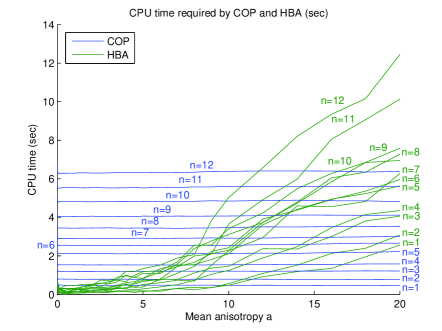
(a)

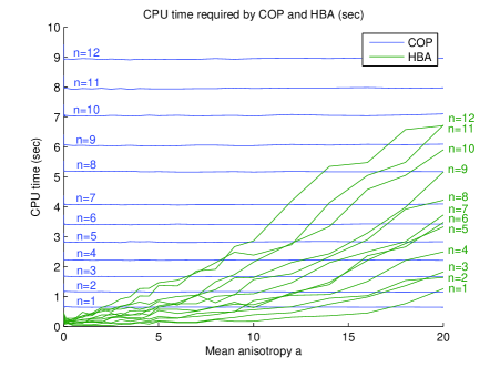
(b)

Figure 1: Mean CPU time required to compute the $a$-anisotropic norm by the convex optimization (COP) and homotopy-based algorithm (HBA); $n=\{1\ldots 12\}$, $p=2$, $m=3$ (a), $m=5$ (b).

At the same time, the average values in Tables 1, 2 do not take into account the growth of the mean CPU time required by HBA over all realizations of equal dimensions as the mean anisotropy level $a$ increases. This growth is clearly demonstrated by the diagrams in Figure 1, where the mean CPU time is shown as a function of the mean anisotropy level $a$ for all groups of realizations of equal dimensions. These diagrams also show that the mean CPU time required by COP does not change noticeably with the increase of $a$.

The data in Tables 3, 4 are concerned with the reliability of the algorithms being compared. The percentages of successful and failed runs, infeasible problems, as well as runs with numerical problems (COP) including the maximum admissible number of iterations (HBA) exceeded were calculated as the average value over all realizations of equal dimensions and over the set of 27 different values of the input mean anisotropy level $a\in[0,20]$. The analysis of Tables 3, 4 shows that computation of the $a$-anisotropic norm from the solution to COP have more successful runs than HBA on average. Moreover, all failed runs of the optimization-based algorithm are caused by infeasibility of the respective COP. Their fraction corresponds to the percentage of realizations with poles located very close to the unit circle in the total number of tested realizations. It should be noted that HBA had the same percentage of runs failed because of the infeasibility of algebraic Riccati equation. However, this algorithm is also characterized by a certain percentage of runs with the maximum number of iterations exceeded and runs which resulted in unexpected crashes in the Lyapunov and Riccati equation solvers.

Table 3: Successful and failed runs; $n=1\ldots 12,$ $m=3$, $p=2$

	COP				HBA
	Succ.	Failed	Infeas.	Numer.	Succ.	Failed	Infeas.	Max. iter.
$n$	(%)	(%)	(%)	probl. (%)	(%)	(%)	(%)	exceed. (%)
1	100	0	0	5.1538	85.5385	14.4615	0	9.0385
2	99	1	1	4.0385	81.6923	18.3077	1	10.4231
3	90.1154	9.8846	9.8846	5.1154	70.3462	29.6538	9.8846	12.7308
4	95.5769	4.4231	4.4231	7.0385	75.2692	24.7308	4.4231	11.5769
5	92	8	8	9.2692	70.2308	29.7692	8	12.3462
6	91	9	9	12.2692	66.8846	33.1154	9	15.3846
7	94.7692	5.2308	5.2308	16.0769	68.0769	31.9231	5.2308	14.3077
8	88.1154	11.8846	11.8846	15.8077	67.6154	32.3846	11.8846	13.7692
9	92.3846	7.6154	7.6154	18.3846	63.5385	36.4615	7.6154	16.5000
10	88.4231	11.5769	11.5769	21.5000	62.8846	37.1154	11.5769	13.5000
11	89.8462	10.1538	10.1538	21.1154	65.7692	34.2308	10.1538	12.6923
12	91.4231	8.5769	8.5769	26.3077	66.4231	33.5769	8.5769	16

Table 4: Successful and failed runs; $n=1\ldots 12,$ $m=5$, $p=2$

	COP				HBA
	Succ.	Failed	Infeas.	Numer.	Succ.	Failed	Infeas.	Max. iter.
$n$	(%)	(%)	(%)	probl. (%)	(%)	(%)	(%)	exceed. (%)
1	100	0	0	4.1154	92.0769	7.9231	0	3.6923
2	97	3	3	3.7308	87.1538	12.8462	3	5.0769
3	93	7	7	3.6923	82.1154	17.8846	7	6.0769
4	95.8462	4.1538	4.1538	4.4615	82.9231	17.0769	4.1538	7.9615
5	92.6923	7.3077	7.3077	4.6154	77.4615	22.5385	7.3077	9.6923
6	97.7308	2.2692	2.2692	4.8846	80.7308	19.2692	2.2692	8.2692
7	87.3846	12.6154	12.6154	5.1538	69.6154	30.3846	12.6154	10.6538
8	89.9615	10.0385	10.0385	4.5000	77.9615	22.0385	10.0385	9.9615
9	88.3462	11.6538	11.6538	5.4615	70.9231	29.0769	11.6538	10.5769
10	92.7308	7.2692	7.2692	5.9231	74.8462	25.1538	7.2692	12.2692
11	86.5769	13.4231	13.4231	6.9615	67.6538	32.3462	13.4231	12.6538
12	91.3077	8.6923	8.6923	7.9231	70.2692	29.7308	8.6923	14.3846

Finally, Table 5 gathers together the mean CPU time required and percentages of successful and failed runs computed as average values over all realizations irrespective of dimensions for different values of the input mean anisotropy level $a\in[0,20]$. It can be seen that the mean CPU time required by HBA grows with increase of $a$. The same is true in regard to the percentage of the HBA runs failed by the maximum number of iterations exceeded. The percentage of HBA successful runs decreases considerably as $a$ increases. At the same time, the mean CPU time required by COP and the percentage of successful runs of this algorithm change insignificantly with the growth of the input mean anisotropy level.

Table 5: Mean CPU time required, successful and failed runs for different values of $a$; all tested realizations

	COP				HBA
	Mean CPU	Succ.	Infeas.	Numer.	Mean CPU	Succ.	Infeas.	Max. iter.
$a$	time (s)	(%)	(%)	probl. (%)	time (s)	(%)	(%)	exceed. (%)
0	3.9341	93.2083	6.7917	14.5417	—	0	—	0
0.02	3.6000	93.2083	6.7917	6.7917	0.2864	88.7083	6.7917	2.3333
0.04	3.6098	93.2083	6.7917	6.7917	0.2400	89.8333	6.7917	1.7500
0.06	3.6273	93.1667	6.8333	6.8333	0.2261	90.4167	6.8333	1.6250
0.08	3.6282	93.1667	6.8333	6.8333	0.2113	90.7500	6.8333	1.4167
0.1	3.6246	93.1667	6.8333	6.8333	0.1893	91.0417	6.8333	1.1250
0.5	3.6184	93.1667	6.8333	6.8750	0.1615	92.2083	6.8333	0.6667
1	3.6185	93.1667	6.8333	7.0417	0.2184	91.3333	6.8333	1.5833
1.5	3.6175	93.0417	6.9583	7.1667	0.2509	90.9167	6.9583	2.0000
2	3.6189	93.0000	7.0000	7.2500	0.3209	89.8333	7.0000	3.0417
2.5	3.6195	92.9167	7.0833	7.3750	0.3574	89.3750	7.0833	3.4583
3	3.6179	92.8750	7.1250	7.4167	0.3926	88.7917	7.1250	3.9167
3.5	3.6163	92.8333	7.1667	7.4583	0.4593	87.8750	7.1667	4.7917
4	3.6196	92.7917	7.2083	7.5417	0.5338	86.7500	7.2083	5.7917
4.5	3.6206	92.7917	7.2083	7.6250	0.5498	86.3750	7.2083	6.0000
5	3.6197	92.7083	7.2917	7.7083	0.6754	84.3333	7.2917	7.6667
6	3.6213	92.5000	7.5000	8.0833	0.7531	83.1250	7.5000	8.4167
7	3.6201	92.3750	7.6250	8.3750	0.9554	79.9167	7.6250	10.7500
8	3.6265	92.2083	7.7917	8.8333	1.1690	76.5417	7.7917	13.0417
9	3.6308	92.1250	7.8750	9.3333	1.4899	72.0000	7.8750	16.3333
10	3.6307	92.1250	7.8750	9.8750	1.7947	68.0417	7.8750	19.7083
12	3.6445	92.1667	7.8333	10.6250	2.4873	58.7500	7.8333	27.4167
14	3.6441	92.2917	7.7083	11.2917	3.1595	49.3750	7.7083	33.6250
16	3.6492	92.1250	7.8750	12.2083	3.8370	40.5000	7.8750	37.5833
18	3.6517	92.0417	7.9583	12.7917	4.4236	32.8750	7.9583	39.6667
20	3.6545	92.2917	7.7083	12.9167	5.1172	26.5000	7.7083	38.2917

5 Conclusion

We have introduced the Strict Anisotropic Norm Bounded Real Lemma in terms of inequalities providing a state-space criterion for verifying if the anisotropic norm of a LDTI system is bounded by a given threshold value. This result extends the ${\mathcal{H}_{\infty}}$ Bounded Real Lemma to stochastic systems where the statistical uncertainty, present in the random disturbances, is quantified by the mean anisotropy level.

The derived criterion employs the solution of an LMI and an inequality on the determinant of a related positive definite matrix and a positive scalar parameter. SANBRL in terms of inequalities provides a key result which is used for the design of suboptimal (or $\gamma$-optimal) anisotropic controllers via convex optimization and semidefinite programming to ensure a specified upper bound on the anisotropic norm of the closed-loop system (respectively, to minimize the norm). It can also be combined with additional specifications for the controllers.

References

- [1] A.V. Semyonov, I.G. Vladimirov, and A.P. Kurdjukov. Stochastic approach to -optimization. Proc. 33rd IEEE Conf. on Decision and Control, Florida, USA, 1994, pages 2249–2250.
- [2] I.G. Vladimirov, A.P. Kurdjukov, and A.V. Semyonov. Anisotropy of signals and the entropy of linear stationary systems. Doklady Math., 51:388–390, 1995.
- [3] I.G. Vladimirov, A.P. Kurdjukov, and A.V. Semyonov. On computing the anisotropic norm of linear discrete-time-invariant systems. Proc. 13th IFAC World Congress, San-Francisco, CA, pages 179–184, 1996.
- [4] I.G. Vladimirov, A.P. Kurdjukov, and A.V. Semyonov. State-space solution to anisotropy-based stochastic -optimization problem. Proc. 13th IFAC World Congress, San Francisco, CA, pages 427–432, 1996.
- [5] P. Diamond, A.P. Kurdjukov, A.V. Semyonov, and I.G. Vladimirov. Homotopy methods and anisotropy-based stochastic optimization of control systems. Report 97-14 of The University of Queensland, Australia, pages 1–22, 1997.
- [6] A.P. Kurdyukov, E.A. Maximov, and M.M. Tchaikovsky. Anisotropy-based bounded real lemma. Proc. 19th International Symposium on Mathematical Theory of Networks and Systems, Budapest, Hungary, pages 2391–2397, 2010.
- [7] E.A. Maximov, A.P. Kurdyukov, and I.G. Vladimirov. Anisotropy-based bounded real lemma for linear discrete time varying systems. Proc. 18th IFAC World Congress, Milano, Italy, 2011.
- [8] M.M. Tchaikovsky, A.P. Kurdyukov, and V.N. Timin. Synthesis of anisotropic suboptimal controllers by convex optimization. Preprint. Available from http://arxiv.org/abs/1108.4982, 2011.
- [9] P. Diamond, I.G. Vladimirov, A.P. Kurdyukov, and A.V. Semyonov. Anisotropy-based performance analysis of linear discrete time invariant control systems. Int. J. of Contr., 74:28–42, 2001.
- [10] I.G. Vladimirov, P. Diamond, and P. Kloeden. Anisotropy-based performance analysis of finite horizon linear discrete time varying systems. Automat. & and Remote Contr., 8:1265–1282, 2006.
- [11] T.M. Cover and J.A. Thomas. Elements of Information Theory. John Wiley and Sons, 1991.
- [12] Yu. Nesterov and A. Nemirovskii. Interior-Point Polynomial Methods in Convex Programming, volume 13 of Studies in Applied Mathematics. SIAM, Philadelphia, PA, 1994.
- [13] A. Ben-Tal and A. Nemirovskii. Lectures on Modern Convex Optimization. Technion, Haifa, Israel, 2000.
- [14] C.E. de Souza and L. Xie. On the discrete-time bounded real lemma with application in the characterization of static state feedback controllers. Syst. Contr. Let., 18:61–71, 1992.
- [15] C.E. de Souza. On stabilizing properties of solutions of the Riccati difference equation. IEEE Trans. AC, AC-34:1313–1316, 1989.
- [16] D.S. Bernstein. Matrix Mathematics: Theory, Facts, and Formulas with Application to Linear Systems Theory. Princeton University Press, Princeton, NJ, 2005.
- [17] A.S. Poznyak. Advanced Mathematical Tools for Automatic Control Engineers. Volumes 1,2: Deterministic Techniques, Stochastic Techniques. Elsevier, 2008, 2009.
- [18] P. Gahinet and P. Apkarian. A linear matrix inequality approach to control. Int. J. of Robust and Nonlinear Contr., 4:421–448, 1994.
- [19] J. Löfberg. YALMIP: A toolbox for modeling and optimization in MATLAB. Proc. of the CACSD Conference, Taipei, Taiwan, 2004. Available from control.ee.ethz.ch/joloef/wiki/pmwiki.php.
- [20] J.F. Sturm. Using SeDuMi 1.02, a MATLAB toolbox for optimization over symmetric cones. Optimization Methods and Software, 11:625–653, 1999.