\addtokomafont

disposition

B𝐵B-decay CP-asymmetries in SUSY
with a U(2)3𝑈superscript23U(2)^{3} flavour symmetry

Riccardo Barbieria    Paolo Camplia    Gino Isidorib   
Filippo Salaa and David M. Strauba
a
Scuola Normale Superiore and INFN, Piazza dei Cavalieri 7, 56126 Pisa, Italy
bINFN, Laboratori Nazionali di Frascati, Via E. Fermi 40, 00044 Frascati, Italy
Abstract

We study CP asymmetries in rare B𝐵B decays within supersymmetry with a U(2)3𝑈superscript23U(2)^{3} flavour symmetry, motivated by the SUSY flavour and CP problems, the hierarchies in the Yukawa couplings and the absence so far of any direct evidence for SUSY. Even in the absence of flavour-blind phases, we find potentially sizable CP violating contributions to bs𝑏𝑠b\to s decay amplitudes. The effects in the mixing-induced CP asymmetries in BϕKS𝐵italic-ϕsubscript𝐾𝑆B\to\phi K_{S} and BηKS𝐵superscript𝜂subscript𝐾𝑆B\to\eta^{\prime}K_{S}, angular CP asymmetries in BKμ+μ𝐵superscript𝐾superscript𝜇superscript𝜇B\to K^{*}\mu^{+}\mu^{-} and the direct CP asymmetry in BXsγ𝐵subscript𝑋𝑠𝛾B\to X_{s}\gamma can be in the region to be probed by LHCb and next generation B𝐵B factories. At the same time, these effects in B decays are compatible with CP violating contributions to meson mixing, including a non-standard Bssubscript𝐵𝑠B_{s} mixing phase hinted by current tensions in the CKM fit mostly between SψKS,ϵKsubscript𝑆𝜓subscript𝐾𝑆subscriptitalic-ϵ𝐾S_{\psi K_{S}},\epsilon_{K} and ΔMBs/ΔMBdΔsubscript𝑀subscript𝐵𝑠Δsubscript𝑀subscript𝐵𝑑\Delta M_{B_{s}}/\Delta M_{B_{d}}.

1 Introduction

Weak scale supersymmetry has long been the leading candidate for physics beyond the Standard Model (SM), but it is increasingly challenged by the lack of any clear experimental evidence in its favour. Arguably, the most important challenges to be explained are the success of the CKM description of flavour violation, the tight bounds on flavour-blind CP violation from electric dipole moment (EDM) searches and the tightening sparticle mass bounds from LHC.

A promising approach to address these three problems is to make use of the fact that the third generation of quarks is special, since it has sizable Yukawa couplings and is weakly mixed with the first two generations. If the first two generations of quarks and squarks form doublets under a U(2)𝑈2U(2) flavour symmetry commuting with the gauge group, the flavour problem is ameliorated while at the same time the hierarchies in the Yukawa couplings can be (at least partially) understood [1, 2]. Furthermore, a flavour symmetry for the light quark generations fits well to a hierarchy in the spectrum of squarks, with the third generation partners being light and the first two generation ones in the multi-TeV region [3, 4, 5, 6]. This has two virtues, in addition to further ameliorating the flavour problem: First, it solves the CP problem, decoupling the contributions of flavour-blind phases to the observable EDMs, which involve first generation fermions [7]. Second, it evades the strongest sparticle direct search bounds. While the lower bounds on first two generation squark masses from LHC are approaching a TeV, third generation squarks can still be in the few-hundred GeV region for gluino masses above about 600600600 GeV, depending on the gluino decay branching ratios and on the lightest neutralino mass.111For a first LHC analysis with about 1fb11superscriptfb11~{}\text{fb}^{-1} of integrated luminosity, see [8, 9].

Motivated by these facts, a U(2)3𝑈superscript23U(2)^{3} symmetry has been considered in [10] together with a hierarchical squark spectrum and has been shown to solve, in addition to the above-mentioned problems, tensions present in the fits of the CKM matrix by contributing to CP violation in meson mixing. In this way, a non-standard Bssubscript𝐵𝑠B_{s} mixing phase was predicted, as currently hinted by Tevatron data [11, 12].

The purpose of this article is to extend the analysis in [10] to ΔF=1Δ𝐹1\Delta F=1 processes, i.e. rare decays, studying in particular possible signatures of CP violation correlated with the predicted CP violation in meson mixing (ΔF=2Δ𝐹2\Delta F=2). Contrary to the ΔF=2Δ𝐹2\Delta F=2 sector, where the pattern of deviations from the SM identified in [10] is unambiguously dictated by the U(2)3𝑈superscript23U(2)^{3} symmetry, the predictions of ΔF=1Δ𝐹1\Delta F=1 observables are more model dependent. In this analysis we concentrate on a framework with moderate values of tanβ𝛽\tan\beta and, in order to establish a link between ΔF=2Δ𝐹2\Delta F=2 and ΔF=1Δ𝐹1\Delta F=1 CP-violating observables, we take small flavour-blind phases and assume the dominance of gluino-mediated flavour-changing amplitudes.

2 Setup

We briefly review the U(2)3𝑈superscript23U(2)^{3} framework, referring to [10] for details and derivations. We consider a global flavour symmetry

GF=U(2)Q×U(2)u×U(2)dsubscript𝐺𝐹𝑈subscript2𝑄𝑈subscript2𝑢𝑈subscript2𝑑G_{F}=U(2)_{Q}\times U(2)_{u}\times U(2)_{d} (1)

broken minimally by three spurions, transforming as ΔYu=(2,2¯,1)Δsubscript𝑌𝑢2¯21\Delta Y_{u}=(2,\bar{2},1), ΔYd=(2,1,2¯)Δsubscript𝑌𝑑21¯2\Delta Y_{d}=(2,1,\bar{2}) and V=(2,1,1)𝑉211V=(2,1,1), respectively. This breaking pattern leads to non-minimal flavour violation in the down quark-squark-gluino vertex,

(d¯L,RWL,Rdd~L,R)g~.subscript¯𝑑𝐿𝑅subscriptsuperscript𝑊𝑑𝐿𝑅subscript~𝑑𝐿𝑅~𝑔(\bar{d}_{L,R}W^{d}_{L,R}\tilde{d}_{L,R})\tilde{g}. (2)

which can be approximately written as

WLd=(cdκκsLeiγLκcdcdsLeiγL0sLeiγL1),WRd=𝟙,formulae-sequencesubscriptsuperscript𝑊𝑑𝐿subscript𝑐𝑑superscript𝜅superscript𝜅subscript𝑠𝐿superscript𝑒𝑖subscript𝛾𝐿𝜅subscript𝑐𝑑subscript𝑐𝑑subscript𝑠𝐿superscript𝑒𝑖subscript𝛾𝐿0subscript𝑠𝐿superscript𝑒𝑖subscript𝛾𝐿1subscriptsuperscript𝑊𝑑𝑅1W^{d}_{L}=\left(\begin{array}[]{ccc}c_{d}&\kappa^{*}&-\kappa^{*}s_{L}e^{i\gamma_{L}}\\ -\kappa&c_{d}&-c_{d}s_{L}e^{i\gamma_{L}}\\ 0&s_{L}e^{-i\gamma_{L}}&1\\ \end{array}\right),\qquad W^{d}_{R}=\mathbbm{1}\,, (3)

where κ=cdVtd/Vts𝜅subscript𝑐𝑑subscript𝑉𝑡𝑑subscript𝑉𝑡𝑠\kappa=c_{d}V_{td}/V_{ts} and cdsubscript𝑐𝑑c_{d} is fixed by the CKM matrix, which in these conventions reads

VCKM=(1λ2/2λsuseiδλ1λ2/2cussdsei(ϕ+δ)scd1),subscript𝑉CKM1superscript𝜆22𝜆subscript𝑠𝑢𝑠superscript𝑒𝑖𝛿𝜆1superscript𝜆22subscript𝑐𝑢𝑠subscript𝑠𝑑𝑠superscript𝑒𝑖italic-ϕ𝛿𝑠subscript𝑐𝑑1V_{\text{CKM}}=\left(\begin{array}[]{ccc}1-\lambda^{2}/2&\lambda&s_{u}se^{-i\delta}\\ -\lambda&1-\lambda^{2}/2&c_{u}s\\ -s_{d}s\,e^{i(\phi+\delta)}&-sc_{d}&1\\ \end{array}\right), (4)

where sucdcusdeiϕ=λeiδsubscript𝑠𝑢subscript𝑐𝑑subscript𝑐𝑢subscript𝑠𝑑superscript𝑒𝑖italic-ϕ𝜆superscript𝑒𝑖𝛿s_{u}c_{d}-c_{u}s_{d}e^{-i\phi}=\lambda e^{i\delta}. A direct fit of this parametrization to tree-level observables results in

susubscript𝑠𝑢\displaystyle s_{u} =0.086±0.003,absentplus-or-minus0.0860.003\displaystyle=0.086\pm 0.003\,, sdsubscript𝑠𝑑\displaystyle s_{d} =0.22±0.01,absentplus-or-minus0.220.01\displaystyle=-0.22\pm 0.01\,, (5)
s𝑠\displaystyle s =0.0411±0.0005,absentplus-or-minus0.04110.0005\displaystyle=0.0411\pm 0.0005\,, ϕitalic-ϕ\displaystyle\phi =(97±9).absentsuperscriptplus-or-minus979\displaystyle=(-97\pm 9)^{\circ}\,. (6)

The mixing sLsubscript𝑠𝐿s_{L} and the phase222Our phase γLsubscript𝛾𝐿\gamma_{L} is equivalent to the phase γ𝛾\gamma in [10]. γLsubscript𝛾𝐿\gamma_{L} in (3), on the other hand, are free parameters. Defining

ξL=cdsL|Vts|eiγL,subscript𝜉𝐿subscript𝑐𝑑subscript𝑠𝐿subscript𝑉𝑡𝑠superscript𝑒𝑖subscript𝛾𝐿\xi_{L}=\dfrac{c_{d}s_{L}}{|V_{ts}|}e^{i\gamma_{L}}\,, (7)

the mixing amplitudes in the K𝐾K, Bdsubscript𝐵𝑑B_{d} and Bssubscript𝐵𝑠B_{s} meson systems are modified as follows,

M12Ksuperscriptsubscript𝑀12𝐾\displaystyle M_{12}^{K} =(M12K)SM(tt)(1+|ξL|4F0)+(M12K)SM(tc+cc),absentsuperscriptsubscriptsuperscriptsubscript𝑀12𝐾SM𝑡𝑡1superscriptsubscript𝜉𝐿4subscript𝐹0superscriptsubscriptsuperscriptsubscript𝑀12𝐾SM𝑡𝑐𝑐𝑐\displaystyle=\left(M_{12}^{K}\right)_{\text{SM}}^{(tt)}\left(1+|\xi_{L}|^{4}F_{0}\right)+\left(M_{12}^{K}\right)_{\text{SM}}^{(tc+cc)}, (8)
M12Bd,ssuperscriptsubscript𝑀12subscript𝐵𝑑𝑠\displaystyle M_{12}^{B_{d,s}} =(M12Bd,s)SM(1+ξL2F0),absentsubscriptsuperscriptsubscript𝑀12subscript𝐵𝑑𝑠SM1superscriptsubscript𝜉𝐿2subscript𝐹0\displaystyle=\left(M_{12}^{B_{d,s}}\right)_{\text{SM}}\left(1+\xi_{L}^{2}F_{0}\right), (9)

where F0>0subscript𝐹00F_{0}>0 is a loop function, predicting a universal shift in the Bdsubscript𝐵𝑑B_{d} and Bssubscript𝐵𝑠B_{s} mixing phases. The mixing induced CP asymmetries in BψKS𝐵𝜓subscript𝐾𝑆B\to\psi K_{S} and Bsψϕsubscript𝐵𝑠𝜓italic-ϕB_{s}\to\psi\phi are thus

SψKS=sin(2β+ϕΔ),Sψϕ=sin(2|βs|ϕΔ),formulae-sequencesubscript𝑆𝜓subscript𝐾𝑆2𝛽subscriptitalic-ϕΔsubscript𝑆𝜓italic-ϕ2subscript𝛽𝑠subscriptitalic-ϕΔS_{\psi K_{S}}=\sin\left(2\beta+\phi_{\Delta}\right)\,,\qquad S_{\psi\phi}=\sin\left(2|\beta_{s}|-\phi_{\Delta}\right)\,, (10)

where ϕΔ=arg(1+ξL2F0)subscriptitalic-ϕΔarg1superscriptsubscript𝜉𝐿2subscript𝐹0\phi_{\Delta}=\text{arg}\!\left(1+\xi_{L}^{2}F_{0}\right).

The current tensions in the CKM fit arising mostly between SψKSsubscript𝑆𝜓subscript𝐾𝑆S_{\psi K_{S}}, |ϵK|subscriptitalic-ϵ𝐾|\epsilon_{K}| and ΔMs/ΔMdΔsubscript𝑀𝑠Δsubscript𝑀𝑑\Delta M_{s}/\Delta M_{d} can be accommodated by the shifts in SψKSsubscript𝑆𝜓subscript𝐾𝑆S_{\psi K_{S}} and |ϵK|subscriptitalic-ϵ𝐾|\epsilon_{K}|. Assuming this to be the case, a global fit of the CKM matrix to ΔF=2Δ𝐹2\Delta F=2 observables including the supersymmetric contributions leads to the following predictions at the 90%percent9090\% C.L.,

0.8<|ξL|<2.1,0.8subscript𝜉𝐿2.1\displaystyle 0.8<|\xi_{L}|<2.1\,, (11)
9<ϕΔ<1,superscript9subscriptitalic-ϕΔsuperscript1\displaystyle-9^{\circ}<\phi_{\Delta}<-1^{\circ}\,, (12)
86<γL<25 or 94<γL<155,superscript86subscript𝛾𝐿superscript25 or superscript94subscript𝛾𝐿superscript155\displaystyle-86^{\circ}<\gamma_{L}<-25^{\circ}\text{ ~{}or~{} }94^{\circ}<\gamma_{L}<155^{\circ}\,, (13)
0.05<Sψϕ<0.20,.0.05subscript𝑆𝜓italic-ϕ0.20\displaystyle 0.05<S_{\psi\phi}<0.20,\,. (14)

with gluino and left-handed sbottom masses necessarily below 1÷1.511.51\div 1.5 TeV. The ambiguity in γLsubscript𝛾𝐿\gamma_{L} stems from the fact that the ΔF=2Δ𝐹2\Delta F=2 observables are only sensitive to the phase of ξL2superscriptsubscript𝜉𝐿2\xi_{L}^{2}, and thus to 2γL2subscript𝛾𝐿2\gamma_{L}.

The presence of the phase γLsubscript𝛾𝐿\gamma_{L} leads to contributions to CP asymmetries in B𝐵B physics. Additional contributions can arise from flavour-blind phases, such as the phase of the μ𝜇\mu term or the trilinear couplings. With hierarchical sfermions, such phases are not required to be small to meet the EDM constraints [7]. Still, to concentrate on the genuine U(2)3𝑈superscript23U(2)^{3} effects, we will take flavour blind phases to be absent in the following and thus focus on B𝐵B physics.

3 ΔB=1Δ𝐵1\Delta B=1 effective Hamiltonian

The part of the bs𝑏𝑠b\to s effective Hamiltonian sensitive to NP in our setup reads

effsubscripteff\displaystyle\mathcal{H}_{\text{eff}} =4GF2VtsVtbi=310CiOi+ h.c.,absent4subscript𝐺𝐹2superscriptsubscript𝑉𝑡𝑠subscript𝑉𝑡𝑏superscriptsubscript𝑖310subscript𝐶𝑖subscript𝑂𝑖 h.c.\displaystyle=\frac{4G_{F}}{\sqrt{2}}V_{ts}^{*}V_{tb}\sum_{i=3}^{10}C_{i}O_{i}+\text{ h.c.}\,, (15)
O3subscript𝑂3\displaystyle O_{3} =(s¯PLb)q(q¯PLq)absent¯𝑠subscript𝑃𝐿𝑏subscript𝑞¯𝑞subscript𝑃𝐿𝑞\displaystyle=(\bar{s}P_{L}b){\textstyle\sum}_{q}(\bar{q}P_{L}q)\qquad O4subscript𝑂4\displaystyle O_{4} =(s¯αPLbβ)q(qβ¯PLqα)absentsubscript¯𝑠𝛼subscript𝑃𝐿subscript𝑏𝛽subscript𝑞¯subscript𝑞𝛽subscript𝑃𝐿subscript𝑞𝛼\displaystyle=(\bar{s}_{\alpha}P_{L}b_{\beta}){\textstyle\sum}_{q}(\bar{q_{\beta}}P_{L}q_{\alpha})
O5subscript𝑂5\displaystyle O_{5} =(s¯PLb)q(q¯PRq)absent¯𝑠subscript𝑃𝐿𝑏subscript𝑞¯𝑞subscript𝑃𝑅𝑞\displaystyle=(\bar{s}P_{L}b){\textstyle\sum}_{q}(\bar{q}P_{R}q)\qquad O6subscript𝑂6\displaystyle O_{6} =(s¯αPLbβ)q(qβ¯PRqα)absentsubscript¯𝑠𝛼subscript𝑃𝐿subscript𝑏𝛽subscript𝑞¯subscript𝑞𝛽subscript𝑃𝑅subscript𝑞𝛼\displaystyle=(\bar{s}_{\alpha}P_{L}b_{\beta}){\textstyle\sum}_{q}(\bar{q_{\beta}}P_{R}q_{\alpha})
O7subscript𝑂7\displaystyle O_{7} =e16π2mb(s¯σμνPRb)Fμνabsent𝑒16superscript𝜋2subscript𝑚𝑏¯𝑠subscript𝜎𝜇𝜈subscript𝑃𝑅𝑏subscript𝐹𝜇𝜈\displaystyle=\frac{e}{16\pi^{2}}m_{b}(\bar{s}\sigma_{\mu\nu}P_{R}b)F_{\mu\nu}\qquad O8subscript𝑂8\displaystyle O_{8} =gs16π2mb(s¯σμνPRb)Gμνabsentsubscript𝑔𝑠16superscript𝜋2subscript𝑚𝑏¯𝑠subscript𝜎𝜇𝜈subscript𝑃𝑅𝑏subscript𝐺𝜇𝜈\displaystyle=\frac{g_{s}}{16\pi^{2}}m_{b}(\bar{s}\sigma_{\mu\nu}P_{R}b)G_{\mu\nu}
O9subscript𝑂9\displaystyle O_{9} =e216π2(s¯γμPLb)(l¯γμl)absentsuperscript𝑒216superscript𝜋2¯𝑠subscript𝛾𝜇subscript𝑃𝐿𝑏¯𝑙subscript𝛾𝜇𝑙\displaystyle=\frac{e^{2}}{16\pi^{2}}(\bar{s}\gamma_{\mu}P_{L}b)(\bar{l}\gamma_{\mu}l)\qquad O10subscript𝑂10\displaystyle O_{10} =e216π2(s¯γμPLb)(l¯γμγ5l)absentsuperscript𝑒216superscript𝜋2¯𝑠subscript𝛾𝜇subscript𝑃𝐿𝑏¯𝑙subscript𝛾𝜇subscript𝛾5𝑙\displaystyle=\frac{e^{2}}{16\pi^{2}}(\bar{s}\gamma_{\mu}P_{L}b)(\bar{l}\gamma_{\mu}\gamma_{5}l)

The QCD penguin operators O36subscript𝑂36O_{3\ldots 6} are relevant for the CP asymmetries in bss¯s𝑏𝑠¯𝑠𝑠b\to s\bar{s}s penguin decays to be discussed below. In the case of hierarchical sfermions, the box contributions are mass-suppressed and we only have to consider gluon penguins, which contribute in a universal way as

C3=C5=13C4=13C6CG.subscript𝐶3subscript𝐶513subscript𝐶413subscript𝐶6subscript𝐶𝐺C_{3}=C_{5}=-\tfrac{1}{3}C_{4}=-\tfrac{1}{3}C_{6}\equiv C_{G}\,. (16)

The analogous photon penguin can be neglected in non-leptonic decays since it is suppressed by αem/αssubscript𝛼𝑒𝑚subscript𝛼𝑠\alpha_{em}/\alpha_{s}, but it can contribute to C9subscript𝐶9C_{9}. There is no effect in C10subscript𝐶10C_{10}, which remains SM-like.

In the MSSM, the ΔF=1Δ𝐹1\Delta F=1 effective Hamiltonian receives contributions from loops involving charginos, neutralinos, charged Higgs bosons or gluinos. In the following, we will concentrate for simplicity on gluino contributions, which are always proportional to the complex ξLsubscript𝜉𝐿\xi_{L} in U(2)3𝑈superscript23U(2)^{3}. Among the remaining contributions, some are proportional to ξLsubscript𝜉𝐿\xi_{L} while some are real in the absence of flavour blind phases. Their omission does not qualitatively change our predictions for CP asymmetries, but we stress that the real contributions can have an impact in particular on the branching ratios to be considered below.

The gluino contributions to CGsubscript𝐶𝐺C_{G} and C9subscript𝐶9C_{9} are

CG=ξLαsα2αs4πmW2mb~213108fG(xg~),C9=ξLαsα2mW2mb~2227fγ(xg~),formulae-sequencesubscript𝐶𝐺subscript𝜉𝐿subscript𝛼𝑠subscript𝛼2subscript𝛼𝑠4𝜋superscriptsubscript𝑚𝑊2superscriptsubscript𝑚~𝑏213108subscript𝑓𝐺subscript𝑥~𝑔subscript𝐶9subscript𝜉𝐿subscript𝛼𝑠subscript𝛼2superscriptsubscript𝑚𝑊2superscriptsubscript𝑚~𝑏2227subscript𝑓𝛾subscript𝑥~𝑔C_{G}=-\xi_{L}\;\dfrac{\alpha_{s}}{\alpha_{2}}\;\dfrac{\alpha_{s}}{4\pi}\;\dfrac{m_{W}^{2}}{m_{\tilde{b}}^{2}}\;\dfrac{13}{108}f_{G}(x_{\tilde{g}})\,,\qquad C_{9}=\xi_{L}\;\dfrac{\alpha_{s}}{\alpha_{2}}\;\dfrac{m_{W}^{2}}{m_{\tilde{b}}^{2}}\;\dfrac{2}{27}f_{\gamma}(x_{\tilde{g}})\,, (17)

where here and throughout, xg~=mg~2/mb~2subscript𝑥~𝑔superscriptsubscript𝑚~𝑔2superscriptsubscript𝑚~𝑏2x_{\tilde{g}}=m_{\tilde{g}}^{2}/m_{\tilde{b}}^{2} and all the loop functions are defined such that fi(1)=1subscript𝑓𝑖11f_{i}(1)=1 with the exact form given in appendix A.

The main difference concerning the magnetic and chromomagnetic Wilson coefficients C7subscript𝐶7C_{7} and C8subscript𝐶8C_{8} is that here b~Lsubscript~𝑏𝐿\tilde{b}_{L}-b~Rsubscript~𝑏𝑅\tilde{b}_{R} mass insertion contributions are important, while for the other Wilson coefficients they were chirality-suppressed. The gluino contributions read

C7subscript𝐶7\displaystyle C_{7} =ξLαsα2mW2mb~2127[f7(xg~)+2μtanβAbmg~g7(xg~)],absentsubscript𝜉𝐿subscript𝛼𝑠subscript𝛼2superscriptsubscript𝑚𝑊2superscriptsubscript𝑚~𝑏2127delimited-[]subscript𝑓7subscript𝑥~𝑔2𝜇𝛽subscript𝐴𝑏subscript𝑚~𝑔subscript𝑔7subscript𝑥~𝑔\displaystyle=-\xi_{L}\;\dfrac{\alpha_{s}}{\alpha_{2}}\;\dfrac{m_{W}^{2}}{m_{\tilde{b}}^{2}}\;\dfrac{1}{27}\left[f_{7}(x_{\tilde{g}})+2\dfrac{\mu\tan\beta-A_{b}}{m_{\tilde{g}}}g_{7}(x_{\tilde{g}})\right]\,, (18)
C8subscript𝐶8\displaystyle C_{8} =ξLαsα2mW2mb~2536[f8(xg~)+2μtanβAbmg~g8(xg~)].absentsubscript𝜉𝐿subscript𝛼𝑠subscript𝛼2superscriptsubscript𝑚𝑊2superscriptsubscript𝑚~𝑏2536delimited-[]subscript𝑓8subscript𝑥~𝑔2𝜇𝛽subscript𝐴𝑏subscript𝑚~𝑔subscript𝑔8subscript𝑥~𝑔\displaystyle=-\xi_{L}\;\dfrac{\alpha_{s}}{\alpha_{2}}\;\dfrac{m_{W}^{2}}{m_{\tilde{b}}^{2}}\;\dfrac{5}{36}\left[f_{8}(x_{\tilde{g}})+2\dfrac{\mu\tan\beta-A_{b}}{m_{\tilde{g}}}g_{8}(x_{\tilde{g}})\right]\,. (19)

For mg~=mb~m~subscript𝑚~𝑔subscript𝑚~𝑏~𝑚m_{\tilde{g}}=m_{\tilde{b}}\equiv\tilde{m}, we thus find at the scale mWsubscript𝑚𝑊m_{W}

CGsubscript𝐶𝐺\displaystyle C_{G} =1.1×10⁴(500GeVm~)2ξL,absent1.1superscript104superscript500GeV~𝑚2subscript𝜉𝐿\displaystyle=-1.1\times 10^{-4}\left(\dfrac{500\,{\rm GeV}}{\tilde{m}}\right)^{2}\xi_{L}\,, (20)
Cγsubscript𝐶𝛾\displaystyle C_{\gamma} =9×10³(500GeVm~)2ξL,absent9superscript103superscript500GeV~𝑚2subscript𝜉𝐿\displaystyle=9\times 10^{-3}\left(\dfrac{500\,{\rm GeV}}{\tilde{m}}\right)^{2}\xi_{L}\,, (21)
C7subscript𝐶7\displaystyle C_{7} =3.4×10³(500GeVm~)2ξL[1+2μtanβAbm~],absent3.4superscript103superscript500GeV~𝑚2subscript𝜉𝐿delimited-[]12𝜇𝛽subscript𝐴𝑏~𝑚\displaystyle=-3.4\times 10^{-3}\left(\dfrac{500\,{\rm GeV}}{\tilde{m}}\right)^{2}\xi_{L}\left[1+2\dfrac{\mu\tan\beta-A_{b}}{\tilde{m}}\right], (22)
C8subscript𝐶8\displaystyle C_{8} =1.3×10²(500GeVm~)2ξL[1+2μtanβAbm~].absent1.3superscript102superscript500GeV~𝑚2subscript𝜉𝐿delimited-[]12𝜇𝛽subscript𝐴𝑏~𝑚\displaystyle=-1.3\times 10^{-2}\left(\dfrac{500\,{\rm GeV}}{\tilde{m}}\right)^{2}\xi_{L}\left[1+2\dfrac{\mu\tan\beta-A_{b}}{\tilde{m}}\right]. (23)

A model-independent consequence of the U(2)3𝑈superscript23U(2)^{3} symmetry is that the modification of bs𝑏𝑠b\to s and bd𝑏𝑑b\to d ΔF=1Δ𝐹1\Delta F=1 amplitudes is universal, i.e. only distinguished by the same CKM factors as in the SM (exactly as in the U(3)3𝑈superscript33U(3)^{3}, or MFV case [13]). Therefore, all the expressions for the bs𝑏𝑠b\to s Wilson coefficients derived in this section are also valid for bd𝑏𝑑b\to d processes.

4 B𝐵B physics observables

Observable SM prediction Experiment Future sensitivity
BR(BXsγ)BR𝐵subscript𝑋𝑠𝛾\text{BR}(B\to X_{s}\gamma) (3.15±0.23)×104plus-or-minus3.150.23superscript104(3.15\pm 0.23)\times 10^{-4} [14] (3.52±0.25)×104plus-or-minus3.520.25superscript104(3.52\pm 0.25)\times 10^{-4} ±0.15×10⁴plus-or-minus0.15superscript104\pm 0.15\times 10^{-4}
ACP(bsγ)subscript𝐴CP𝑏𝑠𝛾A_{\text{CP}}(b\to s\gamma) (0.6÷2.8)%percent0.62.8(-0.6\div 2.8)\% [15] (1.2±2.8)%percentplus-or-minus1.22.8(-1.2\pm 2.8)\% ±0.5%plus-or-minuspercent0.5\pm 0.5\%
BR(BXdγ)BR𝐵subscript𝑋𝑑𝛾\text{BR}(B\to X_{d}\gamma) (1.540.31+0.26)×105subscriptsuperscript1.540.260.31superscript105(1.54^{+0.26}_{-0.31})\times 10^{-5} [16] (1.41±0.49)×105plus-or-minus1.410.49superscript105(1.41\pm 0.49)\times 10^{-5}
SϕKSsubscript𝑆italic-ϕsubscript𝐾𝑆S_{\phi K_{S}} 0.68±0.04plus-or-minus0.680.040.68\pm 0.04 [17, 18] 0.560.18+0.16subscriptsuperscript0.560.160.180.56^{+0.16}_{-0.18} ±0.02plus-or-minus0.02\pm 0.02
SηKSsubscript𝑆superscript𝜂subscript𝐾𝑆S_{\eta^{\prime}K_{S}} 0.66±0.03plus-or-minus0.660.030.66\pm 0.03 [17, 18] 0.59±0.07plus-or-minus0.590.070.59\pm 0.07 ±0.01plus-or-minus0.01\pm 0.01
A7delimited-⟨⟩subscript𝐴7\langle A_{7}\rangle (3.4±0.5)×103plus-or-minus3.40.5superscript103(3.4\pm 0.5)\times 10^{-3} [19]
A8delimited-⟨⟩subscript𝐴8\langle A_{8}\rangle (2.6±0.4)×103plus-or-minus2.60.4superscript103(-2.6\pm 0.4)\times 10^{-3} [19]
Table 1: SM predictions, current experimental world averages [20] and experimental sensitivity at planned experiments [21, 22] for the B𝐵B physics observables. <A7,8>expectationsubscript𝐴78<A_{7,8}> are suitable angular CPV asymmetries in BKμ+μ𝐵superscript𝐾superscript𝜇superscript𝜇B\rightarrow K^{*}\mu^{+}\mu^{-}.

4.1 BR(BXqγ𝐵subscript𝑋𝑞𝛾B\to X_{q}\gamma)

The branching ratio of BXsγ𝐵subscript𝑋𝑠𝛾B\to X_{s}\gamma is one of the most important flavour constraints in the MSSM in view of the good agreement between theory and experiment. Experimentally, the quantities

Rbqγ=BR(BXqγ)BR(BXqγ)SMsubscript𝑅𝑏𝑞𝛾BR𝐵subscript𝑋𝑞𝛾BRsubscript𝐵subscript𝑋𝑞𝛾SMR_{bq\gamma}=\frac{\text{BR}({B}\rightarrow X_{q}\gamma)}{\text{BR}({B}\rightarrow X_{q}\gamma)_{\text{SM}}} (24)

are constrained to be

Rbsγ=1.13±0.11,Rbdγ=0.92±0.40,formulae-sequencesubscript𝑅𝑏𝑠𝛾plus-or-minus1.130.11subscript𝑅𝑏𝑑𝛾plus-or-minus0.920.40R_{bs\gamma}=1.13\pm 0.11\,,\qquad R_{bd\gamma}=0.92\pm 0.40\,, (25)

using the numbers in table 1. In U(2)3𝑈superscript23U(2)^{3}, one has RbsγRbdγsubscript𝑅𝑏𝑠𝛾subscript𝑅𝑏𝑑𝛾R_{bs\gamma}\approx R_{bd\gamma} just as in MFV, so the bsγ𝑏𝑠𝛾b\to s\gamma constraint is more important and we will concentrate on it in the following.

Beyond the SM (but in the absence of right-handed currents), the branching ratio can be written as

BR(BXsγ)=R[|C7SM,eff+C7NP,eff|2+N(Eγ)],BR𝐵subscript𝑋𝑠𝛾𝑅delimited-[]superscriptsuperscriptsubscript𝐶7SM,effsuperscriptsubscript𝐶7NP,eff2𝑁subscript𝐸𝛾\text{BR}({B}\rightarrow X_{s}\gamma)=R\left[\left|C_{7}^{\text{SM,eff}}+C_{7}^{\text{NP,eff}}\right|^{2}+N(E_{\gamma})\right], (26)

where R=2.47×10³𝑅2.47superscript103R=2.47\times 10^{-3} and N(Eγ)=(3.6±0.6)×103𝑁subscript𝐸𝛾plus-or-minus3.60.6superscript103N(E_{\gamma})=(3.6\pm 0.6)\times 10^{-3} for a photon energy cut-off Eγ=1.6subscript𝐸𝛾1.6E_{\gamma}=1.6  GeV [23].

Considering only gluino contributions and setting mg~=mb~m~subscript𝑚~𝑔subscript𝑚~𝑏~𝑚m_{\tilde{g}}=m_{\tilde{b}}\equiv\tilde{m}, we find

Rbsγsubscript𝑅𝑏𝑠𝛾\displaystyle R_{bs\gamma} =1+ 2.2×10²(500GeVm~)2|ξL|cosγL(1+2μtanβAbm~).absent12.2superscript102superscript500GeV~𝑚2subscript𝜉𝐿subscript𝛾𝐿12𝜇𝛽subscript𝐴𝑏~𝑚\displaystyle=1\;+\;2.2\times 10^{-2}\left(\dfrac{500\,{\rm GeV}}{\tilde{m}}\right)^{2}|\xi_{L}|\cos\gamma_{L}\left(1+2\dfrac{\mu\tan\beta-A_{b}}{\tilde{m}}\right). (27)

As stressed in section 3, there are additional real contributions to the Wilson coefficient C7,8subscript𝐶78C_{7,8} that can modify the branching ratio. In particular, there is a tanβ𝛽\tan\beta enhanced chargino contribution proportional to the stop trilinear coupling, which can interfere constructively or destructively with the SM. Thus, with a certain degree of fine-tuning, the constraints in 25 can always be fulfilled. In our numerical analysis, we will require the branching ratio including only SM and gluino contributions to be within 3σ3𝜎3\sigma of the experimental measurement.

4.2 ACP(BXsγ)subscript𝐴CP𝐵subscript𝑋𝑠𝛾A_{\text{CP}}(B\to X_{s}\gamma)

The direct CP asymmetry in BXsγ𝐵subscript𝑋𝑠𝛾B\to X_{s}\gamma

ACP(BXsγ)=Γ(B¯Xsγ)Γ(BXs¯γ)Γ(B¯Xsγ)+Γ(BXs¯γ),subscript𝐴CP𝐵subscript𝑋𝑠𝛾Γ¯𝐵subscript𝑋𝑠𝛾Γ𝐵subscript𝑋¯𝑠𝛾Γ¯𝐵subscript𝑋𝑠𝛾Γ𝐵subscript𝑋¯𝑠𝛾A_{\text{CP}}(B\to X_{s}\gamma)=\dfrac{\Gamma(\bar{B}\rightarrow X_{s}\gamma)-\Gamma(B\rightarrow X_{\bar{s}}\gamma)}{\Gamma(\bar{B}\rightarrow X_{s}\gamma)+\Gamma(B\rightarrow X_{\bar{s}}\gamma)}\,, (28)

already constrained by the B𝐵B factories as shown in table 1, will be measured by next generation experiments to a precision of 0.5%. On the theory side, the recent inclusion of “resolved photon” contributions reduced the attainable sensitivity to NP in view of the large non-perturbative SM contribution leading to [15]

0.6%<ACP(BXsγ)SM<2.8%percent0.6subscript𝐴CPsubscript𝐵subscript𝑋𝑠𝛾SMpercent2.8-0.6\%<A_{\text{CP}}(B\to X_{s}\gamma)_{\text{SM}}<2.8\% (29)

compared to an earlier estimate of the short-distance part [24]

ACP(BXsγ)SMSD=(0.440.14+0.24)%.subscript𝐴CPsuperscriptsubscript𝐵subscript𝑋𝑠𝛾SMSDpercentsubscriptsuperscript0.440.240.14A_{\text{CP}}(B\to X_{s}\gamma)_{\text{SM}}^{\text{SD}}=(0.44^{+0.24}_{-0.14})\%\,. (30)

The new physics contribution can be written as

ACP(BXsγ)NP×Rbsγ=0.29Im(C7NP)+0.30Im(C8NP)0.99Im(C7NPC8NP),subscript𝐴CPsubscript𝐵subscript𝑋𝑠𝛾NPsubscript𝑅𝑏𝑠𝛾0.29Imsuperscriptsubscript𝐶7NP0.30Imsuperscriptsubscript𝐶8NP0.99Imsuperscriptsubscript𝐶7NPsuperscriptsubscript𝐶8NPA_{\text{CP}}(B\to X_{s}\gamma)_{\text{NP}}\times R_{bs\gamma}=-0.29\text{Im}(C_{7}^{\text{NP}})+0.30\text{Im}(C_{8}^{\text{NP}})-0.99\text{Im}(C_{7}^{\text{NP}*}C_{8}^{\text{NP}}), (31)

valid for Eγ=1.85GeVsubscript𝐸𝛾1.85GeVE_{\gamma}=1.85\,{\rm GeV}.

Setting mg~=mb~m~subscript𝑚~𝑔subscript𝑚~𝑏~𝑚m_{\tilde{g}}=m_{\tilde{b}}\equiv\tilde{m} and Rbsγ=1subscript𝑅𝑏𝑠𝛾1R_{bs\gamma}=1, the gluino contributions to the CP asymmetry are

ACP(BXsγ)NP=1.74×10³(500GeVm~)2|ξL|sinγL(1+2μtanβAbm~)subscript𝐴CPsubscript𝐵subscript𝑋𝑠𝛾NP1.74superscript103superscript500GeV~𝑚2subscript𝜉𝐿subscript𝛾𝐿12𝜇𝛽subscript𝐴𝑏~𝑚\displaystyle A_{\text{CP}}(B\to X_{s}\gamma)_{\text{NP}}=-1.74\times 10^{-3}\left(\dfrac{500\,{\rm GeV}}{\tilde{m}}\right)^{2}|\xi_{L}|\sin\gamma_{L}\left(1+2\dfrac{\mu\tan\beta-A_{b}}{\tilde{m}}\right) (32)

we note that the CP asymmetry can have either sign due to the two solutions for γLsubscript𝛾𝐿\gamma_{L} allowed by ΔF=2Δ𝐹2\Delta F=2, see (13).

4.3 BKμ+μ𝐵superscript𝐾superscript𝜇superscript𝜇B\rightarrow K^{*}\mu^{+}\mu^{-}

Angular CP asymmetries in BKμ+μ𝐵superscript𝐾superscript𝜇superscript𝜇B\rightarrow K^{*}\mu^{+}\mu^{-} are sensitive probes of non-standard CP violation and will be measured soon at the LHCb experiment. In our framework, where right-handed currents are absent, the relevant observables are the T-odd CP asymmetries A7subscript𝐴7A_{7} and A8subscript𝐴8A_{8} as defined in [19].

For these observables, integrated in the low dilepton invariant mass region, we obtain the simple dependence on the Wilson coefficients, as usual to be evaluated at the scale mbsubscript𝑚𝑏m_{b},

A7×RBRdelimited-⟨⟩subscript𝐴7subscript𝑅BR\displaystyle\langle A_{7}\rangle\times R_{\text{BR}} 0.71Im(C7NP),absent0.71Imsuperscriptsubscript𝐶7NP\displaystyle\approx-0.71\;\text{Im}(C_{7}^{\text{NP}})\,, (33)
A8×RBRdelimited-⟨⟩subscript𝐴8subscript𝑅BR\displaystyle\langle A_{8}\rangle\times R_{\text{BR}} 0.40Im(C7NP)+0.03Im(C9NP),absent0.40Imsuperscriptsubscript𝐶7NP0.03Imsuperscriptsubscript𝐶9NP\displaystyle\approx 0.40\;\text{Im}(C_{7}^{\text{NP}})+0.03\;\text{Im}(C_{9}^{\text{NP}})\,, (34)

where RBRsubscript𝑅BRR_{\text{BR}} is the ratio between the full result for the CP-averaged branching ratio and the SM one [7], RBR1subscript𝑅BR1R_{\text{BR}}\approx 1 in our framework. Although Im(C7NP)Imsuperscriptsubscript𝐶7NP\text{Im}(C_{7}^{\text{NP}}) and Im(C9NP)Imsuperscriptsubscript𝐶9NP\text{Im}(C_{9}^{\text{NP}}) can be of the same order, the contribution from C9NPsuperscriptsubscript𝐶9NPC_{9}^{\text{NP}} is numerically suppressed and one will thus still have approximately

A80.56A7.similar-to-or-equalsdelimited-⟨⟩subscript𝐴80.56delimited-⟨⟩subscript𝐴7\langle A_{8}\rangle\simeq-0.56\langle A_{7}\rangle\,. (35)

Setting mg~=mb~m~subscript𝑚~𝑔subscript𝑚~𝑏~𝑚m_{\tilde{g}}=m_{\tilde{b}}\equiv\tilde{m} and RBR=1subscript𝑅BR1R_{\text{BR}}=1, the gluino contributions to A7delimited-⟨⟩subscript𝐴7\langle A_{7}\rangle read

A7delimited-⟨⟩subscript𝐴7\displaystyle\langle A_{7}\rangle =2.5×10³(500GeVm~)2|ξL|sinγL(1+2μtanβAbm~).absent2.5superscript103superscript500GeV~𝑚2subscript𝜉𝐿subscript𝛾𝐿12𝜇𝛽subscript𝐴𝑏~𝑚\displaystyle=2.5\times 10^{-3}\left(\dfrac{500\,{\rm GeV}}{\tilde{m}}\right)^{2}|\xi_{L}|\sin\gamma_{L}\left(1+2\dfrac{\mu\tan\beta-A_{b}}{\tilde{m}}\right)\,. (36)

4.4 SϕKSsubscript𝑆italic-ϕsubscript𝐾𝑆S_{\phi K_{S}} and SηKSsubscript𝑆superscript𝜂subscript𝐾𝑆S_{\eta^{\prime}K_{S}}

The expression for the mixing-induced CP asymmetries in Bdsubscript𝐵𝑑B_{d} decays to final CP eigenstates f𝑓f is

Sf=sin(2β+ϕΔ+δf),subscript𝑆𝑓2𝛽subscriptitalic-ϕΔsubscript𝛿𝑓S_{f}=\sin\left(2\beta+\phi_{\Delta}+\delta_{f}\right), (37)

where ϕΔsubscriptitalic-ϕΔ\phi_{\Delta} is the new phase in Bd,ssubscript𝐵𝑑𝑠B_{d,s} mixing defined in (10). For the tree-level decay f=ψKS𝑓𝜓subscript𝐾𝑆f=\psi K_{S}, δf=0subscript𝛿𝑓0\delta_{f}=0, while for the penguin-induced modes Bϕ(η)KS𝐵italic-ϕsuperscript𝜂subscript𝐾𝑆B\to\phi(\eta^{\prime})K_{S}, the contribution from the decay amplitude can be written as [17]

δf=2arg(1+afueiδ+i3bi,fcCiNP)subscript𝛿𝑓2arg1subscriptsuperscript𝑎𝑢𝑓superscript𝑒𝑖𝛿subscript𝑖3superscriptsubscript𝑏𝑖𝑓𝑐superscriptsubscript𝐶𝑖NP\delta_{f}=2\text{arg}\bigg{(}1+a^{u}_{f}e^{i\delta}+\sum_{i\geq 3}b_{i,f}^{c}C_{i}^{\text{NP}}\bigg{)} (38)

where δ=γCKM=ϕ3𝛿subscript𝛾CKMsubscriptitalic-ϕ3\delta=\gamma_{\text{CKM}}=\phi_{3} is the usual CKM angle and the afusubscriptsuperscript𝑎𝑢𝑓a^{u}_{f} and bi,fcsubscriptsuperscript𝑏𝑐𝑖𝑓b^{c}_{i,f} can be found in [17].

For the gluino contributions, setting mg~=mb~m~subscript𝑚~𝑔subscript𝑚~𝑏~𝑚m_{\tilde{g}}=m_{\tilde{b}}\equiv\tilde{m}, we obtain

i=36bi,ϕKScCiNPsuperscriptsubscript𝑖36superscriptsubscript𝑏𝑖italic-ϕsubscript𝐾𝑆𝑐superscriptsubscript𝐶𝑖NP\displaystyle\sum_{i=3}^{6}b_{i,\phi K_{S}}^{c}C_{i}^{\text{NP}} =0.73×10²(500GeVm~)2|ξL|eiγL,absent0.73superscript102superscript500GeV~𝑚2subscript𝜉𝐿superscript𝑒𝑖subscript𝛾𝐿\displaystyle=-0.73\times 10^{-2}\left(\dfrac{500\,{\rm GeV}}{\tilde{m}}\right)^{2}|\xi_{L}|e^{i\gamma_{L}}\,, (39)
i=36bi,ηKScCiNPsuperscriptsubscript𝑖36superscriptsubscript𝑏𝑖superscript𝜂subscript𝐾𝑆𝑐superscriptsubscript𝐶𝑖NP\displaystyle\sum_{i=3}^{6}b_{i,\eta^{\prime}K_{S}}^{c}C_{i}^{\text{NP}} =1.10×10²(500GeVm~)2|ξL|eiγL,absent1.10superscript102superscript500GeV~𝑚2subscript𝜉𝐿superscript𝑒𝑖subscript𝛾𝐿\displaystyle=-1.10\times 10^{-2}\left(\dfrac{500\,{\rm GeV}}{\tilde{m}}\right)^{2}|\xi_{L}|e^{i\gamma_{L}}\,, (40)
b8,ϕKScC8NPsuperscriptsubscript𝑏8italic-ϕsubscript𝐾𝑆𝑐superscriptsubscript𝐶8NP\displaystyle b_{8,\phi K_{S}}^{c}C_{8}^{\text{NP}} =1.82×10²(500GeVm~)2|ξL|eiγL(1+2μtanβAbm~),absent1.82superscript102superscript500GeV~𝑚2subscript𝜉𝐿superscript𝑒𝑖subscript𝛾𝐿12𝜇𝛽subscript𝐴𝑏~𝑚\displaystyle=-1.82\times 10^{-2}\left(\dfrac{500\,{\rm GeV}}{\tilde{m}}\right)^{2}|\xi_{L}|e^{i\gamma_{L}}\left(1+2\dfrac{\mu\tan\beta-A_{b}}{\tilde{m}}\right), (41)
b8,ηKScC8NPsuperscriptsubscript𝑏8superscript𝜂subscript𝐾𝑆𝑐superscriptsubscript𝐶8NP\displaystyle b_{8,\eta^{\prime}K_{S}}^{c}C_{8}^{\text{NP}} =1.10×10²(500GeVm~)2|ξL|eiγL(1+2μtanβAbm~).absent1.10superscript102superscript500GeV~𝑚2subscript𝜉𝐿superscript𝑒𝑖subscript𝛾𝐿12𝜇𝛽subscript𝐴𝑏~𝑚\displaystyle=-1.10\times 10^{-2}\left(\dfrac{500\,{\rm GeV}}{\tilde{m}}\right)^{2}|\xi_{L}|e^{i\gamma_{L}}\left(1+2\dfrac{\mu\tan\beta-A_{b}}{\tilde{m}}\right). (42)

The effects of the QCD and chromomagnetic penguins in the above expressions are comparable, with the exception of the left-right mixing piece only present for the chromomagnetic ones.
Refer to caption
Refer to caption
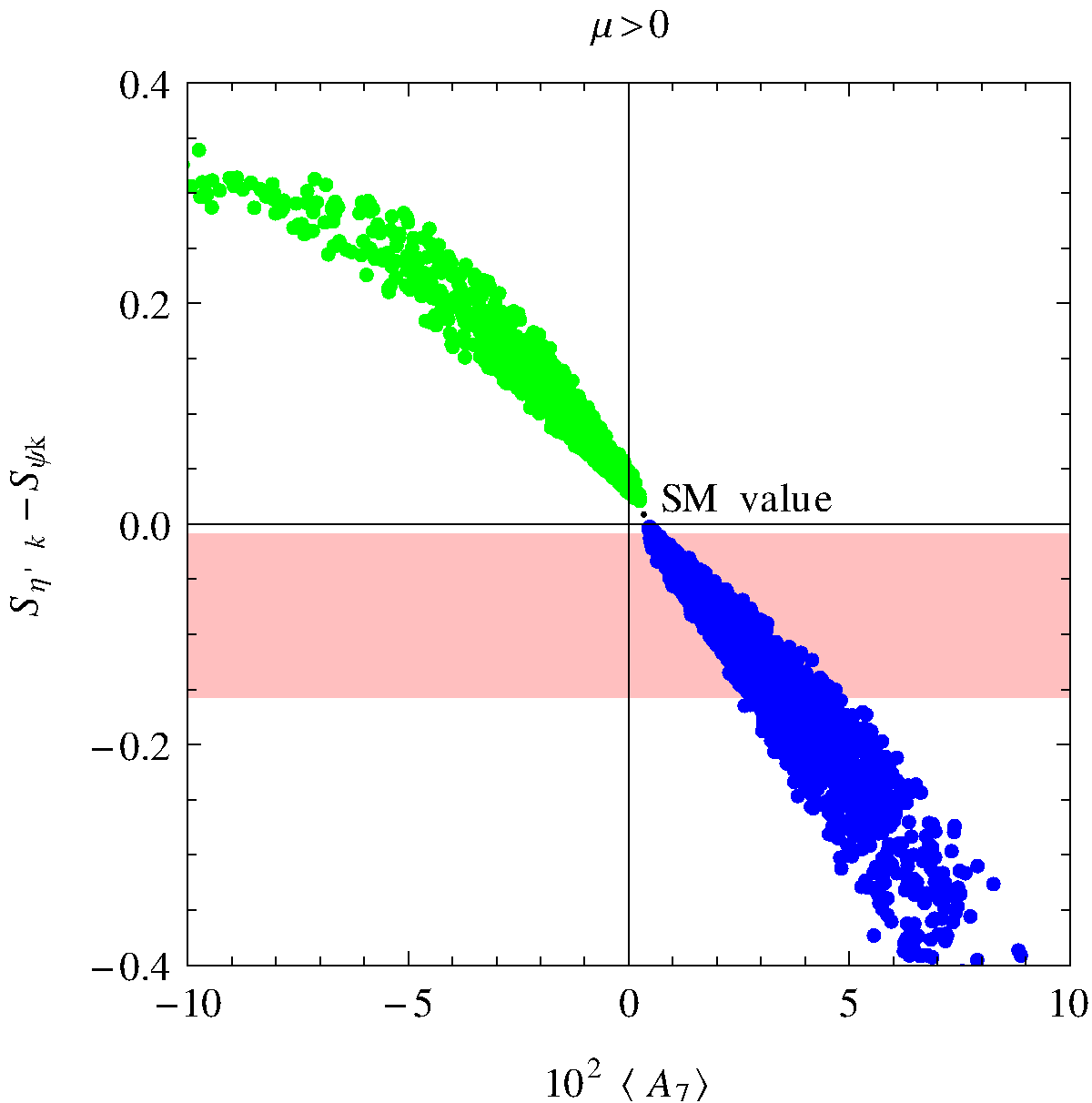
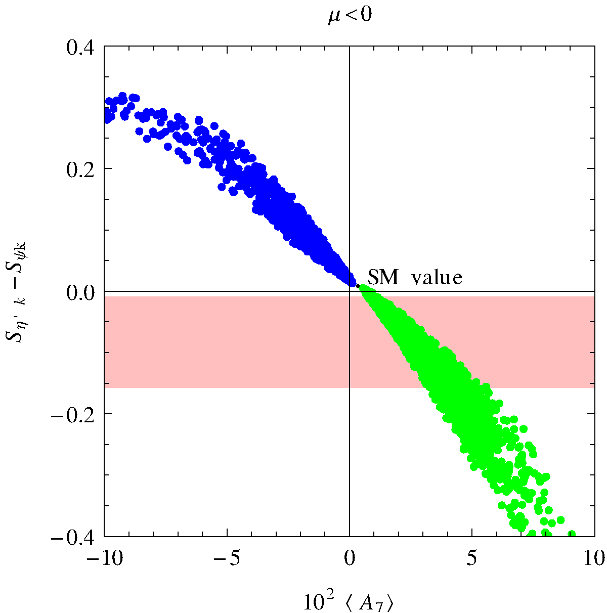
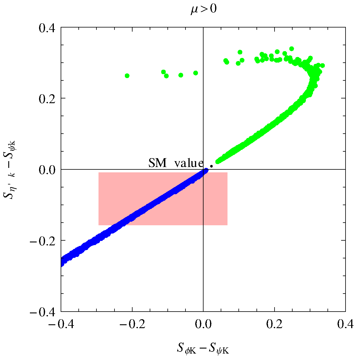
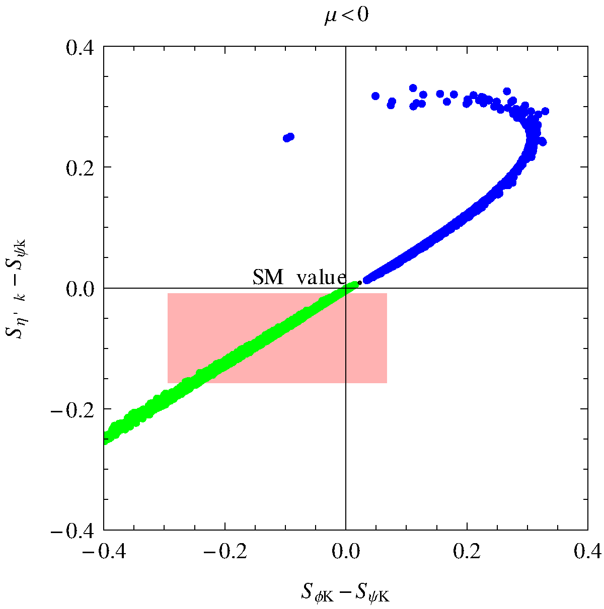
Figure 1: Correlation between SϕKSSψKSsubscript𝑆italic-ϕsubscript𝐾𝑆subscript𝑆𝜓subscript𝐾𝑆S_{\phi K_{S}}-S_{\psi K_{S}} and SηKSSψKSsubscript𝑆superscript𝜂subscript𝐾𝑆subscript𝑆𝜓subscript𝐾𝑆S_{\eta^{\prime}K_{S}}-S_{\psi K_{S}} for positive μ𝜇\mu (left) and negative μ𝜇\mu (right), showing points with γL>0subscript𝛾𝐿0\gamma_{L}>0 (blue) and γL<0subscript𝛾𝐿0\gamma_{L}<0 (green). The shaded region shows the 1σ1𝜎1\sigma experimental ranges.
Refer to caption
Refer to caption
Figure 2: Correlation between A7(BKμ+μ)delimited-⟨⟩subscript𝐴7𝐵superscript𝐾superscript𝜇superscript𝜇\langle A_{7}(B\to K^{*}\mu^{+}\mu^{-})\rangle and the difference SηKSSψKSsubscript𝑆superscript𝜂subscript𝐾𝑆subscript𝑆𝜓subscript𝐾𝑆S_{\eta^{\prime}K_{S}}-S_{\psi K_{S}} for positive μ𝜇\mu (left) and negative μ𝜇\mu (right), showing points with γL>0subscript𝛾𝐿0\gamma_{L}>0 (blue) and γL<0subscript𝛾𝐿0\gamma_{L}<0 (green). The shaded region is the 1σ1𝜎1\sigma experimental range.
Refer to caption
Refer to caption
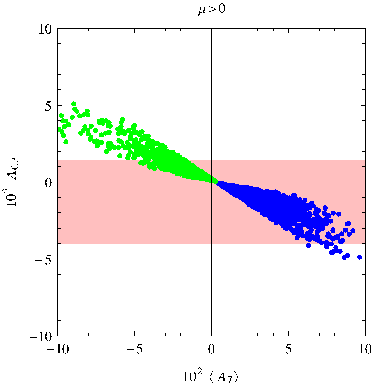
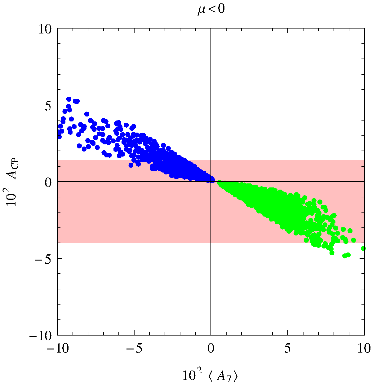
Figure 3: Correlation between A7(BKμ+μ)delimited-⟨⟩subscript𝐴7𝐵superscript𝐾superscript𝜇superscript𝜇\langle A_{7}(B\to K^{*}\mu^{+}\mu^{-})\rangle and the new physics contributions to the CP asymmetry in BXsγ𝐵subscript𝑋𝑠𝛾B\to X_{s}\gamma for positive μ𝜇\mu (left) and negative μ𝜇\mu (right), showing points with γL>0subscript𝛾𝐿0\gamma_{L}>0 (blue) and γL<0subscript𝛾𝐿0\gamma_{L}<0 (green). The shaded region is the 1σ1𝜎1\sigma experimental range for ACP(BXsγ)subscript𝐴CP𝐵subscript𝑋𝑠𝛾A_{\text{CP}}(B\to X_{s}\gamma), valid for vanishing SM contribution (and otherwise subject to an appropriate shift).

4.5 Numerical analysis

In figures 1 and 2 we show the correlations between the CP asymmetries, scanning the gluino mass between 0.5 and 1 TeV, the sbottom mass, the μ𝜇\mu term and Absubscript𝐴𝑏A_{b} between 0.2 and 0.5 TeV and tanβ𝛽\tan\beta between 2 and 10. We require the ΔF=2Δ𝐹2\Delta F=2 observables to be in the region where the CKM tensions are reduced (cf. (1113)). The maximum size of the effects is mostly limited by the BR(BXsγ)BR𝐵subscript𝑋𝑠𝛾\text{BR}(B\to X_{s}\gamma) constraint, which we require to be fulfilled at the 3σ3𝜎3\sigma level including SM and gluino contributions only (cf. the discussion at the end of sec. 4.1).

Figure 1 shows the correlation between the mixing-induced CP asymmetries SϕKSsubscript𝑆italic-ϕsubscript𝐾𝑆S_{\phi K_{S}} and SηKSsubscript𝑆superscript𝜂subscript𝐾𝑆S_{\eta^{\prime}K_{S}} in relation to SψKSsubscript𝑆𝜓subscript𝐾𝑆S_{\psi K_{S}}, effectively subtracting the contribution due to the modified Bdsubscript𝐵𝑑B_{d} mixing phase. The experimental 1σ1𝜎1\sigma ranges corresponding to the average in table 1 are shown as shaded regions. Due to the tanβ𝛽\tan\beta enhanced terms in (4142), large effects are easily possible. A negative value for these differences, as currently indicated by the central values of the measurements, can be obtained for γL>0subscript𝛾𝐿0\gamma_{L}>0 (γL<0subscript𝛾𝐿0\gamma_{L}<0) if μ>0𝜇0\mu>0 (μ<0𝜇0\mu<0). For a given sign of the μ𝜇\mu term, the sign of the ΔB=1Δ𝐵1\Delta B=1 CP asymmetries can thus serve to distinguish between the two solutions for the phase γLsubscript𝛾𝐿\gamma_{L} in (13) allowed by the ΔF=2Δ𝐹2\Delta F=2 analysis.

Figure 2 shows the correlation between SηKSsubscript𝑆superscript𝜂subscript𝐾𝑆S_{\eta^{\prime}K_{S}} and the CP asymmetry A7delimited-⟨⟩subscript𝐴7\langle A_{7}\rangle in BKμ+μ𝐵superscript𝐾superscript𝜇superscript𝜇B\to K^{*}\mu^{+}\mu^{-}. Values up to ±10%plus-or-minuspercent10\pm 10\% would be attainable for A7delimited-⟨⟩subscript𝐴7\langle A_{7}\rangle, while the current measurement of SηKSsubscript𝑆superscript𝜂subscript𝐾𝑆S_{\eta^{\prime}K_{S}} implies, at the 1σ1𝜎1\sigma level, 0<A7<5%0delimited-⟨⟩subscript𝐴7percent50<\langle A_{7}\rangle<5\%.

Finally, figure 3 shows the correlation between the CP asymmetry in BXsγ𝐵subscript𝑋𝑠𝛾B\to X_{s}\gamma and the new physics contribution to A7delimited-⟨⟩subscript𝐴7\langle A_{7}\rangle. ACP(BXsγ)NPsubscript𝐴CPsubscript𝐵subscript𝑋𝑠𝛾NPA_{\text{CP}}(B\to X_{s}\gamma)_{\text{NP}} attains values up to ±5%plus-or-minuspercent5\pm 5\%. Imposing the 1σ1𝜎1\sigma experimental range allowed for SηKSsubscript𝑆superscript𝜂subscript𝐾𝑆S_{\eta^{\prime}K_{S}}, this decreases to 2%<ACP(BXsγ)NP<0%percent2subscript𝐴CPsubscript𝐵subscript𝑋𝑠𝛾NPpercent0-2\%<A_{\text{CP}}(B\to X_{s}\gamma)_{\text{NP}}<0\%. In the plots, we also show the 1σ1𝜎1\sigma experimental range for ACP(BXsγ)subscript𝐴CP𝐵subscript𝑋𝑠𝛾A_{\text{CP}}(B\to X_{s}\gamma) (cf. table 1), assuming a vanishing SM contribution. If the SM contribution is sizable due to long-distance effects (see section 4.2), the experimental constraints has to be shifted accordingly.

5 Discussion and conclusions

We have studied CP asymmetries in B𝐵B decays in supersymmetry with a U(2)3𝑈superscript23U(2)^{3} flavour symmetry suggested in [10] as an alternative to Minimal Flavour Violation, addressing the SUSY flavour and CP problems, partially explaining the hierarchies in the Yukawa couplings and solving tensions in the CKM fit related to CP violation in meson mixing.

Even in the absence of flavour-blind phases, we find potentially sizable CP violating contributions to ΔB=1Δ𝐵1\Delta B=1 decay amplitudes. We identify the dominant contributions to arise in the magnetic and chromomagnetic dipole operators due to their sensitivity to chirality violation, with subleading contributions in semi-leptonic and QCD penguin operators. The most promising observables are the mixing-induced CP asymmetries in non-leptonic penguin decays like BϕKS𝐵italic-ϕsubscript𝐾𝑆B\to\phi K_{S} or BηKS𝐵superscript𝜂subscript𝐾𝑆B\to\eta^{\prime}K_{S}, angular CP asymmetries in BKμ+μ𝐵superscript𝐾superscript𝜇superscript𝜇B\to K^{*}\mu^{+}\mu^{-}, and the direct CP asymmetry in BXsγ𝐵subscript𝑋𝑠𝛾B\to X_{s}\gamma (barring potential uncertainties in controlling the SM predictions in the radiative [15] and non-leptonic modes [17, 18]).

Due to the different dependence on the sparticle masses, we cannot predict a clear-cut correlation between CP violating ΔF=1Δ𝐹1\Delta F=1 and ΔF=2Δ𝐹2\Delta F=2 observables. However, we have demonstrated that observable effects in ΔF=1Δ𝐹1\Delta F=1 CP asymmetries are certainly compatible with the pattern of deviations from the SM suggested by ΔF=2Δ𝐹2\Delta F=2 observables, if interpreted in terms of this supersymmetric framework. Interestingly, while we considered a setup without flavour-blind phases, the correlations between ΔF=1Δ𝐹1\Delta F=1 observables turn out to be very similar to those in MFV [25, 26] or in effective MFV [7] with flavour-blind phases. The main difference between the two cases are the CP violating effects in K𝐾K and B𝐵B mixing, which occur in U(2)3𝑈superscript23U(2)^{3}, but not in (effective) MFV. We view this as an interesting example of the usefulness of correlated studies of ΔF=1Δ𝐹1\Delta F=1 and ΔF=2Δ𝐹2\Delta F=2 observables as a handle to distinguish between models. Such studies would become extremely interesting in presence of direct evidences of a hierarchical sparticle spectrum from the LHC.

Acknowledgments

This work was supported by the EU ITN “Unification in the LHC Era”, contract PITN-GA-2009-237920 (UNILHC) and by MIUR under contract 2008XM9HLM. G.I. acknowledges the support of the Technische Universität München – Institute for Advanced Study, funded by the German Excellence Initiative.

Appendix A Loop functions

fG(x)=2(73134x+37x2)39(x1)32(1827x+x3)13(x1)4lnxsubscript𝑓𝐺𝑥273134𝑥37superscript𝑥239superscript𝑥1321827𝑥superscript𝑥313superscript𝑥14𝑥f_{G}(x)=\dfrac{2(73-134x+37x^{2})}{39(x-1)^{3}}-\dfrac{2(18-27x+x^{3})}{13(x-1)^{4}}\ln x fG(1)=1subscript𝑓𝐺11f_{G}(1)=1
fγ(x)=2(27x+11x2)3(x1)3+4x3(x1)4lnxsubscript𝑓𝛾𝑥227𝑥11superscript𝑥23superscript𝑥134superscript𝑥3superscript𝑥14𝑥f_{\gamma}(x)=-\dfrac{2(2-7x+11x^{2})}{3(x-1)^{3}}+\dfrac{4x^{3}}{(x-1)^{4}}\ln x fγ(1)=1subscript𝑓𝛾11f_{\gamma}(1)=1
f7(x)=2(1+5x+2x2)(x1)312x2(x1)4lnxsubscript𝑓7𝑥215𝑥2superscript𝑥2superscript𝑥1312superscript𝑥2superscript𝑥14𝑥f_{7}(x)=\dfrac{2(-1+5x+2x^{2})}{(x-1)^{3}}-\dfrac{12x^{2}}{(x-1)^{4}}\ln x f7(1)=1subscript𝑓711f_{7}(1)=1
g7(x)=6x(1+5x)(x1)3+12x2(2+x)(x1)4lnxsubscript𝑔7𝑥6𝑥15𝑥superscript𝑥1312superscript𝑥22𝑥superscript𝑥14𝑥g_{7}(x)=-\dfrac{6x(1+5x)}{(x-1)^{3}}+\dfrac{12x^{2}(2+x)}{(x-1)^{4}}\ln x g7(1)=1subscript𝑔711g_{7}(1)=1
f8(x)=1940x+11x25(x1)36x(9+x)5(x1)4lnxsubscript𝑓8𝑥1940𝑥11superscript𝑥25superscript𝑥136𝑥9𝑥5superscript𝑥14𝑥f_{8}(x)=\dfrac{-19-40x+11x^{2}}{5(x-1)^{3}}-\dfrac{6x(-9+x)}{5(x-1)^{4}}\ln x f8(1)=1subscript𝑓811f_{8}(1)=1
g8(x)=12x(11+x)5(x1)3+6x(916x+x2)5(x1)4lnxsubscript𝑔8𝑥12𝑥11𝑥5superscript𝑥136𝑥916𝑥superscript𝑥25superscript𝑥14𝑥g_{8}(x)=\dfrac{12x(11+x)}{5(x-1)^{3}}+\dfrac{6x(-9-16x+x^{2})}{5(x-1)^{4}}\ln x g8(1)=1subscript𝑔811g_{8}(1)=1

References