Sparse Estimation by Exponential Weighting

Abstract

Consider a regression model with fixed design and Gaussian noise where the regression function can potentially be well approximated by a function that admits a sparse representation in a given dictionary. This paper resorts to exponential weights to exploit this underlying sparsity by implementing the principle of sparsity pattern aggregation. This model selection take on sparse estimation allows us to derive sparsity oracle inequalities in several popular frameworks, including ordinary sparsity, fused sparsity and group sparsity. One striking aspect of these theoretical results is that they hold under no condition in the dictionary. Moreover, we describe an efficient implementation of the sparsity pattern aggregation principle that compares favorably to state-of-the-art procedures on some basic numerical examples.

and

1 Introduction

Since the 1990s, the idea of exponential weighting has been successfully used in a variety of statistical problems. In this paper, we review several properties of estimators based on exponential weighting with a particular emphasis on how they can be used to construct optimal and computationally efficient procedures for high-dimensional regression under the sparsity scenario.

Most of the work on exponential weighting deals with a regression learning problem. Some of the results can be extended to other statistical models such as density estimation or classification; cf. Section 6. For the sake of brevity and to make the presentation more transparent, we focus here on the following framework considered in Rigollet and Tsybakov (2011). Let $\mathcal{Z}=\{(x_{1},Y_{1}),\ldots,(x_{n},Y_{n})\}$ be a collection of independent random pairs such that $(x_{i},Y_{i})\in\mathcal{X}\times\mathbb{R}$, where $\mathcal{X}$ is an arbitrary set. Assume the regression model

$$Y_{i}=\eta(x_{i})+\xi_{i},\quad i=1,\ldots,n,$$ (1)

where $\eta\dvtx\mathcal{X}\to\mathbb{R}$ is the unknown regression function, and the errors $\xi_{i}$ are independent Gaussian $\mathcal{N}(0,\sigma^{2})$. The covariates are deterministic elements $x_{1},\ldots,x_{n}$ of $\mathcal{X}$. For any function $f\dvtx\mathcal{X}\to\mathbb{R}$, we define a seminorm $\|\cdot\|$ by

$$\|f\|^{2}=\frac{1}{n}\sum_{i=1}^{n}f^{2}(x_{i}).$$

We adopt the following learning setup. Let $\mathcal{H}=\{f_{1},\ldots,f_{M}\}$, be a dictionary of $M\geq 1$ given functions. For example, $f_{j}$ can be some basis functions or some preliminary estimators of $f$ constructed from another sample that we consider as frozen; see Section 4 for more details. Our goal is to approximate the regression function $\eta$ by a linear combination ${\sf f}_{\theta}(x)=\sum_{j=1}^{M}\theta_{j}f_{j}(x)$ with weights $\theta=(\theta_{1},\dots,\theta_{M})$, where possibly $M\gg n$. The performance of a given estimator $\hat{f}$ of a function $\eta$ is measured in terms of its averaged squared error

$$R(\hat{f})=\|\hat{f}-\eta\|^{2}:=\frac{1}{n}\sum_{i=1}^{n}[\hat{f}(x_{i})-\eta(x_{i})]^{2}.$$

Let $\Theta$ be a given subset of $\mathbb{R}^{M}$. In the aggregation problem, we would ideally wish to find an aggregated estimator $\hat{f}$ whose risk $R(\hat{f})$ is as close as possible in a probabilistic sense to the minimum risk $\inf_{\theta\in\Theta}R(\mathsf{f}_{\theta})$. Namely, one can construct estimators $\hat{f}$ satisfying the following property:

$$\mathbb{E}R(\hat{f})\leq C\inf_{\theta\in\Theta}R(\mathsf{f}_{\theta})+\delta_{n,M}(\Theta),$$ (2)

where $\delta_{n,M}(\Theta)$ is a small remainder term characterizing the performance of the given aggregate $\hat{f}$ and the complexity of the set $\Theta$, $C\geq 1$ is a constant, and $\mathbb{E}$ denotes the expectation. Bounds of the form (2) are called oracle inequalities. In some cases, even more general results are available. They have the form

$$\mathbb{E}R(\hat{f})\leq C\inf_{\theta\in\Theta^{\prime}}\{R(\mathsf{f}_{\theta})+\Delta_{n,M}(\theta)\},$$ (3)

where $\Delta_{n,M}$ is a remainder term that characterizes the performance of the given aggregate $\hat{f}$ and the complexity of the parameter $\theta\in\Theta^{\prime}\subseteq\mathbb{R}^{M}$ (often $\Theta^{\prime}=\mathbb{R}^{M}$). To distinguish from (2), we will call bounds of the form (3) the balanced oracle inequalities. If $\Theta\subseteq\Theta^{\prime}$, then (2) is a direct consequence of (3) with $\delta_{n,M}(\Theta)=C\sup_{\theta\in\Theta}\Delta_{n,M}(\theta)$.

In this paper, we mainly focus on the case where the complexity of a vector $\theta$ is measured as the number of its nonzero coefficients $|\theta|_{0}$. In this case, inequalities of the form (3) are sometimes called sparsity oracle inequalities. Other measures of complexity, also related to sparsity are considered in Section 5.2. As indicated by the notation and illustrated below, the remainder term $\Delta_{n,M}(\theta)$ depends explicitly on the size $M$ of the dictionary and the sample size $n$. It reflects the interplay between these two fundamental parameters and also the complexity of $\theta$.

When the linear model is misspecified, that is, where there is no $\theta\in\Theta$ such that $\eta=\mathsf{f}_{\theta}$ on theset $\{x_{1},\dots,x_{n}\}$, the minimum risk satisfies $\inf_{\theta\in\Theta}R(\mathsf{f}_{\theta})>0$ leading to a systematic bias term. Since this term is unavoidable, we wish to make its contribution as small as possible, and it is therefore important to obtain a leading constant $C=1$. Many oracle inequalities with leading constant $C>1$ can be found in the literature for related problems. However, in most of the papers, the set $\Theta=\Theta_{n}$ depends on the sample size $n$ in such a way that $\inf_{\theta\in\Theta_{n}}R(\mathsf{f}_{\theta})$ tends to $0$ as $n$ goes to infinity, under additional regularity assumptions. In this paper, we are interested in the case where $\Theta$ is fixed. For this reason, we consider here only oracle inequalities with leading constant $C=1$ (called sharp oracle inequalities). Because they hold for finite $M$ and $n$, these are truly finite sample results.

One salient feature of the oracle approach as opposed to standard statistical reasoning, is that it does not rely on an underlying model. Indeed, the goal is not to estimate the parameters of an underlying “true” model but rather to construct an estimator that mimics, in terms of an appropriate oracle inequality, the performance of the best model in a given class, whether this model is true or not. From a statistical viewpoint, this difference is significant since performance cannot be evaluated in terms of parameters. Indeed, there is no true parameter. However, we can still compare the risk of the estimator with the optimum value. Oracle inequalities offer a tool for such a comparison.

A particular choice of $\Theta$ corresponds to the problem of model selection aggregation. Let $\Theta=\Theta^{\rm MC}$ be the set of $M$ canonical basis vectors of $\mathbb{R}^{M}$. Then the set of linear combinations $\{\mathsf{f}_{\theta},\theta\in\Theta^{\rm MC}\}$ coincides with the initial dictionary of functions $\mathcal{H}=\{f_{1},\ldots,f_{M}\}$, so that the goal of model selection is to mimic the best function in the dictionary in the sense of the risk measure $R(\cdot)$. This can be done in different ways, leading to different rates $\delta_{n,M}(\Theta^{\rm MC})$; however one is mostly interested in the methods that attain the rate $\delta_{n,M}^{*}(\Theta^{\rm MC})\asymp(\log M)/n$ which is known to be minimax optimal (see Tsybakov (2003); Bunea, Tsybakov and Wegkamp (2007); Rigollet(2012)). The first sharp oracle inequalities with this rate for a setting different from the one considered here were obtained by Catoni (1999) (see also Catoni (2004)), who used the progressive mixture method based on exponential weighting. Other methods of model selection for aggregation consist in selecting a function in the dictionary by minimizing a (penalized) empirical risk (see, e.g., Nemirovski (2000); Wegkamp (2003); Tsybakov (2003); Lecué (2012)). One of the major novelties offered by exponential weighting is to combine (average) the functions in the dictionary using a convex combination, and not simply to select one of them. From the theoretical point of view, selection of one of the functions has a fundamental drawback since it does not attain the optimal rate $(\log M)/n$; cf. Section 2.

The rest of the paper is organized as follows. In the next section, we discuss some connections between the exponential weighting schemes and penalized empirical risk minimization. In Section 3, we present the first oracle inequalities that demonstrate how exponential weighting can be used to efficiently combine functions in a dictionary. The results of Section 3 are then extended to the case where one wishes to combine not deterministic functions, but estimators. Oracle inequalities for this problem are discussed in Section 4. They are based on the work of Leung and Barron (2006) and Dalalyan and Salmon (2011). Section 5 shows how these results can be adapted to deal with sparsity. We introduce the principle of sparsity pattern aggregation, and we derive sparsity oracle inequalities in several popular frameworks including ordinary sparsity, fused sparsity and group sparsity. Finally, we describe an efficient implementation of the sparsity pattern aggregation principle and compare its performance to state-of-the-art procedures on some basic numerical examples.

2 Exponential Weighting and Penalized Risk Minimization

2.1 Suboptimality of Selectors

A natural candidate to solve the problem of model selection introduced in the previous section is an empirical risk minimizer. Define the empirical risk by

$$\hat{R}_{n}(f)=\frac{1}{n}\sum_{i=1}^{n}[Y_{i}-f(x_{i})]^{2}=\|\mathbf{Y}-f\|^{2}$$

and the empirical risk minimizer by

$$\hat{f}^{\textsc{erm}}=\mathop{\operatorname{argmin}}_{f\in\mathcal{H}}\hat{R}_{n}(f),$$ (4)

where ties are broken arbitrarily. However, while this procedure satisfies an exact oracle inequality, it fails to exhibit the optimal rate of order $\delta_{n,M}^{*}(\Theta^{\rm MC})\asymp(\log M)/n$. The following result shows that this defect is intrinsic not only to empirical risk minimization but also to any method that selects only one function in the dictionary $\mathcal{H}$. This includes methods of model selection by penalized empirical risk minimization. We call estimators $\hat{S}_{n}$, taking values in $\mathcal{H}$ the selectors.

Theorem 2.1

Assume that $\|f_{j}\|\leq 1$ for any $f_{j}\in\mathcal{H}$. Any empirical risk minimizer $\hat{f}^{\textsc{erm}}$ defined in (4) satisfies the following oracle inequality:

$$\qquad\mathbb{E}R(\hat{f}^{\textsc{erm}})\leq\min_{1\leq j\leq M}R(f_{j})+4\sigma\sqrt{\frac{2\log M}{n}}.$$ (5)

Moreover, assume that

$$(\sigma\vee 1)\sqrt{(\log M)/n}\leq C_{0}$$ (6)

for $0<C_{0}<1$ small enough. Then, there exists a dictionary $\mathcal{H}=\{f_{1},\dots,f_{M}\}$ with $\|f_{j}\|\leq 1$, $j=1,\dots,M,$ such that the following holds. For any selector $\hat{S}_{n}$, and in particular, for any selector based on penalized empirical risk minimization, there exists a regression function $\eta$ such that $\|\eta\|\leq 1$ and

$$\mathbb{E}R(\hat{S}_{n})\geq\min_{1\leq j\leq M}R(f_{j})+C_{*}\sigma\sqrt{\frac{\log M}{n}}$$ (7)

for some positive constant $C_{*}$.

See the Appendix.

It follows from the lower bound (7) that selecting one of the functions in a finite dictionary $\mathcal{H}$ to solve the problem of model selection is suboptimal in the sense that it exhibits a too large remainder term, of the order $\sqrt{(\log M)/n}$. It turns out that we can do better if we take a mixture, that is, a convex combination of the functions in $\mathcal{H}$. We will see in Section 3 [cf. (17)] that under a particular choice of weights in this convex combination, namely the exponential weights, one can achieve oracle inequalities with much better rate $(\log M)/n$. This rate is known to be optimal in a minimax sense in several regression setups, including the present one (see Tsybakov (2003); Bunea, Tsybakov and Wegkamp (2007); Rigollet (2012)).

2.2 Exponential Weighting as a Penalized Procedure

Penalized empirical risk minimization for model selection has received a lot of attention in the literature, and many choices for the penalty can be considered (see, e.g., Birgé and Massart (2001); Bartlett, Boucheron and Lugosi (2002); Wegkamp (2003); Lugosi and Wegkamp (2004); Bunea, Tsybakov and Wegkamp (2007)) to obtain oracle inequalities with the optimal or near optimal remainder term. However, all these inequalities exhibit a constant $C>1$ in front of the leading term. This is not surprising as we have proved in the previous section that it is impossible for selectors to satisfy oracle inequalities like (2) that are both sharp (i.e., with $C=1$) and have the optimal remainder term. To overcome this limitation of selectors, we look for estimators obtained as convex combinations of the functions in the dictionary.

The coefficients of convex combinations belong to the flat simplex

$$\Lambda^{M}:=\Biggl{\{}\lambda\in\mathbb{R}^{M}\dvtx\lambda_{j}\geq 0,\sum_{j=1}^{M}\lambda_{j}=1\Biggr{\}}.$$

Let us now examine a few ways to obtain potentially good convex combinations. One candidate is a solution of the following penalized empirical risk minimization problem:

$$\min_{\lambda\in\Lambda^{M}}\{\hat{R}_{n}(\mathsf{f}_{\lambda})+\mathrm{pen}(\lambda)\},$$

where $\mathrm{pen}(\cdot)\geq 0$ is a penalty function. This choice looks quite natural since it provides a proxy of the right-hand side of the oracle inequality (3) where the unknown risk $R(\cdot)$ is replaced by its empirical counterpart $\hat{R}_{n}(\cdot)$. The minimum is taken over the simplex $\Lambda^{M}$ because we are looking for a convex combination. Clearly, the penalty $\mathrm{pen}(\cdot)$ should be carefully chosen and ideally should match the best remainder term $\Delta_{n,M}(\cdot)$. Yet, this problem may be difficult to solve as it involves a minimization over $\Lambda^{M}$. Instead, we propose to solve a simpler problem. Consider the following linear upper bound on the empirical risk:

$$\sum_{j=1}^{M}\lambda_{j}\hat{R}_{n}(f_{j})\geq\hat{R}_{n}(\mathsf{f}_{\lambda})\quad\forall\lambda\in\Lambda^{M}$$

and solve the following optimization problem:

$$\min_{\lambda\in\Lambda^{M}}\Biggl{\{}\sum_{j=1}^{M}\lambda_{j}\hat{R}_{n}(f_{j})+\mathrm{pen}(\lambda)\Biggr{\}}.$$ (8)

Note that if $\mathrm{pen}(\lambda)\equiv 0$, the solution $\hat{\lambda}$ of (8) is simply the empirical risk minimizer over the vertices of the simplex so that $\mathsf{f}_{\hat{\lambda}}=\hat{f}^{\textsc{erm}}$. In general, depending on the penalty function, this problem may be more or less difficult to solve. It turns out that the Kullback–Leibler penalty leads to a particularly simple solution and allows us to approximate the best remainder term $\Delta_{n,M}(\cdot)$ thus adding great flexibility to the resulting estimator.

Observe that vectors in $\Lambda^{M}$ can be associated to probability measures on $\{1,\ldots,M\}$. Let $\lambda=(\lambda_{1},\allowbreak\ldots,\lambda_{M})$ and $\pi=(\pi_{1},\ldots,\pi_{M})$ be two probability measures on $\{1,\ldots,M\}$, and define the Kullback–Leibler divergence between $\lambda$ and $\pi$ by

$$\mathcal{K}(\lambda,\pi)=\sum_{j=1}^{M}\lambda_{j}\log\biggl{(}\frac{\lambda_{j}}{\pi_{j}}\biggr{)}\geq 0.$$

Here and in the sequel, we adopt the convention that $0\log 0=0$, $0\log(a/0)=0$, and $\log(a/0)=\infty$, for any $a>0$.

Exponential weights can be obtained as the solution of the following minimization problem. Fix $\beta>0$, a prior $\pi\in\Lambda^{M}$, and define the vector $\hat{\lambda}^{\pi}$ by

$$\qquad\hat{\lambda}^{\pi}=\mathop{\operatorname{argmin}}_{\lambda\in\Lambda^{M}}\Biggl{\{}\sum_{j=1}^{M}\lambda_{j}\hat{R}_{n}(f_{j})+\frac{\beta}{n}\mathcal{K}(\lambda,\pi)\Biggr{\}}.$$ (9)

This constrained convex optimization problem has a unique solution that can be expressed explicitly. Indeed, it follows from the Karush–Kuhn–Tucker (KKT) conditions that the components $\hat{\lambda}_{j}^{\pi}$ of $\hat{\lambda}^{\pi}$ satisfy

$$n\hat{R}_{n}(f_{j})+\beta\log\biggl{(}\frac{\hat{\lambda}^{\pi}_{j}}{\pi_{j}}\biggr{)}+\mu-\delta_{j}=0,$$ (10)

$$\eqntext{j=1,\ldots,M,}$$ (11)

where $\mu,\delta_{1},\ldots,\delta_{M}\geq 0$ are Lagrange multipliers, and

$$\hat{\lambda}^{\pi}_{j}\geq 0,\quad\delta_{j}\hat{\lambda}^{\pi}_{j}=0,\quad\sum_{j=1}^{M}\hat{\lambda}^{\pi}_{j}=1.$$

Equation (10) together with the above constraints lead to the following closed form solution:

$$\hat{\lambda}^{\pi}_{j}=\frac{\exp(-n\hat{R}_{n}(f_{j})/\beta)\pi_{j}}{\sum_{k=1}^{M}\exp(-n\hat{R}_{n}(f_{k})/\beta)\pi_{k}},$$ (12)

$$\eqntext{j=1,\ldots,M,}$$ (13)

called the exponential weights. We see that one immediate effect of penalizing by the Kullback–Leibler divergence is that the solution of (9) is not a selector. As a result, it achieves the desired effect of averaging as opposed to selecting.

3 Oracle Inequalities

An aggregate is an estimator defined as a weighted average of the functions in the dictionary $\mathcal{H}$ with some data-dependent weights. We focus on the aggregate with exponential weights,

$$\hat{f}^{\pi}=\sum_{j=1}^{M}\hat{\lambda}^{\pi}_{j}f_{j},$$

where $\hat{\lambda}^{\pi}_{j}$ is given in (12). This estimator satisfies the following oracle inequality.

Theorem 3.1

The aggregate $\hat{f}^{\pi}$ with $\beta\geq 4\sigma^{2}$ satisfies the following balanced oracle inequality

$$\hskip 15.0pt\mathbb{E}R(\hat{f}^{\pi})\leq\min_{\lambda\in\Lambda^{M}}\Biggl{\{}\sum_{j=1}^{M}\lambda_{j}R(f_{j})+\frac{\beta}{n}\mathcal{K}(\lambda,\pi)\Biggr{\}}.$$ (14)

Comparing with (9) we see that $\hat{\lambda}^{\pi}$ is the minimizer of the unbiased estimator of the right-hand side of (14). The proof of Theorem 3.1 can be found in the papers of Dalalyan and Tsybakov (2007, 2008) containing more general results. In particular, they apply to non-Gaussian distributions of errors $\xi_{i}$ and to exponential weights with a general (not necessarily discrete) probability distribution $\pi$ on $\mathbb{R}^{M}$. Dalalyan and Tsybakov (2007, 2008) show that the corresponding exponentially weighted aggregate $\hat{f}^{\pi}_{*}$ satisfies the following bound:

$$\hskip 12.0pt\mathbb{E}R(\hat{f}^{\pi}_{*})\leq\inf_{p}\biggl{\{}\int R(\mathsf{f}_{\theta})p({\mathrm{d}}\theta)+\frac{\beta}{n}\mathcal{K}(p,\pi)\biggr{\}},$$ (15)

where the infimum is taken over all probability distributions $p$ on $\mathbb{R}^{M}$, and $\mathcal{K}(p,\pi)$ denotes the Kullback–Leibler divergence between the general probability measures $p$ and $\pi$. Bound (14) follows immediately from (15) by taking $p$ and $\pi$ as discrete distributions.

A useful consequence of (14) can be obtained by restricting the minimum on the right-hand side to the vertices of the simplex $\Lambda^{M}$. These vertices are precisely the vectors $e^{(1)},\ldots,e^{(M)}$ that form the canonical basis of $\mathbb{R}^{M}$ so that

$$\sum_{j=1}^{M}e^{(k)}_{j}R(f_{j})=R(f_{k}),$$

where $e^{(k)}_{j}=\delta_{jk}$ is the $j$th coordinate of $e^{(k)}$, with $\delta_{jk}$ denoting the Kronecker delta. It yields

$$\quad\mathbb{E}R(\hat{f}^{\pi})\leq\min_{1\leq j\leq M}\biggl{\{}R(f_{j})+\frac{\beta}{n}\log(\pi_{j}^{-1})\biggr{\}}.$$ (16)

Taking $\pi$ to be the uniform distribution on $\{1,\ldots,M\}$ leads to the following oracle inequality:

$$\mathbb{E}R(\hat{f}^{\pi})\leq\min_{1\leq j\leq M}R(f_{j})+\frac{\beta\log M}{n},$$ (17)

that exhibits a remainder term of the optimal order $(\log M)/n$.

The role of the distribution $\pi$ is to put a prior weight on the functions in the dictionary. When there is no preference, the uniform prior is a common choice. However, we will see in Section 5 that choosing nonuniform weights depending on suitable sparsity characteristics can be very useful. Moreover, this methodology can be extended to many cases where one wishes to learn with a prior. It is worth mentioning that while the terminology is reminiscent of a Bayesian setup, this paper deals only with a frequentist setting (the risk is not averaged over the prior).

4 Aggregation of Estimators

4.1 From Aggregation of Functions to Aggregation of Estimators

Akin to the setting of the previous section, exponential weights were originally introduced to aggregate deterministic functions $f_{j}$ from a dictionary. These functions can be chosen in essentially two ways. Either they have good approximation properties such as an (over-complete) basis of functions or they are constructed as preliminary estimators using a hold-out sample. The latter case corresponds to the problem of aggregation of estimators originally described in Nemirovski (2000). The idea put forward by Nemirovski (2000) is to obtain two independent samples from the initial one by randomization; estimators are constructed from the first sample while the second is used to perform aggregation. To carry out the analysis of the aggregation step, it is enough to work conditionally on the first sample so that the problem reduces to aggregation of deterministic functions. A limitation is that Nemirovski’s randomization only applies to Gaussian model with known variance. Nevertheless, this idea of two-step procedures carries over to models with i.i.d. observations where one can do direct sample splitting (see, e.g., Yang (2004); Rigollet and Tsybakov (2007); Lecué (2007)). Thus, in many cases aggregation of estimators can be achieved by reduction to aggregation of functions.

Along with this approach, one can aggregate estimators using the same observations for both estimation and aggregation. While for general estimators this would clearly result in overfitting, the idea proved to be successful for certain types of estimators, first for projection estimators (Leung and Barron (2006)) and more recently for a more general class of linear (affine) estimators (Dalalyan and Salmon (2011)). Our further analysis will be based on this approach. Clearly, direct sample splitting does not apply to independent samples that are not identically distributed as in the present setup. Indeed, the observations in the first sample no longer have the same distribution as those in the second sample. On the other hand, the approach based on Nemirovski’s randomization can be still applied, but it leads to somewhat weaker results involving an additional expectation over a randomization distribution and a bigger remainder term than in our oracle inequalities.

4.2 Aggregation of Linear Estimators

Suppose that we are given a finite family $\{\hat{f}_{1},\ldots,\allowbreak\hat{f}_{K}\}$ of linear estimators defined by

$$\hat{f}_{j}(x)=\mathbf{Y}^{\top}a_{j}(x),$$ (18)

where $a_{j}(\cdot)$ are given functions with values in $\mathbb{R}^{n}$. This representation is quite general; for example, $\hat{f}_{j}$ can be ordinary least squares, (kernel) ridge regression estimators or diagonal linear filter estimators; see Kneip (1994); Dalalyan and Salmon (2011) for a longer list of relevant examples. The vector of values $(\hat{f}_{j}(x_{i}),i=1,\dots,n)$ equals to $A_{j}\mathbf{Y}$ where $A_{j}$ an $n\times n$ matrix with rows $a_{j}(x_{i}),i=1,\dots,n$.

Now, we would like to consider mixtures of such estimators rather than mixtures of deterministic functions as in the previous sections. For this purpose, exponential weights have to be slightly modified. Indeed, note that in Section 2, the risk of a deterministic function $f_{j}$ is simply estimated by the empirical risk $\hat{R}_{n}(f_{j})$, which is plugged into the expression for the weights. Clearly, $\mathbb{E}\hat{R}_{n}(f_{j})=R(f_{j})+\sigma^{2}$ so that $\hat{R}_{n}(f_{j})$ is an unbiased estimator of the risk $R(f_{j})$ of $f_{j}$ up to an additive constant. For a linear estimator $\hat{f}_{j}$ defined in (18), $\hat{R}_{n}(\hat{f}_{j})-\sigma^{2}$ is no longer an unbiased estimator of the risk $\mathbb{E}R(\hat{f}_{j})$. It is well known that the risk of the linear estimator $\hat{f}_{j}$ has the form

$$\mathbb{E}R(\hat{f}_{j})=\|(A_{j}-\mathbf{I})\eta\|^{2}+\frac{\sigma^{2}}{n}\operatorname{Tr}[A_{j}^{\top}A_{j}],$$

where $\operatorname{Tr}[A]$ denotes the trace of a matrix $A$, and $\mathbf{I}$ denotes the $n\times n$ identity matrix. Moreover, an unbiased estimator of $\mathbb{E}R(\hat{f}_{j})$ is given by a version of Mallows’s $C_{p}$,

$$\qquad\tilde{R}^{\mathrm{unb}}_{n}(\hat{f}_{j})=\|\mathbf{Y}-\hat{f}_{j}\|^{2}+\frac{2\sigma^{2}}{n}\operatorname{Tr}[A_{j}]-\sigma^{2}.$$ (19)

Then, for linear estimators, the exponential weights and the corresponding aggregate are modified as follows:

$$\hat{\lambda}^{\pi}_{j} = \frac{\exp(-n\tilde{R}^{\mathrm{unb}}_{n}(\hat{f}_{j})/\beta)\pi_{j}}{\sum_{k=1}^{K}\exp(-n\tilde{R}^{\mathrm{unb}}_{n}(\hat{f}_{k})/\beta)\pi_{k}},$$

$$\hat{f}^{\pi} = \sum_{k=1}^{K}\hat{\lambda}^{\pi}_{k}\hat{f}_{k}.$$

Note that for deterministic $f_{j}$, we naturally define $\tilde{R}^{\mathrm{unb}}_{n}(f_{j})=\hat{R}_{n}(f_{j})-\sigma^{2}$, so that definition (4.2) remains consistent with (12). With this more general definition of exponential weights, Dalalyan and Salmon (2011) prove the following risk bounds for the aggregate $\hat{f}^{\pi}$.

Theorem 4.1

Let $\{\hat{f}_{1},\ldots,\hat{f}_{K}\}$ be a family of linear estimators defined in (18) such that the matrices $A_{j}$ are symmetric, positive definite and $A_{j}A_{k}=A_{k}A_{j}$, for all $1\leq j,k\leq K$. Then the exponentially weighted aggregate $\hat{f}^{\pi}$ defined in (4.2) with $\beta\geq 8\sigma^{2}$ satisfies

$$\hskip 19.0pt\mathbb{E}R(\hat{f}^{\pi}) \leq \min_{\lambda\in\Lambda^{K}}\Biggl{\{}\sum_{j=1}^{K}\lambda_{j}\mathbb{E}R(\hat{f}_{j})+\frac{\beta}{n}\mathcal{K}(\lambda,\pi)\Biggr{\}},$$ (21)

$$\mathbb{E}R(\hat{f}^{\pi}) \leq \min_{j=1,\dots,K}\biggl{\{}\mathbb{E}R(\hat{f}_{j})+\frac{\beta}{n}\log(\pi_{j}^{-1})\biggr{\}}.$$ (22)

If all the $A_{j}$ are projection matrices ($A_{j}^{\top}=A_{j}$,$A_{j}^{2}=A_{j}$), then the above inequalities hold with $\beta\geq 4\sigma^{2}$.

Here, bound (22) follows immediately from (21). In the rest of the paper, we mainly use the last part of this theorem concerning projection estimators. The bound (22) for this particular case was originally proved in Leung and Barron (2006). The result of Dalalyan and Salmon (2011) is, in fact, more general than Theorem 4.1 covering nondiscrete priors in the spirit of (15), and it applies not only to linear, but also to affine estimators $\hat{f}_{j}$.

5 Sparse Estimation

The family of projection estimators that we consider in this section is the family of all $2^{M}$ least squares estimators, each of which is characterized by its sparsity pattern. We examine properties of these estimators, and show that their mixtures with exponential weights satisfy sparsity oracle inequalities for suitably chosen priors $\pi$.

5.1 Sparsity Pattern Aggregation

Assume that we are given a dictionary of functions $\mathcal{H}=\{f_{1},\ldots,f_{M}\}$. However, we will not aggregate the elements of the dictionary, but rather the least squares estimators depending on all the $f_{j}$. We denote by $\mathbf{X}$, the $n\times M$ design matrix with elements $\mathbf{X}_{i,j}=f_{j}(x_{i})$, $i=1,\ldots,n,j=1,\ldots,M$.

A sparsity pattern is a binary vector $\mathsf{p}\in\mathcal{P}:=\{0,1\}^{M}$. The terminology comes from the fact that the coordinates $\mathsf{p}_{j}$ of such vectors can be interpreted as indicators of presence ($\mathsf{p}_{j}=1$) or absence ($\mathsf{p}_{j}=0$) of a given feature indexed by $j\in\{1,\ldots,M\}$. We denote by $|\mathsf{p}|$ the number of ones in the sparsity pattern $\mathsf{p}$, and by $S^{\mathsf{p}}$ the linear span of canonical basis vectors $e^{(j)}$, such that $\mathsf{p}_{j}=1$.

For $\mathsf{p}\in\mathcal{P}$, let $\hat{\theta}_{\mathsf{p}}$ be any least squares estimator on $S^{\mathsf{p}}$ defined by

$$\qquad\hat{\theta}_{\mathsf{p}}\in\mathop{\operatorname{argmin}}_{\theta\in S^{\mathsf{p}}}\|\mathbf{Y}-\mathsf{f}_{\theta}\|^{2}\quad\mbox{with }\mathsf{f}_{\theta}=\sum_{j=1}^{M}\theta_{j}f_{j}.$$ (23)

The following simple lemma gives an oracle inequality for the least squares estimator. It follows easily from the Pythagorean theorem. Moreover, the random variables $\xi_{1},\ldots,\xi_{n}$ need not be Gaussian for the result to hold.

Lemma 5.1

Fix $\mathsf{p}\in\mathcal{P}$. Then any least squares estimator $\hat{\theta}_{\mathsf{p}}$ defined in (23) satisfies

$$\mathbb{E}\|\mathsf{f}_{\hat{\theta}_{\mathsf{p}}}-\eta\|^{2} = \min_{\theta\in S^{\mathsf{p}}}\|\mathsf{f}_{\theta}-\eta\|^{2}+\sigma^{2}\frac{d_{\mathsf{p}}}{n}$$

$$\leq \min_{\theta\in S^{\mathsf{p}}}\|\mathsf{f}_{\theta}-\eta\|^{2}+\sigma^{2}\frac{|\mathsf{p}|}{n},$$

where $d_{\mathsf{p}}$ is the dimension of the linear subspace $\{\mathbf{X}\theta\dvtx\theta\in S^{\mathsf{p}}\}$ .

Clearly, if $|\mathsf{p}|$ is small compared to $n$, the oracle inequality gives a good performance guarantee for the least squares aggregate $\mathsf{f}_{\hat{\theta}_{\mathsf{p}}}$. Nevertheless, it may be the case that the approximation error $\min_{\theta\in S^{\mathsf{p}}}\|\mathsf{f}_{\theta}-\eta\|^{2}$ is quite large. Hence, we are looking for a sparsity pattern such that $|\mathsf{p}|$ is small and that yields a least squares aggregate with small approximation error. This is clearly a model selection problem, as described in Section 1.

Observe that for each sparsity pattern $\mathsf{p}\in\mathcal{P}$, the function $\mathsf{f}_{\hat{\theta}_{\mathsf{p}}}$ is a projection estimator of the form $\mathsf{f}_{\hat{\theta}_{\mathsf{p}}}=A_{\mathsf{p}}\mathbf{Y}$ where the $n\times n$ matrix $A_{\mathsf{p}}$ is the projector onto $\{\mathbf{X}\theta\dvtx\theta\in S^{\mathsf{p}}\}$ (as above, we identify the functions $f_{j},\mathsf{f}_{\hat{\theta}_{\mathsf{p}}}$ with the vectors of their values at points $x_{1},\dots,x_{n}$ since the risk depends only on these values). Therefore $\operatorname{Tr}[A_{\mathsf{p}}]=d_{\mathsf{p}}$. We have seen in the previous section that, to solve the problem of model selection, projection estimators can be aggregated using exponential weights. Thus, instead of selecting the best sparsity pattern, we resort to taking convex combinations leading to what is called sparsity pattern aggregation. For any sparsity pattern $\mathsf{p}\in\mathcal{P}$, define the exponential weights $\hat{\lambda}^{\pi}_{\mathsf{p}}$ and the sparsity pattern aggregate $\tilde{f}^{\pi}$, respectively, by

$$\hat{\lambda}^{\pi}_{\mathsf{p}} = \frac{\exp(-n\tilde{R}^{\mathrm{unb}}_{n}(\mathsf{f}_{\hat{\theta}_{\mathsf{p}}})/\beta)\pi_{\mathsf{p}}}{\sum_{\mathsf{p}^{\prime}\in\mathcal{P}}\exp(-n\tilde{R}^{\mathrm{unb}}_{n}(\mathsf{f}_{\hat{\theta}_{\mathsf{p}^{\prime}}})/\beta)\pi_{\mathsf{p}^{\prime}}},$$

$$\tilde{f}^{\pi} = \sum_{\mathsf{p}\in\mathcal{P}}\hat{\lambda}^{\pi}_{\mathsf{p}}\mathsf{f}_{\hat{\theta}_{\mathsf{p}}},$$

where $\pi=(\pi_{\mathsf{p}})_{\mathsf{p}\in\mathcal{P}}$ is a probability distribution (prior) on the set of sparsity patterns $\mathcal{P}$.

To study the performance of this method, we can now apply the last part of Theorem 4.1 dealing with projection matrices. Let $\mathsf{p}(\theta)\in\mathcal{P}$ be the sparsity pattern of $\theta\in\mathbb{R}^{M}$, that is, a vector with components $\mathsf{p}_{j}(\theta)=1$ if $\theta_{j}\neq 0$, and $\mathsf{p}_{j}(\theta)=0$ otherwise. Note that $|\mathsf{p}(\theta)|=|\theta|_{0}$. Combining (22) and Lemma 5.1 and the fact that $\{\theta\dvtx\mathsf{p}(\theta)=\mathsf{p}\}\subset S^{\mathsf{p}}$, we get that for $\beta\geq 4\sigma^{2}$

$$\mathbb{E}R(\tilde{f}^{\pi}) \leq \min_{\mathsf{p}\in\mathcal{P}}\biggl{\{}\mathbb{E}R(\mathsf{f}_{\hat{\theta}_{\mathsf{p}}})+\frac{\beta}{n}\log(\pi_{\mathsf{p}}^{-1})\biggr{\}}$$

$$\leq \min_{\mathsf{p}\in\mathcal{P}}\biggl{\{}\min_{\theta\dvtx\mathsf{p}(\theta)=\mathsf{p}}\|\mathsf{f}_{\theta}-\eta\|^{2}+\sigma^{2}\frac{|\mathsf{p}|}{n}$$

$$\hskip 77.0pt{}+\frac{\beta}{n}\log(\pi_{\mathsf{p}}^{-1})\biggr{\}}$$

$$= \min_{\theta\in\mathbb{R}^{M}}\biggl{\{}\|\mathsf{f}_{\theta}-\eta\|^{2}+\sigma^{2}\frac{|\theta|_{0}}{n}$$

$$\hskip 48.0pt{}+\frac{\beta}{n}\log\bigl{(}\pi_{\mathsf{p}(\theta)}^{-1}\bigr{)}\biggr{\}},$$

where we have used that $\min_{\theta\in\mathbb{R}^{M}}$ can be represented as $\min_{\mathsf{p}\in\mathcal{P}}\min_{\theta\dvtx\mathsf{p}(\theta)=\mathsf{p}}$.

The remainder term in the balanced oracle inequality (5.1) depends on the choice of the prior $\pi$. Several choices can be considered depending on the information that we have about the oracle, that is, about a potentially good candidate $\theta$ that we would like to mimic. For example, we can assume that there exists a good $\theta$ that is coordinatewise sparse, group sparse or even that $\theta$ is piecewise constant. While this approach to structure the prior knowledge seems to fit in a Bayesian framework, we only pursue a frequentist setup. Indeed, our risk measure is not averaged over a prior. Such priors on good candidates for estimation are often used in a non-Bayesian framework. For example, in nonparametric estimation, it is usually assumed that a good candidate function is smooth. Without such assumptions, one may face difficulties in performing meaningful theoretical analysis.

5.2 Sparsity Priors

5.2.1 Coordinatewise sparsity

This is the basicand most commonly used form of sparsity. The prior $\pi$ should favor vectors $\theta$ that have a small numberof nonzero coordinates. Several priors have beensuggested for this purpose; cf. Leung and Barron (2006); Giraud (2007); Rigollet and Tsybakov (2011); Alquier and Lounici (2011). We consider here yet another prior, close to that of Giraud (2007). The main difference is that the prior $\pi^{\textsc{c}}$ below exponentially downweights sparsity patterns with large $|\mathsf{p}|$, whereas the prior in Giraud (2008) downweights such patterns polynomially. Define

$$\pi^{\textsc{c}}_{\mathsf{p}}=\Biggl{[}{M\choose|\mathsf{p}|}e^{|\mathsf{p}|}H_{M}\Biggr{]}^{-1},\quad H_{M}=\sum_{k=0}^{M}e^{-k}\leq\frac{e}{e-1}.$$

It can be easily seen that $\sum_{\mathsf{p}\in\mathcal{P}}\pi^{\textsc{c}}_{\mathsf{p}}=1$ so that $\pi^{\textsc{c}}=(\pi_{\mathsf{p}}^{\textsc{c}},\mathsf{p}\in\mathcal{P})$ is a probability measure on $\mathcal{P}$. Note that

$$\log[(\pi^{\textsc{c}}_{\mathsf{p}})^{-1}] = \log{M\choose|\mathsf{p}|}+|\mathsf{p}|+\log(H_{M})$$

$$\leq 2|\mathsf{p}|\log\biggl{(}\frac{eM}{|\mathsf{p}|}\biggr{)}+\frac{1}{2},$$

where we have used the inequality ${M\choose|\mathsf{p}|}\leq(\frac{eM}{|\mathsf{p}|})^{|\mathsf{p}|}$ for $|\mathsf{p}|\neq 0$ and the convention $0\log(\infty)=0$ for $|\mathsf{p}|=0$. Define the sparsity pattern aggregate

$$\tilde{f}^{\textsc{c}}=\sum_{\mathsf{p}\in\mathcal{P}}\hat{\lambda}^{\pi^{\textsc{c}}}_{\mathsf{p}}\mathsf{f}_{\hat{\theta}_{\mathsf{p}}},$$ (27)

where $\lambda^{\pi^{\textsc{c}}}_{\mathsf{p}}$ is the exponential weight given in (4.2), and $\hat{\theta}_{\mathsf{p}}$ is the least squares estimator (23).

Plugging (5.2.1) into (5.1) with $\pi=\pi^{\textsc{c}}$ and $\beta=4\sigma^{2}$ yields the following sparsity oracle inequality:

$$\qquad\mathbb{E}R(\tilde{f}^{{\textsc{c}}}) \leq \inf_{\theta\in\mathbb{R}^{M}}\biggl{\{}\|\mathsf{f}_{\theta}-\eta\|^{2}$$

$${}+\frac{9\sigma^{2}}{n}|\theta|_{0}\log\biggl{(}\frac{eM}{|\theta|_{0}}\biggr{)}+\frac{2\sigma^{2}}{n}\biggr{\}}.$$

It is important to note that (5.2.1) is valid under no assumption in the dictionary. This is in contrast to the Lasso and assimilated penalized procedures that are known to have similar properties only under strong conditions on $\mathbf{X}$, such as restricted isometry or restricted eigenvalue conditions (see, e.g., Candes and Tao (2007); Bickel, Ritov and Tsybakov (2009); Koltchinskii, Lounici and Tsybakov (2011)).

Another choice for $\pi$ in the framework of coordinatewise sparsity can be found in Rigollet and Tsybakov (2011) and yields the exponential screening estimator. The exponential screening aggregate satisfies an improved version of the above sparsity oracle inequality with $|\theta|_{0}$ replaced by $\min(|\theta|_{0},R)$ where $R$ is the rank of the design matrix $\mathbf{X}$. In particular, if the rank $R$ is small, the exponential screening aggregate adapts to it. Moreover, it is shown in Rigollet and Tsybakov (2011) that the remainder term of the oracle inequality is optimal in a minimax sense.

5.2.2 Fused sparsity

When there exists a natural order among the functions $f_{1},\ldots,f_{M}$ in the dictionary, it may be appropriate to assume that there exists a “piecewise constant” $\theta\in\mathbb{R}^{M}$, that is, $\theta$ with components taking only a small number of values, such that $\mathsf{f}_{\theta}$ has good approximation properties. This property often referred to as fused sparsity has been exploited in the image denoising literature for two decades, originating with the classical paper by Rudin, Osher and Fatemi (1992). The fused Lasso was introduced in Tibshirani et al. (2005) to deal with the same problem in one dimension instead of two. Here we suggest another method that takes advantage of fused sparsity using the idea of mixing with exponential weights. Its theoretical advantages are demonstrated by the sparsity oracle inequality in Corollary 5.1 below.

At first sight, this problem appears to be different from the one considered above since a good $\theta\in\mathbb{R}^{M}$ need not be sparse. Yet, the fused sparsity assumption on $\theta$ can be reformulated into a coordinatewise sparsity assumption. Indeed, let $D$ be the $M\times M$ matrix defined by the relations $(D\theta)_{1}=\theta_{1}$ and $(D\theta)_{j}=\theta_{j}-\theta_{j-1}$ for $j=2,\ldots,M$, where $(D\theta)_{j}$ is the $j$th component of $D\theta$. We will call $D$ the “first differences” matrix. Then $\theta$ is fused sparse if $|D\theta|_{0}$ is small.

We now consider a more general setting with an arbitrary invertible matrix $D$, again declaring $\theta$ to be fused sparse if $|D\theta|_{0}$ is small. Possible definitions of $D$ can be based on higher order differences or combinations of differences of several orders accounting for other types of sparsity. For each sparsity pattern $\mathsf{p}\in\mathcal{P}$, we define the least squares estimator

$$\hat{\theta}_{\mathsf{p}}^{D}\in\mathop{\operatorname{argmin}}_{\theta\in\mathbb{R}^{M}\dvtx D\theta\in S^{\mathsf{p}}}\|\mathbf{Y}-\mathsf{f}_{\theta}\|^{2}.$$ (29)

The corresponding estimator $\mathsf{f}_{\hat{\theta}_{\mathsf{p}}^{D}}$ (as previously, without loss of generality we consider $\mathsf{f}_{\hat{\theta}_{\mathsf{p}}^{D}}$ as an $n$-vector) takes the form $\mathsf{f}_{\hat{\theta}_{\mathsf{p}}^{D}}=A_{\mathsf{p}}^{D}\mathbf{Y}$ where $A_{\mathsf{p}}^{D}$ is the projector onto the linear space $\mathcal{L}_{\mathsf{p}}=\{\mathbf{X}\theta\dvtx\theta\in\mathbb{R}^{M},D\theta\in S^{\mathsf{p}}\}$. In particular, $\operatorname{Tr}[A_{\mathsf{p}}^{D}]=\mathrm{dim}(\mathcal{L}_{\mathsf{p}})$, where $\mathrm{dim}(\mathcal{L}_{\mathsf{p}})$ is the dimension of $\mathcal{L}_{\mathsf{p}}$. Moreover, it is straightforward to obtain the following result, analogous to Lemma 5.1.

Lemma 5.2

Fix $\mathsf{p}\in\mathcal{P}$, and let $D$ be an invertible matrix. Then any least squares estimator $\hat{\theta}_{\mathsf{p}}^{D}$ defined in (29) satisfies

$$\qquad\mathbb{E}\|\mathsf{f}_{\hat{\theta}_{\mathsf{p}}^{D}}-\eta\|^{2} = \mathop{\min_{\theta\in\mathbb{R}^{M}:}}_{D\theta\in S^{\mathsf{p}}}\|\mathsf{f}_{\theta}-\eta\|^{2}+\sigma^{2}\frac{\mathrm{dim}(\mathcal{L}_{\mathsf{p}})}{n}$$

$$\leq \mathop{\min_{\theta\in\mathbb{R}^{M}:}}_{D\theta\in S^{\mathsf{p}}}\|\mathsf{f}_{\theta}-\eta\|^{2}+\sigma^{2}\frac{|\mathsf{p}|}{n}.$$

We are therefore in a position to apply the results from Section 4. For example, if $\mathsf{p}$ is sparse, and $D$ is the “first differences” matrix, the least squares estimator $\hat{\theta}_{\mathsf{p}}^{D}$ is piecewise constant with a small number $|\mathsf{p}|$ of jumps.

Now, since the problem has been reduced to coordinatewise sparsity, we can choose the prior $\pi^{\textsc{c}}$ to favor vectors $\theta\in\mathbb{R}^{M}$ that are piecewise constant with a small number of jumps. Define the fused sparsity pattern aggregate $\tilde{f}^{\textsc{f}}$ by

$$\tilde{f}^{\textsc{f}}=\sum_{\mathsf{p}\in\mathcal{P}}\hat{\lambda}^{\pi^{\textsc{c}}}_{\mathsf{p}}\mathsf{f}_{\hat{\theta}_{\mathsf{p}}^{D}},$$ (31)

where $\hat{\lambda}^{\pi^{\textsc{c}}}_{\mathsf{p}}$ is the exponential weight defined in (4.2), and $\hat{\theta}_{\mathsf{p}}^{D}$ is the least squares estimator defined in (29). Note that we can combine (22) with Lemma 5.2 in the same way as in (5.1) with the only difference that we use now the relation $\min_{\mathsf{p}\in\mathcal{P}}\min_{\theta\dvtx\mathsf{p}(D\theta)=\mathsf{p}}(\cdot)=\min_{\theta\dvtx D\theta\in\mathbb{R}^{M}}(\cdot)=\min_{\theta\in\mathbb{R}^{M}}(\cdot)$. This and (5.2.1) imply the following bound.

Corollary 5.1

Let $D$ be an invertible matrix. The fused sparsity pattern aggregate $\tilde{f}^{\textsc{f}}$ defined in (31) with $\beta=4\sigma^{2}$ satisfies

$$\hskip 20.0pt\mathbb{E}R(\tilde{f}^{{\textsc{f}}})$$

$$\hskip 20.0pt\quad\leq\inf_{\theta\in\mathbb{R}^{M}}\biggl{\{}\|\mathsf{f}_{\theta}-\eta\|^{2}$$ (32)

$$\hskip 20.0pt\quad\hskip 38.0pt{}+\frac{9\sigma^{2}}{n}|D\theta|_{0}\log\biggl{(}\frac{eM}{|D\theta|_{0}}\biggr{)}+\frac{2\sigma^{2}}{n}\biggr{\}}.$$

To our knowledge, analogous bounds for fusedLasso are not available. Furthermore, Corollary 5.1 holds under no assumption on the matrix $\mathbf{X}$, which cannot be the case for the Lasso type methods. Let us also emphasize that Corollary 5.1 is valid for any invertible matrix $D$, and not only for the standard “first differences” matrix $D$ defined above.

5.2.3 Group sparsity

Since recently, estimation under group sparsity has been intensively discussed in the literature. Starting from Yuan and Lin (2006), several estimators have been studied, essentially the Group Lasso and some related penalized techniques. Theoretical properties of the Group Lasso are treated in some generality by Huang and Zhang (2010) and Lounici et al. (2011) where one can find further references. Here we show that one can deal with group sparsity using exponentially weighted aggregates. The new estimator that we propose presents some theoretical advantages as compared to theGroup Lasso type methods.

Let $B_{1},\ldots,B_{K}$ be given subsets of $\{1,\ldots,M\}$ called the groups. We impose no restriction on $B_{j}$’s; for example, they need not form a partition of $\{1,\ldots,M\}$ and can overlap. In this section, we consider $\theta\in\mathbb{R}^{M}$ such that $\operatorname{supp}(\theta)\subseteq B\triangleq\bigcup_{k=1}^{K}B_{k}$ where $\operatorname{supp}(\theta)$ is the support of $\theta$. For any such $\theta$, we denote by $J(\theta)$ the subset of $\{1,\ldots,K\}$ of smallest cardinality among all $J$ satisfying $\operatorname{supp}(\theta)\subseteq B_{J}\triangleq\bigcup_{k\in J}B_{k}$. We assume without loss of generality that $J(\theta)$ is unique. (If there are several $J$ of same cardinality satisfying this property, we define $J(\theta)$ as the smallest among them with respect to some partial ordering of the subsets of $\{1,\ldots,K\}$.) Set

$$g(\theta)=|J(\theta)|,\quad B(\theta)=\bigcup_{k\in J(\theta)}B_{k}.$$

The group sparsity setup assumes that there exists $\theta\in\mathbb{R}^{M}$ such that $\|\mathsf{f}_{\theta}-\eta\|^{2}$ is small and that $\theta$ is supported by a small number of groups, that is, that $g(\theta)\ll K$.

Let now $J$ be a subset $\{1,\ldots,K\}$. Denote by $\mathsf{p}^{J}$ the sparsity pattern with coordinates defined by

$$\mathsf{p}^{J}_{j}=\cases{1,&if $j\in B_{J}$,\cr 0,&otherwise,}$$

for $j=1,\ldots,M$. Consider the set of all such sparsity patterns:

$$\mathcal{P}_{\mathrm{G}}=\bigl{\{}\mathsf{p}^{J},J\subseteq\{1,\ldots,K\}\bigr{\}}.$$

To each sparsity pattern $\mathsf{p}^{J}\in\mathcal{P}_{\mathrm{G}}$ we assign a least squares estimator $\hat{\theta}_{\mathsf{p}^{J}}$, cf. (23), constrained to having null coordinates outside of $B_{J}=\bigcup_{k\in J}B_{k}$.

Define the following prior on $\mathcal{P}_{\mathrm{G}}$:

$$\pi^{\mathrm{G}}_{\mathsf{p}^{J}}=\left[\pmatrix{K\cr|J|}e^{|J|}H_{K}\right]^{-1},\quad J\subseteq\{1,\ldots,K\}.$$

This prior enforces group sparsity by favoring the small number of groups $|J|$. As in (5.2.1), we obtain

$$\log[(\pi^{\mathrm{G}}_{\mathsf{p}^{J}})^{-1}]\leq 2|J|\log\biggl{(}\frac{eK}{|J|}\biggr{)}+\frac{1}{2}.$$ (33)

We introduce now the sparsity pattern aggregate

$$\tilde{f}^{\mathrm{G}}=\sum_{\mathsf{p}\in\mathcal{P}_{\mathrm{G}}}\hat{\lambda}^{\pi^{\mathrm{G}}}_{\mathsf{p}}\mathsf{f}_{\hat{\theta}_{\mathsf{p}}},$$ (34)

where $\lambda^{\pi^{\mathrm{G}}}_{\mathsf{p}}$ is the exponential weight defined in (4.2) and $\hat{\theta}_{\mathsf{p}}$ is the least squares estimator defined in (23).

For any $\mathsf{p}=\mathsf{p}^{J}\in\mathcal{P}_{\mathrm{G}}$, we have $V_{J}\triangleq\{\theta\dvtx\operatorname{supp}(\theta)\subseteq B,J(\theta)=J\}\subseteq S^{\mathsf{p}}$. Arguing as in (5.1) with $\mathcal{P}_{\mathrm{G}}$ instead of $\mathcal{P}$, setting $\pi=\pi^{\mathrm{G}}$ and using (33) we obtain that, for $\beta\geq 4\sigma^{2}$,

$$\mathbb{E}R(\tilde{f}^{{\mathrm{G}}})$$

$$\quad\leq\min_{\mathsf{p}\in\mathcal{P}_{\mathrm{G}}}\biggl{\{}\min_{\theta\in S^{\mathsf{p}}}\|\mathsf{f}_{\theta}-\eta\|^{2}+\sigma^{2}\frac{|\mathsf{p}|}{n}$$

$$\hskip 48.3pt\qquad{}+\frac{\beta}{n}\log((\pi_{\mathsf{p}}^{\mathrm{G}})^{-1})\biggr{\}}$$

$$\quad\leq\min_{J\subseteq\{1,\ldots,K\}}\biggl{\{}\min_{\theta\in V_{J}}\|\mathsf{f}_{\theta}-\eta\|^{2}+\sigma^{2}\frac{|B_{J}|}{n}$$

$$\qquad\hskip 76.4pt{}+\frac{\beta}{n}\log((\pi_{\mathsf{p}^{J}}^{\mathrm{G}})^{-1})\biggr{\}}$$

$$\quad\leq\min_{J\subseteq\{1,\ldots,K\}}\min_{\theta\in V_{J}}\biggl{\{}\|\mathsf{f}_{\theta}-\eta\|^{2}+\sigma^{2}\frac{|B(\theta)|}{n}$$

$$\qquad\hskip 67.5pt{}+\frac{2\beta}{n}g(\theta)\log\biggl{(}\frac{eK}{g(\theta)}\biggr{)}+\frac{\beta}{2n}\biggr{\}}.$$

This leads to the following oracle inequality.

Corollary 5.2

The group sparsity pattern aggregate $\tilde{f}^{\mathrm{G}}$ defined in (34) with $\beta=4\sigma^{2}$ satisfies

$$\mathbb{E}R(\tilde{f}^{{\mathrm{G}}}) \leq \mathop{\inf_{\theta\in\mathbb{R}^{M}:}}_{\operatorname{supp}(\theta)\subseteq B}\biggl{\{}\|\mathsf{f}_{\theta}-\eta\|^{2}+\sigma^{2}\frac{|B(\theta)|+2}{n}$$

$$\qquad\hskip 35.0pt{}+\frac{8\sigma^{2}}{n}g(\theta)\log\biggl{(}\frac{eK}{g(\theta)}\biggr{)}\biggr{\}}.$$

We see from Corollary 5.2 that if there exists an ideal “oracle” $\theta$ in $\mathbb{R}^{M}$, such that the approximation error $\|\mathsf{f}_{\theta}-\eta\|^{2}$ is small, and $\theta$ is sparse in the sense that it is supported by a small number of groups, then the sparsity pattern aggregate $\tilde{f}^{{\textsc{g}}}$ mimics the risk of this oracle.

A remarkable fact is that Corollary 5.2 holds for arbitrary choice of groups $B_{j}$. They can overlap and not necessarily cover the whole set $\{1,\dots,M\}$.

To illustrate the power of the oracle inequality (5.2), we consider the multi-task learning setup as in Lounici et al. (2011). Namely, assume that all the groups $B_{j}$ are of the same size $T$ and form a partition of $\{1,\dots,M\}$, so that $M=KT$. We restrict our analysis to the class $\mathcal{F}_{s}$ of regression functions $\eta$ such that $\eta=\mathsf{f}_{\theta}$ for some $\theta$ satisfying $g(\theta)\leq s$ where $s\leq K$ is a given integer. Then $|B(\theta)|\leq sT$. Combining these remarks with (5.2) and with the fact that the function $x\mapsto x\log(\frac{eK}{x})$ is increasing, we find that, uniformly over $\eta\in\mathcal{F}_{s}$,

$$\qquad\mathbb{E}R(\tilde{f}^{{\textsc{g}}})\leq\frac{\sigma^{2}s}{n}\biggl{(}T+8\log\biggl{(}\frac{eK}{s}\biggr{)}+\frac{2}{s}\biggr{)}.$$ (36)

On the other hand, a minimax lower bound on the same class $\mathcal{F}_{s}$ is available in Lounici et al. (2011). It has exactly the form of the right-hand side of (36); cf. equation (6.2) in Lounici et al. (2011). This immediately implies that (i) the lower bound of Lounici et al. (2011) is tight so that $\frac{s}{n}(T+\log(\frac{K}{s}))$ is the optimal rate of convergence on $\mathcal{F}_{s}$, and (ii) the estimator $\tilde{f}^{{\textsc{g}}}$ is rate optimal. To our knowledge, this gives the first example of rate optimal estimator under group sparsity. The upper bounds for the Group Lasso estimators in Huang and Zhang (2010) and Lounici et al. (2011) as well as in the earlier papers cited therein depart from this optimal rate at least by a logarithmic factor. Furthermore, they are obtained under strong assumptions on the dictionary such as restricted isometry or restricted eigenvalue type conditions, while (36) is valid under no assumption on the dictionary.

6 Related Problems

In this paper, we have considered only the Gaussian regression model with fixed design and known variance of the noise. This is a basic setup where the sharpest results, expressed in terms of sparsity oracle inequalities, are now available for exponentially weighted (EW) procedures both in aggregation and sparsity scenarios. Similar but somewhat weaker properties are obtained for exponential weighting in several other models.

Models with i.i.d. observations. Some EW aggregates achieve sparsity oracle inequalities in regression model with random design (Dalalyan and Tsybakov (2012); Alquier and Lounici (2011); Gerchinovitz (2011)) as well as in density estimation and classification problems (Dalalyan and Tsybakov(2012)). However, the results differ in several aspects from those of the present paper. First, they do not use aggregation of estimators, but rather EW procedures driven by continuous priors (Dalalyan and Tsybakov (2012); Gerchinovitz (2011)), or by priors with both discrete and continuous components (Alquier and Lounici (2011)). The developments in Dalalyan and Tsybakov (2012); Alquier and Lounici (2011); Gerchinovitz (2011) start from the general oracle inequalities similar to (15), which are sometimes called PAC-bounds; cf. recent overview inCatoni (2007). Sparsity oracle inequalities are then derived from PAC-bounds. However, as opposedto (5.2.1), they involve not only $|\theta|_{0}$ but also the $\ell_{1}$-norm of $\theta$. The estimators in Dalalyan and Tsybakov (2012); Gerchinovitz (2011) are defined as an average of exponentially weighted aggregates over the sample sizes from 1 to $n$. This is related to earlier work on mirror averaging; cf. Juditsky et al. (2005); Juditsky, Rigollet and Tsybakov (2008), which in turn, is inspired by the concept of mirror descent in optimization due to Nemirovski. Finally, the computational algorithms are also quite different from those that we describe in the next section. For example, under continuous sparsity priors, one of the suggestions is to use Langevin Monte-Carlo; cf. Dalalyan and Tsybakov (2012, 2012).

Unknown variance of the noise, non-Gaussiannoise. Modifications of EW procedures and of the corresponding oracle inequalities for the case of unknown variance $\sigma^{2}$ are discussed in Giraud (2007); Gerchinovitz (2011). Moreover, the results can be extended to regression with non-Gaussian noise under deterministic or random design (Dalalyan and Tsybakov (2007); Dalalyan and Tsybakov (2008); Dalalyan and Tsybakov (2012); Gerchinovitz (2011)). In particular, Gerchinovitz (2011) uses a version of the EW estimator with data-driven truncation to cover a rather general noise structure. The estimator satisfies a balanced oracle inequality but not a sparsity oracle inequality as defined here, since along with $|\theta|_{0}$, it involves other characteristics of $\theta$ and of the target function $\eta$.

7 Numerical Implementation

All the sparsity pattern aggregates defined in the previous section are of the form $\mathsf{f}_{\theta^{\exp}}$, where

$$\theta^{\exp}=\sum_{\mathsf{p}\in\mathcal{G}}\hat{\lambda}_{\mathsf{p}}^{\pi}\bar{\theta}_{\mathsf{p}}$$ (37)

for some $\mathcal{G}\subset\mathcal{P}$, $\lambda_{\mathsf{p}}^{\pi}$ is the exponential weight defined in (4.2), and $\bar{\theta}_{\mathsf{p}}$ is either $\hat{\theta}_{\mathsf{p}}$ defined in (23) or $\hat{\theta}_{\mathsf{p}}^{D}$ defined in (29).

From (37), it is clear that one needs to add up with some weights $2^{M}$ (or $2^{K}$ in the case of group sparsity with $K$ groups) least squares estimators to compute $\theta^{\exp}$ exactly. In many applications this number is prohibitively large. However, most of the terms in the sum receive an exponentially low weight with the choices of $\pi$ that we have described. We resort to a numerical approximation that exploits this fact.

Note that $\theta^{\exp}$ is obtained as the expectation of the random variable $\hat{\theta}_{\sf P}$ or $\hat{\theta}_{\mathsf{p}}^{D}$ where ${\sf P}$ is a random variable taking values in $\mathcal{P}$ with probability distribution $\nu$ given by

$$\nu_{\mathsf{p}}=\frac{\exp(-n\tilde{R}^{\mathrm{unb}}_{n}(\mathsf{f}_{\bar{\theta}_{\mathsf{p}}})/\beta)\pi_{\mathsf{p}}}{\sum_{\mathsf{p}^{\prime}\in\mathcal{G}}\exp(-n\tilde{R}^{\mathrm{unb}}_{n}(\mathsf{f}_{\bar{\theta}_{\mathsf{p}^{\prime}}})/\beta)\pi_{\mathsf{p}^{\prime}}},\quad\mathsf{p}\in\mathcal{G}\subset\mathcal{P}.$$

This Gibbs-type distribution can be expressed as the stationary distribution of the Markov chain generated by the Metropolis–Hastings (MH) algorithm (see, e.g., Robert and Casella (2004), Section 7.3). We now describe the MH algorithm employed here. Note that in the examples considered in the previous section, $\mathcal{G}$ is either the hypercube $\mathcal{P}$ or the hypercube $\mathcal{P}_{\textsc{g}}$. For any $\mathsf{p}\in\mathcal{G}$, define the instrumental distribution $q(\cdot|\mathsf{p})$ as the uniform distribution on the neighbors of $\mathsf{p}$ in $\mathcal{G}$, and notice that since each vertex has the same number of neighbors, we have $q(\mathsf{p}|\mathsf{q})=q(\mathsf{q}|\mathsf{p})$ for any $\mathsf{p},\mathsf{q}\in\mathcal{P}$. The MH algorithm is defined in Figure 1. We use here the uniform instrumental distribution for the sake of simplicity. Our simulations show that it yields satisfactory results both in terms of performance and of speed. Another choice of $q(\cdot|\cdot)$ can potentially further accelerate the convergence of the MH algorithm.

Fix $\mathsf{p}_{0}=0\in\mathbb{R}^{M}$. For any $t\geq 0$, given $\mathsf{p}_{t}\in\mathcal{G}$: [(3)] (1) Generate a random variable $\mathsf{Q}_{t}$ with distribution $q(\cdot|\mathsf{p}_{t})$. (2) Generate a random variable $$\mathsf{P}_{t+1}=\cases{\mathsf{Q}_{t},&with probability $r(\mathsf{p}_{t},\mathsf{Q}_{t})$,\cr\mathsf{p}_{t},&with probability $1-r(\mathsf{p}_{t},\mathsf{Q}_{t})$,}$$ where $$r(\mathsf{p},\mathsf{q})=\min\biggl{(}\frac{\nu_{\mathsf{q}}}{\nu_{\mathsf{p}}},1\biggr{)}.$$ (3) Compute the least squares estimator $\bar{\theta}_{\mathsf{P}_{t+1}}$.

Figure 1: The Metropolis–Hastings algorithm on the $M$-hypercube.

From the results of Robert and Casella (2004) (see also Rigollet and Tsybakov (2011), Theorem 7.1) the Markov chain $(\mathsf{P}_{t})_{t\geq 0}$ defined in Figure 1 is ergodic. In other words, it holds

$$\lim_{T\to\infty}\frac{1}{T}\sum_{t=T_{0}+1}^{T_{0}+T}\bar{\theta}_{\mathsf{P}_{t}}=\sum_{\mathsf{p}\in\mathcal{G}}\bar{\theta}_{\mathsf{p}}\nu_{\mathsf{p}},\quad\mbox{almost surely},$$

where $T_{0}\geq 0$ is an arbitrary integer.

In view of this result, we approximate $\theta^{\exp}=\break\sum_{\mathsf{p}\in\mathcal{G}}\bar{\theta}_{\mathsf{p}}\nu_{\mathsf{p}}$ by

$$\tilde{\theta}^{\exp}_{T}=\frac{1}{T}\sum_{t=T_{0}+1}^{T_{0}+T}\bar{\theta}_{\mathsf{P}_{t}},$$

which is close to ${\theta^{\exp}}$ for sufficiently large $T$. One remarkable feature of the MH algorithm is that it involves only the ratios $\nu_{\mathsf{q}}/\nu_{\mathsf{p}}$ where $\mathsf{p}$ and $\mathsf{q}$ are two neighbors in $\mathcal{G}$. Such ratios are easy to compute, at least in the examples given in the previous section. As a result, the MH algorithm in this case takes the form of a stochastic greedy algorithm with averaging, which measures a trade-off between sparsity and prediction to decide whether to add or remove a variable. In all subsequent examples, we use a pure R implementation of the sparsity pattern aggregates. While the benchmark estimators considered below employ a C based code optimized for speed, we observed that a safe implementation of the MH algorithm (three times more iterations than needed) exhibits an increase of computation time of at most a factor two.

7.1 Numerical Experiments

The aim of this subsection is to illustrate the performance of the sparsity pattern aggregates $\tilde{f}^{\textsc{c}}$ and $\tilde{f}^{\textsc{f}}$ defined in (27) and (31) respectively, on a simulated dataset and to compare it with state-of-the-art procedures in sparse estimation. In our implementation, we replace the prior $\pi^{\textsc{c}}$ by the exponential screening prior employed in Rigollet and Tsybakov (2011). As a result, the following results are about the exponential screening (es) aggregate defined in Rigollet and Tsybakov (2011). Nevertheless, it presents the same qualitative behavior as the aggregates constructed above.

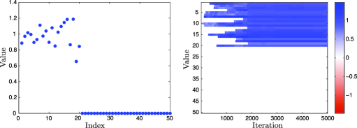
Figure 2: Typical realization for $(M,n,S)=(500,200,20)$. Left: Value of the $\tilde{\theta}^{\exp}_{T}$, $T_{0}=3000,T=7000$. Right: Value of $\hat{\theta}_{\mathsf{P}_{t}}$ for $t=1,\ldots,5000$. Only the first 50 coordinates are shown for each vector.

While our results for the es estimator hold under no assumption on the dictionary, we compare the behavior of our algorithm in a well-known example where sparse estimation by $\ell_{1}$-penalized techniques is theoretically achievable.

Consider the model $\mathbf{Y}=\mathbf{X}\theta^{*}+\sigma\xi$, where $\mathbf{X}$ is an $n\times M$ matrix with independent standard Gaussian entries, and $\xi\in\mathbb{R}^{n}$ is a vector of independent standard Gaussian random variables and is independent of $\mathbf{X}$. Depending on our sparsity assumption, we choose two different $\theta^{*}$.

The variance is chosen as $\sigma^{2}=\|\mathsf{f}_{\theta^{*}}\|^{2}/9=|\mathbf{X}{\theta^{*}}|_{2}^{2}/\allowbreak(9n)$ following the numerical experiments of Candes and Tao [(2007), Section 4]. Here $|\cdot|_{2}$ denotes the $\ell_{2}$ norm. For different values of $(n,M,S)$, we run the es algorithm on 500 replications of the problem and compare our results with several other popular estimators in the literature on sparse estimation that are readily implemented in R. The considered estimators are:

the Lasso estimator with regularization parameter obtained by ten-fold cross-validation;

the mc$+$ estimator of Zhang (2010) with regularization parameter obtained by ten-fold cross-validation;

the scad estimator of Fan and Li (2001) with regularization parameter obtained by ten-fold cross-validation. The Lasso estimator is calculated using the glmnet package in R (Friedman, Hastie and Tibshirani(2010)). The cross-validated mc$+$ and scad estimators are implemented in the ncvreg package in R (Breheny and Huang (2011)).

The performance of each of the four estimators, generically denoted by $\hat{\theta}$ is measured by its prediction error $|\mathbf{X}(\hat{\theta}-\theta^{*})|_{2}^{2}/n=\|{\sf f}_{\hat{\theta}}-{\sf f}_{\theta^{*}}\|^{2}$. Moreover, even though the estimation error $|\hat{\theta}-\theta^{*}|_{2}^{2}$ is not studied above, we also report its values for a better comparison with other simulation studies.

7.1.1 Coordinatewise sparsity

The vector $\theta^{*}$ isgiven by $\theta^{*}_{j}=\mathbh{1}(j\leq S)$ for some fixed $S$ so that $|\theta^{*}|_{0}=S$. Here, $\mathbh{1}(\cdot)$ denotes the indicator function.

Figure 3: Boxplots of performance measure over 500 realizations for the es, Lasso, mc$+$ and scad estimators. Top: estimation performance $|\hat{\theta}-\theta^{*}|_{2}^{2}$. Bottom: Prediction performance: $|\mathbf{X}(\hat{\theta}-\theta^{*})|_{2}^{2}/n$. Left: $(M,n,S)=(200,100,10)$. Right: $(M,n,S)=(500,200,20)$.

We considered the cases $(n,M,S)\in\{(100,200,10),\allowbreak(200,500,20)\}$. The Metropolis approximation $\tilde{\theta}^{\exp}_{T}$ was computed with $T_{0}=3000,T=7000$, which should be in the asymptotic regime of the Markov chain since Figure 2 shows that, on a typical example, the right sparsity pattern is recovered after about 2000 iterations.

Figure 3 displays comparative boxplots, and Table 1 reports averages and standard deviations over the 500 repetitions. In particular, it shows that es outperforms the Lasso estimator and has performance similar to mc$+$ and scad.

Figure 2 illustrates a typical behavior of the es estimator for one particular realization of $\mathbf{X}$ and $\xi$. For better visibility, both displays represent only the 50 first coordinates of $\tilde{\theta}^{\exp}_{T}$, with $T_{0}=3000,T=7000$. The left-hand side display shows that the sparsity pattern is well recovered and the estimated values are close to one. The right-hand side display illustrates the evolution of the intermediate parameter $\hat{\theta}_{\mathsf{P}_{t}}$ for $t=1,\ldots,5000$. It is clear that the Markov chain that runs on the $M$-hypercube graph gets“trapped” in the vertex that corresponds to the sparsity pattern of $\theta^{*}$ after only $2000$ iterations. As a result, while the es estimator is not sparse itself, the MH approximation to the es estimator may output a sparse solution.

Table 1: Means and standard deviations of performance measures over 500 realizations for the es, Lasso, mc$+$ and scad estimators. Top: estimation performance $|\hat{\theta}-\theta^{*}|_{2}^{2}$. Bottom: Prediction performance: $|\mathbf{X}(\hat{\theta}-\theta^{*})|_{2}^{2}/n$

$\bolds{(M,n,S)}$	es	Lasso	mc$+$	scad
$(200,100,10)$	0.14	0.82	0.18	0.17
	(0.11)	(0.28)	(0.17)	(0.15)
$(500,200,20)$	0.29	1.78	0.31	0.29
	(0.16)	(0.43)	(0.14)	(0.12)
$(200,100,10)$	0.12	0.50	0.15	0.14
	(0.08)	(0.15)	(0.10)	(0.10)
$(500,200,20)$	0.25	1.02	0.27	0.26
	(0.11)	(0.22)	(0.11)	(0.10)

The vector $\theta^{*}$ is chosen piecewise constant as follows. Fix an integer $S\geq 1$ such that $10S\leq M$ and consider the blocks $I_{1},\ldots,I_{S}$ defined by

$$I_{j}=\{10(j-1)+1,\ldots,10j\},\quad j=1,\dots,S.$$

The vector $\theta^{*}$ is defined to take value $(-1)^{j}$ on $I_{j},j=1,\ldots,S$ and $1/2$ elsewhere. We considered the cases $(M,n,S)\in\{(200,100,10),(500,200,20)\}$ that are illustrated in Figure 4. Note that in both cases, the vector $\theta^{*}$ is not sparse.

The fused versions of Lasso, mc$+$ and scad are not readily available in R, and we implement them as follows. Recall that $D$ is the $M\times M$ matrix defined in Section 5.2 by $(D\theta)_{1}=\theta_{1}$ and $(D\theta)_{j}=\theta_{j}-\theta_{j-1}$ for $j=2,\ldots,M$. The inverse $D^{-1}$ is the $M\times M$ lower triangular matrix with ones on the diagonal and in the lower triangle. To obtain the fused versions of Lasso, mc$+$ and scad, we simply run these algorithms on the design matrix $\mathbf{X}D^{-1}$ to obtain a solution $\hat{\theta}$. We then return the vector $D^{-1}\hat{\theta}$ as a solution to the fused problem.

We report the boxplots of the two performance measures $|\mathbf{X}(\hat{\theta}-\theta^{*})|_{2}^{2}/n$ and $|\hat{\theta}-\theta^{*}|_{2}^{2}$ in Figure 5. It is clear that, in this example, Exponential Screening outperforms the three other estimators. Moreover, mc$+$ and scad perform particularly poorly in the case $(M,n,S)=(500,200,20)$. Their output on a typical example is illustrated in Figure 4. We can see that they yield an estimator that takes only two values, thus missing most of the structure of the problem. It seems that this behavior can be explained by the fact that the estimators are trapped in a local minimum close to zero.

Appendix

The proof of (5) is standard, and similar results have been formulated in the literature for various other setups. We give it here for the sake of completeness. From the definition of the empirical risk minimizer $\hat{f}^{\textsc{erm}}$, we have

$$\hat{R}_{n}(\hat{f}^{\textsc{erm}})\leq\hat{R}_{n}(f^{*}),$$

where $f^{*}$ is any minimizer of the true risk $R(\cdot)$ over $\mathcal{H}$. Simple algebra yields

$$R(\hat{f}^{\textsc{erm}})\leq R(f^{*})+2\mathbb{E}\langle\hat{f}^{\textsc{erm}}-f^{*},\mathbf{Y}-\eta\rangle,$$

where for two functions $f,g$ from $\mathcal{X}$ to $\mathbb{R}$ we set $\langle f,g\rangle=\frac{1}{n}\sum_{i=1}^{n}f(x_{i})g(x_{i})$. Next, observe that

$$\mathbb{E}\langle\hat{f}^{\textsc{erm}}-f^{*},\mathbf{Y}-\eta\rangle \leq \mathbb{E}\max_{f\in\mathcal{H}}\langle f-f^{*},\mathbf{Y}-\eta\rangle$$

$$\leq 2\sigma\sqrt{\frac{2\log M}{n}},$$

where we used the fact that $\|f^{*}-f\|\leq 2$ for any $f\in\mathcal{H}$, and the inequality $\mathbb{E}[\max_{1\leq i\leq M}a_{i}^{\top}\xi]\leq\sigma\cdot\allowbreak\sqrt{2\log M}$ valid for any $a_{1},\ldots,a_{n}\in\mathbb{R}^{n}$, $|a_{i}|_{2}\leq 1$, where $\xi=(\xi_{1},\ldots,\xi_{n})^{\top}$.

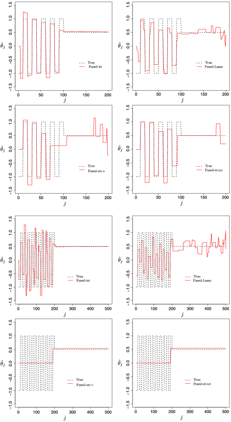
Figure 4: Typical realizations of the fused estimators in the cases $(M,n,S)=(200,100,10)$ (top) and $(M,n,S)=(500,200,20)$ (bottom).

Figure 5: Boxplots of performance measure over 500 realizations for the Fused-es, Fused-Lasso, Fused-mc$+$ and Fused-scad estimators. Top: estimation performance $|\hat{\theta}-\theta^{*}|_{2}^{2}$. Bottom: Prediction performance: $|\mathbf{X}(\hat{\theta}-\theta^{*})|_{2}^{2}/n$. Left: $(M,n,S)=(200,100,10)$. Right: $(M,n,S)=(500,200,20)$.

We now turn to the proof of (7). Consider the random matrix $\mathbb{X}$ of size $n\times M$ such that its elements $\mathbb{X}_{i,j},i=1,\ldots,n,j=1,\ldots,M$ are i.i.d. Rademacher random variables, that is, random variables taking values $1$ and $-1$ with probability $1/2$. Moreover, assume that

$$\frac{2}{n}\log\biggl{(}1+\frac{eM}{2}\biggr{)}<C_{1},$$ (8.1)

for some positive constant $C_{1}<1/2$. Note that (8.1) follows from (6) if $C_{0}$ is chosen small enough. Theorem 5.2 in Baraniuk et al. (2008) (see also Section 5.2.1 in Rigollet and Tsybakov (2011)) entails that if (8.1) holds for $C_{1}$ small enough, then there exists a nonempty set $\mathcal{M}$ of matrices obtained as realizations of the matrix $\mathbb{X}$ that enjoy the following weak restricted isometry (wri) property. For any $X\in\mathcal{M}$, there exists constants $\underline{\kappa}\geq\bar{\kappa}>0$, such that for any $\lambda\in\mathbb{R}^{M}$ with at most $2$ nonzero coordinates,

$$\underline{\kappa}^{2}|\lambda|_{2}^{2}\leq\frac{|X\lambda|_{2}^{2}}{n}\leq\bar{\kappa}^{2}|\lambda|_{2}^{2},$$ (8.2)

when (8.1) is satisfied. For $X\in\mathcal{M}$, let $\phi_{1},\ldots,\phi_{M}$ be any functions on $\mathcal{X}$ satisfying

$$\phi_{j}(x_{i})=X_{i,j},\quad i=1,\ldots,n,j=1,\ldots,M,$$

where $X_{i,j}$ are the entries of $X$. Note that $\|\phi_{j}\|=1$ since $X_{i,j}\in\{-1,1\}$.

Fix $\tau>0$ to be chosen later, and set

$$f_{j}=\tau(1+\alpha)\phi_{j},\quad j=1,\dots,M,$$

where we set for brevity $\alpha=(\sigma/3)\sqrt{\frac{\log M}{\bar{\kappa}^{2}n}}$. Moreover, consider the functions

$$\eta_{j}=\tau\alpha\phi_{j},\quad j=1,\dots,M.$$

Using (6) we choose $\tau$ small enough to ensure that $\|\eta_{j}\|\leq 1$ and $\|f_{j}\|\leq 1$ for any $j=1,\ldots,M$.

We write $R_{j}(\cdot)$ to denote the risk function $R(\cdot)$ when $\eta=\eta_{j}$ in (1). It is easy to check that

$$\min_{f\in\mathcal{H}}R_{j}(f)=R_{j}(f_{j})=\|f_{j}-\eta_{j}\|^{2}.$$ (8.3)

As it is customary in the proof of minimax lower bounds, we reduce our estimation problem to a testing problem as follows. Let $\psi\in\{1,\ldots,M\}$ be the random variable, or test, defined by $\psi=j$ if and only if $\hat{S}_{n}=f_{j}$. Then, $\psi\neq j$ implies that there exists $k\neq j$ such that $\hat{S}_{n}=f_{k}$, so that

$$\|\hat{S}_{n}-\eta_{j}\|^{2}-\|f_{j}-\eta_{j}\|^{2}$$

$$\quad=\|f_{k}-f_{j}\|^{2}+2\langle f_{k}-f_{j},f_{j}-\eta_{j}\rangle$$

$$\quad=\tau^{2}(1+\alpha)^{2}\|\phi_{j}-\phi_{k}\|^{2}$$

$$\qquad{}+2\tau^{2}(1+\alpha)(\langle\phi_{j},\phi_{k}\rangle-1)$$

$$\quad\geq\tau^{2}\alpha\|\phi_{j}-\phi_{k}\|^{2}.$$

From (8.2), we find that $\|\phi_{j}-\phi_{k}\|^{2}\geq 2\underline{\kappa}^{2}$ so that

$$\|\hat{S}_{n}-\eta_{j}\|^{2}-\|f_{j}-\eta_{j}\|^{2}\geq\frac{2\tau^{2}\underline{\kappa}^{2}\sigma}{3\bar{\kappa}}\sqrt{\frac{\log M}{n}}\triangleq\nu_{n,M}.$$

Therefore, we conclude that $\psi\neq j$ implies that

$$R_{j}(\hat{S}_{n})-\min_{f\in\mathcal{H}}R_{j}(f)\geq\nu_{n,M}.$$

Hence,

$$\max_{1\leq j\leq M}P_{j}\Bigl{\{}R_{j}(\hat{S}_{n})-\min_{f\in\mathcal{H}}R_{j}(f)\geq\nu_{n,M}\Bigr{\}}$$

(8.4)

$$\quad\geq\inf_{\psi}\max_{1\leq j\leq M}P_{j}(\psi\neq j),$$

where the infimum is taken over all tests taking values in $\{1,\ldots,M\}$, and $P_{j}$ denotes the joint distribution of $Y_{1},\ldots,Y_{n}$ that are independent Gaussian random variables with mean $\eta_{j}(x_{i})$, respectively. It follows from Tsybakov [(2009), Proposition 2.3 and Theorem 2.5] that if for any $1\leq j,k\leq M$, the Kullback–Leibler divergence between $P_{j}$ and $P_{k}$ satisfies

$$\mathcal{K}(P_{j},P_{k})<\frac{\log M}{8},$$ (8.5)

then there exists a constant $C>0$ such that

$$\inf_{\psi}\max_{1\leq j\leq M}P_{j}(\psi\neq j)\geq C.$$ (8.6)

To check (8.5), observe that, choosing $\tau\leq 1$ and applying (8.2), we get

$$\mathcal{K}(P_{j},P_{k}) = \frac{n}{2\sigma^{2}}\|\eta_{j}-\eta_{k}\|^{2}=\frac{\tau^{2}\log M}{18\bar{\kappa}^{2}}\|\phi_{j}-\phi_{k}\|^{2}$$

$$< \frac{\log M}{8}.$$

Therefore, in view of (Appendix) and (8.6), we find, using the Markov inequality, that for any selector $\hat{S}_{n}$,

$$\max_{1\leq j\leq M}E_{j}\Bigl{[}R_{j}(\hat{S}_{n})-\min_{f\in\mathcal{H}}R_{j}(f)\Bigr{]} \geq C\nu_{n,M}$$

$$= C_{*}\sigma\sqrt{\frac{\log M}{n}},$$

where $E_{j}$ denotes the expectation with respect to $P_{j}$.

References

- Alquier and Lounici (2011) {barticle}[mr] \bauthor\bsnmAlquier, \bfnmPierre\binitsP. and \bauthor\bsnmLounici, \bfnmKarim\binitsK. (\byear2011). \btitlePAC-Bayesian bounds for sparse regression estimation with exponential weights. \bjournalElectron. J. Stat. \bvolume5 \bpages127–145. \biddoi=10.1214/11-EJS601, issn=1935-7524, mr=2786484 \bptokimsref \endbibitem
- Baraniuk et al. (2008) {barticle}[mr] \bauthor\bsnmBaraniuk, \bfnmRichard\binitsR., \bauthor\bsnmDavenport, \bfnmMark\binitsM., \bauthor\bsnmDeVore, \bfnmRonald\binitsR. and \bauthor\bsnmWakin, \bfnmMichael\binitsM. (\byear2008). \btitleA simple proof of the restricted isometry property for random matrices. \bjournalConstr. Approx. \bvolume28 \bpages253–263. \biddoi=10.1007/s00365-007-9003-x, issn=0176-4276, mr=2453366 \bptokimsref \endbibitem
- Bartlett, Boucheron and Lugosi (2002) {barticle}[author] \bauthor\bsnmBartlett, \bfnmP. L.\binitsP. L., \bauthor\bsnmBoucheron, \bfnmS.\binitsS. and \bauthor\bsnmLugosi, \bfnmG.\binitsG. (\byear2002). \btitleModel selection and error estimation. \bjournalMach. Learn. \bvolume48 \bpages85–113. \bptokimsref \endbibitem
- Bickel, Ritov and Tsybakov (2009) {barticle}[mr] \bauthor\bsnmBickel, \bfnmPeter J.\binitsP. J., \bauthor\bsnmRitov, \bfnmYa’acov\binitsY. and \bauthor\bsnmTsybakov, \bfnmAlexandre B.\binitsA. B. (\byear2009). \btitleSimultaneous analysis of lasso and Dantzig selector. \bjournalAnn. Statist. \bvolume37 \bpages1705–1732. \biddoi=10.1214/08-AOS620, issn=0090-5364, mr=2533469 \bptokimsref \endbibitem
- Birgé and Massart (2001) {barticle}[mr] \bauthor\bsnmBirgé, \bfnmLucien\binitsL. and \bauthor\bsnmMassart, \bfnmPascal\binitsP. (\byear2001). \btitleGaussian model selection. \bjournalJ. Eur. Math. Soc. (JEMS) \bvolume3 \bpages203–268. \biddoi=10.1007/s100970100031, issn=1435-9855, mr=1848946 \bptokimsref \endbibitem
- Breheny and Huang (2011) {barticle}[mr] \bauthor\bsnmBreheny, \bfnmPatrick\binitsP. and \bauthor\bsnmHuang, \bfnmJian\binitsJ. (\byear2011). \btitleCoordinate descent algorithms for nonconvex penalized regression, with applications to biological feature selection. \bjournalAnn. Appl. Stat. \bvolume5 \bpages232–253. \biddoi=10.1214/10-AOAS388, issn=1932-6157, mr=2810396 \bptokimsref \endbibitem
- Bunea, Tsybakov and Wegkamp (2007) {barticle}[mr] \bauthor\bsnmBunea, \bfnmFlorentina\binitsF., \bauthor\bsnmTsybakov, \bfnmAlexandre B.\binitsA. B. and \bauthor\bsnmWegkamp, \bfnmMarten H.\binitsM. H. (\byear2007). \btitleAggregation for Gaussian regression. \bjournalAnn. Statist. \bvolume35 \bpages1674–1697. \biddoi=10.1214/009053606000001587, issn=0090-5364, mr=2351101 \bptokimsref \endbibitem
- Candes and Tao (2007) {barticle}[mr] \bauthor\bsnmCandes, \bfnmEmmanuel\binitsE. and \bauthor\bsnmTao, \bfnmTerence\binitsT. (\byear2007). \btitleThe Dantzig selector: Statistical estimation when is much larger than . \bjournalAnn. Statist. \bvolume35 \bpages2313–2351. \biddoi=10.1214/009053606000001523, issn=0090-5364, mr=2382644 \bptokimsref \endbibitem
- Catoni (1999) {btechreport}[author] \bauthor\bsnmCatoni, \bfnmO.\binitsO. (\byear1999). \btitleUniversal aggregation rules with exact bias bounds. \btypeTechnical report, \binstitutionLaboratoire de Probabilités et Modeles Aléatoires, Preprint 510. \bptokimsref \endbibitem
- Catoni (2004) {bbook}[mr] \bauthor\bsnmCatoni, \bfnmOlivier\binitsO. (\byear2004). \btitleStatistical Learning Theory and Stochastic Optimization. \bseriesLecture Notes in Math. \bvolume1851. \bpublisherSpringer, \baddressBerlin. \biddoi=10.1007/b99352, mr=2163920 \bptokimsref \endbibitem
- Catoni (2007) {bbook}[mr] \bauthor\bsnmCatoni, \bfnmOlivier\binitsO. (\byear2007). \btitlePac-Bayesian Supervised Classification: The Thermodynamics of Statistical Learning. \bseriesInstitute of Mathematical Statistics Lecture Notes—Monograph Series \bvolume56. \bpublisherIMS, \baddressBeachwood, OH. \bidmr=2483528 \bptokimsref \endbibitem
- Dalalyan and Salmon (2011) {barticle}[author] \bauthor\bsnmDalalyan, \bfnmA. S.\binitsA. S. and \bauthor\bsnmSalmon, \bfnmJ.\binitsJ. (\byear2011). \btitleSharp oracle inequalities for aggregation of affine estimators. \bnoteAvailable at ArXiv:\arxivurl1104.3969. \bptokimsref \endbibitem
- Dalalyan and Tsybakov (2007) {bincollection}[mr] \bauthor\bsnmDalalyan, \bfnmArnak S.\binitsA. S. and \bauthor\bsnmTsybakov, \bfnmAlexandre B.\binitsA. B. (\byear2007). \btitleAggregation by exponential weighting and sharp oracle inequalities. In \bbooktitleLearning Theory. \bseriesLecture Notes in Computer Science \bvolume4539 \bpages97–111. \bpublisherSpringer, \baddressBerlin. \biddoi=10.1007/978-3-540-72927-3_9, mr=2397581 \bptokimsref \endbibitem
- Dalalyan and Tsybakov (2008) {barticle}[author] \bauthor\bsnmDalalyan, \bfnmA.\binitsA. and \bauthor\bsnmTsybakov, \bfnmA. B.\binitsA. B. (\byear2008). \btitleAggregation by exponential weighting, sharp PAC-Bayesian bounds and sparsity. \bjournalMach. Learn. \bvolume72 \bpages39–61. \bptokimsref \endbibitem
- Dalalyan and Tsybakov (2012) {barticle}[author] \bauthor\bsnmDalalyan, \bfnmArnak\binitsA. and \bauthor\bsnmTsybakov, \bfnmAlexandre B.\binitsA. B. (\byear2012). \btitleMirror averaging with sparsity priors. \bjournalBernoulli \bvolume18 \bpages914–944. \bptokimsref \endbibitem
- Dalalyan and Tsybakov (2012) {barticle}[mr] \bauthor\bsnmDalalyan, \bfnmA. S.\binitsA. S. and \bauthor\bsnmTsybakov, \bfnmA. B.\binitsA. B. (\byear2012). \btitleSparse regression learning by aggregation and Langevin Monte-Carlo. \bjournalJ. Comput. System Sci. \bvolume78 \bpages1423–1443. \biddoi=10.1016/j.jcss.2011.12.023, issn=0022-0000, mr=2926142 \bptokimsref \endbibitem
- Fan and Li (2001) {barticle}[mr] \bauthor\bsnmFan, \bfnmJianqing\binitsJ. and \bauthor\bsnmLi, \bfnmRunze\binitsR. (\byear2001). \btitleVariable selection via nonconcave penalized likelihood and its oracle properties. \bjournalJ. Amer. Statist. Assoc. \bvolume96 \bpages1348–1360. \biddoi=10.1198/016214501753382273, issn=0162-1459, mr=1946581 \bptokimsref \endbibitem
- Friedman, Hastie and Tibshirani (2010) {barticle}[pbm] \bauthor\bsnmFriedman, \bfnmJerome\binitsJ., \bauthor\bsnmHastie, \bfnmTrevor\binitsT. and \bauthor\bsnmTibshirani, \bfnmRob\binitsR. (\byear2010). \btitleRegularization paths for generalized linear models via coordinate descent. \bjournalJ. Stat. Softw. \bvolume33 \bpages1–22. \bidissn=1548-7660, mid=NIHMS201118, pmcid=2929880, pmid=20808728 \bptokimsref \endbibitem
- Gerchinovitz (2011) {bphdthesis}[author] \bauthor\bsnmGerchinovitz, \bfnmS.\binitsS. (\byear2011). \btitlePrediction of individual sequences and prediction in the statistical framework: Some links around sparse regression and aggregation techniques. \btypePh.D. thesis, \bschoolUniv. Paris Sud—Paris XI. \bptokimsref \endbibitem
- Giraud (2007) {bunpublished}[author] \bauthor\bsnmGiraud, \bfnmChristophe\binitsC. (\byear2007). \btitleMixing least-squares estimators when the variance is unknown. \bnoteAvailable at arXiv:\arxivurl0711.0372. \bptokimsref \endbibitem
- Giraud (2008) {barticle}[mr] \bauthor\bsnmGiraud, \bfnmChristophe\binitsC. (\byear2008). \btitleMixing least-squares estimators when the variance is unknown. \bjournalBernoulli \bvolume14 \bpages1089–1107. \biddoi=10.3150/08-BEJ135, issn=1350-7265, mr=2543587 \bptokimsref \endbibitem
- Huang and Zhang (2010) {barticle}[mr] \bauthor\bsnmHuang, \bfnmJunzhou\binitsJ. and \bauthor\bsnmZhang, \bfnmTong\binitsT. (\byear2010). \btitleThe benefit of group sparsity. \bjournalAnn. Statist. \bvolume38 \bpages1978–2004. \biddoi=10.1214/09-AOS778, issn=0090-5364, mr=2676881 \bptokimsref \endbibitem
- Juditsky, Rigollet and Tsybakov (2008) {barticle}[mr] \bauthor\bsnmJuditsky, \bfnmA.\binitsA., \bauthor\bsnmRigollet, \bfnmP.\binitsP. and \bauthor\bsnmTsybakov, \bfnmA. B.\binitsA. B. (\byear2008). \btitleLearning by mirror averaging. \bjournalAnn. Statist. \bvolume36 \bpages2183–2206. \biddoi=10.1214/07-AOS546, issn=0090-5364, mr=2458184 \bptokimsref \endbibitem
- Juditsky et al. (2005) {barticle}[mr] \bauthor\bsnmJuditsky, \bfnmA. B.\binitsA. B., \bauthor\bsnmNazin, \bfnmA. V.\binitsA. V., \bauthor\bsnmTsybakov, \bfnmA. B.\binitsA. B. and \bauthor\bsnmVayatis, \bfnmN.\binitsN. (\byear2005). \btitleRecursive aggregation of estimators by the mirror descent method with averaging. \bjournalProbl. Inf. Transm. \bvolume41 \bpages368–384. \biddoi=10.1007/s11122-006-0005-2, issn=0555-2923, mr=2198228 \bptokimsref \endbibitem
- Kneip (1994) {barticle}[mr] \bauthor\bsnmKneip, \bfnmAlois\binitsA. (\byear1994). \btitleOrdered linear smoothers. \bjournalAnn. Statist. \bvolume22 \bpages835–866. \biddoi=10.1214/aos/1176325498, issn=0090-5364, mr=1292543 \bptokimsref \endbibitem
- Koltchinskii, Lounici and Tsybakov (2011) {barticle}[mr] \bauthor\bsnmKoltchinskii, \bfnmVladimir\binitsV., \bauthor\bsnmLounici, \bfnmKarim\binitsK. and \bauthor\bsnmTsybakov, \bfnmAlexandre B.\binitsA. B. (\byear2011). \btitleNuclear-norm penalization and optimal rates for noisy low-rank matrix completion. \bjournalAnn. Statist. \bvolume39 \bpages2302–2329. \biddoi=10.1214/11-AOS894, issn=0090-5364, mr=2906869 \bptokimsref \endbibitem
- Lecué (2007) {barticle}[mr] \bauthor\bsnmLecué, \bfnmGuillaume\binitsG. (\byear2007). \btitleSimultaneous adaptation to the margin and to complexity in classification. \bjournalAnn. Statist. \bvolume35 \bpages1698–1721. \biddoi=10.1214/009053607000000055, issn=0090-5364, mr=2351102 \bptokimsref \endbibitem
- Lecué (2012) {bmisc}[author] \bauthor\bsnmLecué, \bfnmGuillaume\binitsG. (\byear2012). \bhowpublishedEmpirical risk minimization is optimal for the Convex aggregation problem. Bernoulli. To appear. \bptokimsref \endbibitem
- Leung and Barron (2006) {barticle}[mr] \bauthor\bsnmLeung, \bfnmGilbert\binitsG. and \bauthor\bsnmBarron, \bfnmAndrew R.\binitsA. R. (\byear2006). \btitleInformation theory and mixing least-squares regressions. \bjournalIEEE Trans. Inform. Theory \bvolume52 \bpages3396–3410. \biddoi=10.1109/TIT.2006.878172, issn=0018-9448, mr=2242356 \bptokimsref \endbibitem
- Lounici et al. (2011) {barticle}[mr] \bauthor\bsnmLounici, \bfnmKarim\binitsK., \bauthor\bsnmPontil, \bfnmMassimiliano\binitsM., \bauthor\bparticlevan de \bsnmGeer, \bfnmSara\binitsS. and \bauthor\bsnmTsybakov, \bfnmAlexandre B.\binitsA. B. (\byear2011). \btitleOracle inequalities and optimal inference under group sparsity. \bjournalAnn. Statist. \bvolume39 \bpages2164–2204. \biddoi=10.1214/11-AOS896, issn=0090-5364, mr=2893865 \bptokimsref \endbibitem
- Lugosi and Wegkamp (2004) {barticle}[mr] \bauthor\bsnmLugosi, \bfnmGábor\binitsG. and \bauthor\bsnmWegkamp, \bfnmMarten\binitsM. (\byear2004). \btitleComplexity regularization via localized random penalties. \bjournalAnn. Statist. \bvolume32 \bpages1679–1697. \biddoi=10.1214/009053604000000463, issn=0090-5364, mr=2089138 \bptokimsref \endbibitem
- Nemirovski (2000) {bincollection}[mr] \bauthor\bsnmNemirovski, \bfnmArkadi\binitsA. (\byear2000). \btitleTopics in non-parametric statistics. In \bbooktitleLectures on Probability Theory and Statistics (Saint-Flour, 1998). \bseriesLecture Notes in Math. \bvolume1738 \bpages85–277. \bpublisherSpringer, \baddressBerlin. \bidmr=1775640 \bptokimsref \endbibitem
- Rigollet (2012) {barticle}[author] \bauthor\bsnmRigollet, \bfnmP.\binitsP. (\byear2012). \btitleKullback–Leibler aggregation and misspecified generalized linear models. \bjournalAnn. Statist. \bvolume40 \bpages639–665. \bptokimsref \endbibitem
- Rigollet and Tsybakov (2007) {barticle}[mr] \bauthor\bsnmRigollet, \bfnmPh.\binitsP. and \bauthor\bsnmTsybakov, \bfnmA. B.\binitsA. B. (\byear2007). \btitleLinear and convex aggregation of density estimators. \bjournalMath. Methods Statist. \bvolume16 \bpages260–280. \biddoi=10.3103/S1066530707030052, issn=1066-5307, mr=2356821 \bptokimsref \endbibitem
- Rigollet and Tsybakov (2011) {barticle}[mr] \bauthor\bsnmRigollet, \bfnmPhilippe\binitsP. and \bauthor\bsnmTsybakov, \bfnmAlexandre\binitsA. (\byear2011). \btitleExponential screening and optimal rates of sparse estimation. \bjournalAnn. Statist. \bvolume39 \bpages731–771. \biddoi=10.1214/10-AOS854, issn=0090-5364, mr=2816337 \bptokimsref \endbibitem
- Robert and Casella (2004) {bbook}[mr] \bauthor\bsnmRobert, \bfnmChristian P.\binitsC. P. and \bauthor\bsnmCasella, \bfnmGeorge\binitsG. (\byear2004). \btitleMonte Carlo Statistical Methods, \bedition2nd ed. \bpublisherSpringer, \baddressNew York. \bidmr=2080278 \bptokimsref \endbibitem
- Rudin, Osher and Fatemi (1992) {barticle}[author] \bauthor\bsnmRudin, \bfnmL. I.\binitsL. I., \bauthor\bsnmOsher, \bfnmS.\binitsS. and \bauthor\bsnmFatemi, \bfnmE.\binitsE. (\byear1992). \btitleNonlinear total variation based noise removal algorithms. \bjournalPhysica D: Nonlinear Phenomena \bvolume60 \bpages259–268. \bptokimsref \endbibitem
- Tibshirani et al. (2005) {barticle}[mr] \bauthor\bsnmTibshirani, \bfnmRobert\binitsR., \bauthor\bsnmSaunders, \bfnmMichael\binitsM., \bauthor\bsnmRosset, \bfnmSaharon\binitsS., \bauthor\bsnmZhu, \bfnmJi\binitsJ. and \bauthor\bsnmKnight, \bfnmKeith\binitsK. (\byear2005). \btitleSparsity and smoothness via the fused lasso. \bjournalJ. R. Stat. Soc. Ser. B Stat. Methodol. \bvolume67 \bpages91–108. \biddoi=10.1111/j.1467-9868.2005.00490.x, issn=1369-7412, mr=2136641 \bptokimsref \endbibitem
- Tsybakov (2003) {binproceedings}[author] \bauthor\bsnmTsybakov, \bfnmAlexandre B.\binitsA. B. (\byear2003). \btitleOptimal rates of aggregation. In \bbooktitleCOLT (\beditor\bfnmBernhard\binitsB. \bsnmSchölkopf and \beditor\bfnmManfred K.\binitsM. K. \bsnmWarmuth, eds.). \bseriesLecture Notes in Computer Science \bvolume2777 \bpages303–313. \bpublisherSpringer, \baddressBerlin. \bptokimsref \endbibitem
- Tsybakov (2009) {bbook}[mr] \bauthor\bsnmTsybakov, \bfnmAlexandre B.\binitsA. B. (\byear2009). \btitleIntroduction to Nonparametric Estimation. \bpublisherSpringer, \baddressNew York. \biddoi=10.1007/b13794, mr=2724359 \bptokimsref \endbibitem
- Wegkamp (2003) {barticle}[mr] \bauthor\bsnmWegkamp, \bfnmMarten\binitsM. (\byear2003). \btitleModel selection in nonparametric regression. \bjournalAnn. Statist. \bvolume31 \bpages252–273. \biddoi=10.1214/aos/1046294464, issn=0090-5364, mr=1962506 \bptokimsref \endbibitem
- Yang (2004) {barticle}[mr] \bauthor\bsnmYang, \bfnmYuhong\binitsY. (\byear2004). \btitleAggregating regression procedures to improve performance. \bjournalBernoulli \bvolume10 \bpages25–47. \biddoi=10.3150/bj/1077544602, issn=1350-7265, mr=2044592 \bptokimsref \endbibitem
- Yuan and Lin (2006) {barticle}[mr] \bauthor\bsnmYuan, \bfnmMing\binitsM. and \bauthor\bsnmLin, \bfnmYi\binitsY. (\byear2006). \btitleModel selection and estimation in regression with grouped variables. \bjournalJ. R. Stat. Soc. Ser. B Stat. Methodol. \bvolume68 \bpages49–67. \biddoi=10.1111/j.1467-9868.2005.00532.x, issn=1369-7412, mr=2212574 \bptokimsref \endbibitem
- Zhang (2010) {barticle}[mr] \bauthor\bsnmZhang, \bfnmCun-Hui\binitsC.-H. (\byear2010). \btitleNearly unbiased variable selection under minimax concave penalty. \bjournalAnn. Statist. \bvolume38 \bpages894–942. \biddoi=10.1214/09-AOS729, issn=0090-5364, mr=2604701 \bptokimsref \endbibitem