General-mass treatment for deep inelastic scattering
at two-loop
accuracy
Abstract
We present a next-to-next-to-leading order (NNLO) realization of a general quark mass scheme (S-ACOT-) in deep inelastic scattering and explore the impact of NNLO terms on heavy-quark structure functions . An amended QCD factorization theorem for DIS is discussed that validates the S-ACOT- scheme to all orders in the QCD coupling strength. As a new feature, kinematical constraints on collinear production of heavy quarks that are crucial near the heavy-quark threshold are included in the amended factorization theorem. An algorithmic procedure is outlined for implementing this scheme at NNLO by using mass-dependent and massless results from literature. At two loops in QCD cut diagrams, the S-ACOT- scheme reduces scale dependence of heavy-quark DIS cross sections as compared to the fixed-flavor number scheme.
pacs:
12.15.Ji, 12.38 Cy, 13.85.QkI Introduction
In a modern global QCD analysis of parton distribution functions (PDFs), several factors are comparable in magnitude to next-to-next-to-leading order (NNLO) radiative contributions in the QCD coupling strength . Among these factors, dependence of QCD cross sections on masses of heavy quarks, and , can be significant. Global fits are sensitive to two types of mass effects, kinematical suppression of production of and quarks near respective mass thresholds in deep inelastic scattering (DIS), and large radiative contributions to collinear production of or pairs at large collider energy. The first effect – suppression of DIS charm production near the threshold – must be carefully estimated when obtaining PDF parametrizations in order to accurately predict key scattering rates at the Large Hadron Collider Tung et al. (2007). The second effect is tied to an observation that and quarks behave as practically massless and indistinguishable from other massless flavors in typical Tevatron and LHC observables. It is therefore natural to evaluate all fitted cross sections in a “general-mass” (GM) factorization scheme, which assumes that the number of (nearly) massless quark flavors varies with energy, and at the same time includes dependence on heavy-quark masses in relevant kinematical regions.
In this paper, we study NNLO quark mass terms in the default GM scheme of CTEQ PDF analyses called “S-ACOT-”. Here and in the following, the order of the calculation is defined by the number of QCD loops in Feynman cut diagrams, so that “NNLO” refers to the two-loop accuracy, or , in the DIS coefficient functions. Since its inception in 1993 Aivazis et al. (1994a), the ACOT scheme has undergone evolution based on the work in Collins (1998); Kramer et al. (2000); Tung et al. (2002). The S-ACOT- version of the ACOT scheme is employed successfully to compute heavy-quark cross sections in recent NLO CTEQ6.6, CT09, and CT10 global fits Lai et al. (2010); Nadolsky et al. (2008); Pumplin et al. (2009).
The S-ACOT- scheme is motivated by the QCD factorization theorem for DIS with massive quarks Collins (1998), which provides the scheme’s organizational backbone and key methods. In Sec. II, we demonstrate how to amend the QCD factorization theorem in order to validate the S-ACOT- scheme to all orders of . We then apply this scheme at NNLO to neutral-current DIS production, which provides the bulk of the DIS data, and for which all components of the calculation are readily available.111For charged-current DIS, only massless Moch and Rogal (2007); Moch et al. (2009) and some massive Buza and van Neerven (1997) NNLO coefficient functions have been computed.
Compared to other heavy-quark schemes available at NNLO Buza et al. (1998); Chuvakin et al. (2000); Thorne and Roberts (1998a, b); Thorne (2006); Alekhin et al. (2010); Forte et al. (2010), our implementation aims to achieve more explicit analogy to the computation of NNLO cross sections in the zero-mass (ZM) scheme Sanchez Guillen et al. (1991); van Neerven and Zijlstra (1991); Zijlstra and van Neerven (1991). As another distinction, the S-ACOT- scheme quickly converges to the fixed-flavor number scheme near the heavy-quark threshold as a consequence of the amended factorization theorem, without requiring supplemental matching conditions that are present in other general-mass schemes.
In Sec. II, the S-ACOT- cross sections are presented in the form that is reminiscent of counterpart ZM cross sections, up to replacement of some massless components by their mass-dependent expressions available in literature. This representation is based on a few compact formulas that include the desirable features existing in other heavy-quark NNLO calculations. In Sec. III, numerical predictions are illustrated on the example of NNLO charm production cross sections. They show that inclusion of the NNLO terms reduces theoretical uncertainties compared to NLO.
Recent studies Tung et al. (2007); Thorne (2010); Alekhin et al. (2011); Plačakytė (2010) show that, at NLO, the LHC electroweak cross sections depend considerably on the mass scheme and parametric input for the charm mass in the PDF analysis, even though the combined HERA-1 data set Aaron et al. (2010) itself has a small total uncertainty. Yet, the upcoming combination of HERA-1 heavy-quark cross sections is expected to improve constraints on . The S-ACOT- implementation brings theoretical predictions up to matching accuracy by including the NNLO terms.
II S-ACOT- scheme: theoretical framework
Consider neutral-current DIS at energy that is sufficient to produce light flavors (such as and ) and one heavy flavor (“charm”) with mass . The extension to production of several heavy flavors will be postponed until Sec. II.4.
The GM scheme is designed so as to enable quick convergence of perturbative QCD series involving heavy quarks at any momentum transfer . Perturbative QCD cross sections in the GM scheme must converge reliably near the heavy-quark production threshold (), as well as far above it (), and smoothly interpolate between the limits. When is of order , it is most natural to include all Feynman subgraphs with heavy-quark lines into the hard-scattering function (Wilson coefficient function). Such approach is called a “fixed-flavor number” (FFN) factorization scheme. coefficient functions for massive quark DIS production in this scheme have been computed in Laenen et al. (1993); Riemersma et al. (1995); Harris and Smith (1995). At this , the NNLO coefficient functions in the GM scheme with flavors are expected to reduce to the FFN massive cross sections in the FFN scheme with flavors. On the other hand, at high virtualities (), the NNLO GM cross sections should be indistinguishable from the NNLO ZM cross sections Sanchez Guillen et al. (1991); van Neerven and Zijlstra (1991); Zijlstra and van Neerven (1991). In this limit, the heavy-quark contributions are dominated by asymptotic collinear contributions that are also fully known to Buza et al. (1998, 1997); Bierenbaum et al. (2007); Bierenbaum et al. (2009a). Mellin moments for some structure functions and operator matrix elements Blümlein et al. (2006); Bierenbaum et al. (2009b); Ablinger et al. (2011a); Blümlein et al. (2012); Ablinger et al. (2011b); Ablinger et al. (2012) and dominant logarithmic contributions Laenen and Moch (1999); Kawamura et al. (2012) have been computed to .
A realization of such scheme called “ACOT” was developed in Refs. Aivazis et al. (1994a, b) and proven for inclusive DIS to all orders in Ref. Collins (1998). A non-zero PDF is assigned in this scheme to each quark flavor that can be produced in the final state at the given value. S-ACOT- is the most recent variant of the ACOT scheme that adds two beneficial features. First, coefficient functions derived from Feynman graphs with initial-state heavy quarks are simplified by neglecting non-critical dependence Collins (1998); Kramer et al. (2000). Second, threshold suppression is introduced by evaluating these coefficient functions as a function of instead of Bjorken Tung et al. (2002). Both modifications follow from the factorization theorem for inclusive DIS Collins (1998) and produce predictions that are simpler, yet numerically accurate. They are included as a part of the NNLO implementation that is now presented.
II.1 Overview of QCD factorization
A DIS structure function , such as or , is written in a factorized form as
| (1) |
where is a parton distribution function (PDF) for a parton type , light-cone momentum fraction and factorization scale are Wilson coefficient functions evaluated at . Convolution integrals over are indicated by “”. Two sums appear on the right-hand side of Eq. (1), over all quark flavors that couple to the virtual photon with fractional electric charges or , and over parton flavors in the PDF . The index runs over quark flavors ( for ) and the gluon (). Perturbative coefficients of neutral-current DIS are the same for quarks and antiquarks up to NNLO. For each combination of flavors and , summation of quark and antiquark contributions of these flavors is always implied, but not shown for brevity.
Eq. (1) distinguishes between , the number of quark flavors produced in the final state (fs), and , the number of active quark flavors in and PDFs. The distinction is important for the ensuing discussion, as generally is different from Tung et al. (2007). is equal to the number of final-state flavors that can be produced at the given center-of-mass energy . All produced quark states can couple to the photon, so that the outer summation in Eq. (1) runs up to .
On the other hand, is a parameter of the renormalization and factorization schemes. It is commonly set equal to the number of quark flavors with the masses that are lighter than . Only flavors with have non-zero PDFs in the inner summation, but their actual number depends on the factorization scheme.
To determine , we calculate auxiliary structure functions for scattering on an initial-state parton The coefficient functions are infrared-safe parts of They enter convolutions together with parton-level PDFs for splittings , as
| (2) |
In the modified minimal subtraction () scheme, the parton-level PDFs are given by matrix elements of bilocal field operators that can be computed in perturbation theory. For example, the PDF for finding a quark in a massless parton , in the light-cone gauge, is
| (3) |
where the light-cone momentum components of the partons and are and , respectively, and .
The functions , , and can be expanded as a series of :
| (4) | |||||
| (5) | |||||
| (6) |
In the last equation, are perturbative coefficients composed of Dokshitzer-Gribov-Lipatov-Altarelli-Parisi (DGLAP) splitting functions , such as for the splitting.
By equating coefficients on both sides of Eq. (2), order by order in , we obtain
| (7) |
Perturbative terms in the coefficient functions are thus derived from the perturbative expansions for and upon implied summation over the repeating index .
The coefficients in consist of large or singular terms arising in when the momenta of and are collinear. Subtraction of convolutions of the terms from on the right-hand side of Eqs. (7) produces finite (infrared-safe) results for .
Depending on the masses of and two forms of in these equations are possible. If both and are massless, contains a singular part, given in dimensions by , where the finite prefactor contains a DGLAP splitting function; and a finite part (logs+finite terms) of the form , where is the factorization scale, and is the parameter of the dimensional regularization in the infrared limit.
When these “mass singularities” are subtracted as in Eqs. (7), one obtains infrared-safe parts of , denoted by a caret:
| (8) |
The difference is finite, even though both the “bare” functions and the PDF coefficients contain the singular terms, where is a positive integer.
If a massive parton is produced from a massless parton (as in or ), the coefficients consist solely of logarithms and finite terms involving mass ,
| (9) |
The coefficient is finite for but For such massive quarks, the coefficients appear as subtractions from the massive in the expressions for . In accordance with the S-ACOT scheme, the mass-dependent only appear in explicit heavy-particle production, i.e., when the transitions are of the type . All other subprocesses use massless expressions, constructed from renormalized parts given by Eq. (8).
II.2 Heavy-quark component of inclusive
To construct the Wilson coefficient functions explicitly, we decompose according to the (anti-)quark couplings to the photon (Forte et al., 2010). Terms in which the photon couples to the light () or heavy () quark are designated as and , respectively:
| (10) |
with
| (11) |
and
| (12) |
Note that this separation is purely theoretical: and cannot be measured separately or distinguished in some other way. Furthermore, the heavy-quark component is not the same as the semi-inclusive heavy-quark structure function measured in experiments. The relation between and will be clarified in Sec. II.5, with the explicit formula given by Eq. (42).
Focusing first on the contribution with the photon coupled to , we obtain its Wilson coefficients from the parton-level functions via Eqs. (7):
| (13) |
In these expressions, the coefficient with the initial-state light quark depends on flavor-non-diagonal, or pure-singlet (PS), components of and defined by
| (14) |
On the other hand, the coefficient with the initial-state heavy quark depends both on the pure singlet (PS) and non-singlet (NS) components, as will be shown below.

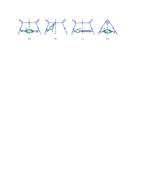
Representative diagrams for heavy-quark contributions in Eqs. (13) are shown in Fig. 1. The reader may consult this figure frequently to identify various terms in the ensuing discussion. Propagators and external legs for quarks that are indicated by thick lines (thin lines) will eventually be computed with full mass dependence (in the massless approximation) .
The heavy-quark diagrams fall into two categories, those that do not involve a collinear approximation for scattering of heavy quarks (often called “flavor-creation”, or FC, terms), and those that do (flavor-excitation, or FE, terms). While FC contributions must be evaluated exactly, the approximate nature of the FE terms allows some useful simplifications.
At , the flavor-creation contributions include the coefficients , , and . The heavy quarks appear in these terms inside the Feynman subgraph for , connected by a gluon propagator to an initial-state gluon or a light quark. These contributions are evaluated with the exact kinematical dependence on , and hence are defined unambiguously.
The FE cross sections are proportional to the heavy-quark PDF that approximates collinear production of heavy-quark pairs from light partons in the high-energy limit. Structure functions and coefficient functions with an initial-state heavy quark, such as and , fall into this class. The FE coefficient functions reduce to unique expressions when is negligible Collins (1998), but, near the threshold, they may differ by non-unique powerlike contributions with . Within the ACOT scheme, several conventions have been proposed to include the powerlike contributions in a way compatible with the QCD factorization theorem.222The differences between these conventions are formally of a higher order in , but some conventions lead to faster perturbative convergence.
Among these conventions, the “full ACOT scheme” Aivazis et al. (1994a) evaluates the FE coefficient functions ( etc.) with their complete mass dependence. The simplified ACOT (S-ACOT) scheme Collins (1998); Kramer et al. (2000) neglects all mass terms in and thereupon reduces tedious computations typical for the full ACOT scheme. The S-ACOT- scheme Tung et al. (2002) adopted in our computation includes the most important mass dependence in and uses simpler zero-mass expressions everywhere else. It generalizes the slow-rescaling prescription for single heavy quark production in neutrino DIS at leading order Barnett (1976) to other heavy final states and higher QCD orders.
If we use uppercase and lowercase letters to denote mass-dependent and massless quantities, and a caret to indicate renormalized ZM functions, the S-ACOT- convention for functions with initial-state heavy quarks can be summarized as
| (15) |
and
| (16) |
where
| (17) |
and is the net mass of all heavy particles produced in the final state. With the exception of a few very rare subprocesses identified below, at most one heavy-quark pair is produced in all cases that we consider. Without losing accuracy, we therefore assume throughout the computation.
This form is motivated by an observation that the largest powerlike terms are associated with the constraint imposed on the convolution by energy conservation in production of heavy final states Nadolsky and Tung (2009). The ZM functions here depend on the variable instead of Bjorken as an input parameter, and the momentum fraction in their convolutions is integrated over the range . The convention is justified in the context of the QCD factorization theorem in Sec. II.6. Its numerical impact is discussed in Sec. III.4.
When the S-ACOT- scheme is adopted, Eqs. (13) become
| (18) | |||
| (19) | |||
| (20) | |||
| (21) |
Lowercase functions in these equations are given by ZM expressions. Among all terms, only the structure functions and are calculated with the exact mass dependence. The carets above and indicate that the massless pole terms, and , have been subtracted from them.
In the rest of the terms, the input longitudinal variable is set to be . The convolution of such term with the PDF is
| (22) |
where . [The naive massless approximation is .]
The one-loop expressions , and can be found in Witten (1976); Aivazis et al. (1994a); Buza et al. (1998). and coincide with the massive structure functions with initial-state gluons and pure-singlet light quarks in Laenen et al. (1993); Riemersma et al. (1995). They are independent of . The expressions for and are computed as and in Buza et al. (1998).
The contribution corresponds to radiation of up to flavors of pairs off an incoming quark . It can be found as a sum of the pure-singlet and non-singlet ZM coefficient functions from Refs. Sanchez Guillen et al. (1991); van Neerven and Zijlstra (1991); Zijlstra and van Neerven (1991); Moch et al. (2005); Vermaseren et al. (2005):
| (23) |
In this equation, both pure-singlet and non-singlet parts of are taken to be massless, which is one of the choices possible within the S-ACOT scheme. Note that the functions with three indicated final-state (anti-)quarks and an unobserved fourth (anti-)quark among the target remnants could justifiably use a more restrictive rescaling variable, , as their parameter. Since their respective contributions are vanishingly small, it suffices to evaluate them with the same variable as in the rest of the terms to simplify the implementation.
It is equally acceptable to evaluate the pure-singlet with a massive subgraph, so that the corresponding coefficient function is given by the massive in Eq. (21). In this case, can be combined with the pure-singlet contribution with initial-state light quarks, also given by . The complete part of then takes a simple form
| (24) |
where is the singlet quark PDF summed over flavors:
| (25) |
We use Eq. (24) for practical implementation of , with the coefficient functions computed as in Eqs. (20) and (21).
II.3 Light-quark component of
By a similar argument, Eq. (7) serves as a starting point for finding coefficient functions for the light-quark component . The corresponding Wilson coefficients are
| (26) |
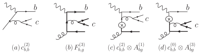
The quark-to-quark Wilson coefficients , and are decomposed into their PS and NS components as in Eq. (14). Non-singlet contributions and contain squared matrix elements with heavy-quark lines that are disconnected from the initial-state proton, as in Fig. 2. These diagrams must be evaluated with full dependence on . The rest of the coefficients in Eqs. (26) do not contain disconnected heavy-quark lines. They are computed according to ZM formulas.
Explicitly, the non-singlet functions with mass dependence consist of two parts, arising either from Feynman diagrams with light partons only (designated as ), or with a heavy quark in the final-state emission or virtual loop (denoted by ):
where or . The function , provided by the graphs of the type shown in Fig. 2, retains complete dependence. The function , obtained from the same graphs as in Fig. 2, but with the heavy quark replaced by one of the light quarks (), is evaluated in the ZM approximation.
Masses can be neglected in the rest of Eqs. (26), so we get
| (27) | |||
| (28) | |||
| (29) | |||
| (30) | |||
| (31) |
The one-loop coefficients have been known for a long time Bardeen et al. (1978); Altarelli et al. (1978); Humpert and van Neerven (1981). The two-loop massless contributions in Eqs. (30) and (31) can be derived from the published ZM results according to the following procedure. Using the decomposition Eq. (14) for in the ZM scheme,
| (32) |
where and are independent of the quark flavors or given that the masses are neglected, we write
| (33) |
with
The singlet PDF is given by Eq. (25), and the non-singlet sum of (anti-)quark PDFs is
Eq. (33) expresses in the same representation as Eq. (4.1) in the N3LO calculation of DIS cross sections Vermaseren et al. (2005). Comparing Eqs. (30) and (31) with ZM coefficient functions in Section 4 of that reference (which are indicated here by an asterisk ), we find that
| (34) |
| (35) |
and
| (36) |
with or for and respectively.
The non-singlet heavy-quark coefficient function,
| (37) |
is composed of contributions of several classes shown in Figs. 2(a)-(c). Diagrams with real emission of a heavy-quark pair (as in Fig. 2(a)) in contribute a function in Eqs. (A.1) and (A.2) of Ref. Buza et al. (1996). This contribution is combined with the virtual two-loop diagrams, cf. Fig. 2(b), to produce the first term on the right-hand side of Eq. (37), in which is regularized by the plus prescription at . Contributions with a heavy-quark polarization graph inserted into a one-loop scattering diagram, of the kind shown in Fig. 2(c), produce the second term in Eq. (37), where is available from Refs. Bardeen et al. (1978); Altarelli et al. (1978); Humpert and van Neerven (1981).
In this derivation, we do not explicitly compute the virtual loop contribution in Fig. 2(b), but deduce it from the Adler sum rule Adler (1966); Altarelli (1982); Dokshitzer et al. (1996); Brock et al. (1995). The sum rule states that the sum of the real and virtual contributions to satisfies
| (38) |
With this rule, it can be demonstrated that the virtual contribution amounts to imposing the plus prescription on as in Eq. (37).
In the asymptotic limit for the inclusive contains large terms proportional to . Those coincide with the non-singlet part of the light-quark PDF that arises from radiation of a heavy-quark pair as shown in Fig. 2(d). is computed as in Eq. (B.4) of Ref. Buza et al. (1998), which we evaluate as a function of in accord with the S-ACOT- scheme.
When is subtracted from as in Eq. (30), the difference is free of the collinear logs. After the difference is combined with the light-quark-only contributions , we obtain the full non-singlet coefficient function which coincides in the limit with its zero-mass expression in Eq. (8) of Ref. van Neerven and Zijlstra (1991). For the longitudinal function , the heavy-quark subtraction is zero. Putting everything together, we obtain the final expression for the NNLO light-quark component,
| (39) |
where the Wilson coefficients are listed in Eqs. (29)-(31) and (34)-(37).
II.4 Several heavy flavors
The structure functions and in Eqs. (39) and (24) are all that is needed to compute inclusive Our expressions can be readily extended to include two or more heavy-quark flavors:
| (40) |
where the sum runs over all quark flavors satisfying (i.e., up to the number of the kinematically allowed final-state flavors).
Beginning at , some contributions to include heavy quarks of two different flavors, say, and . For instance, Fig. 3(a) shows a two-loop diagram in in which an incoming bottom quark radiates a pair before or after the scattering on the photon. This flavor-excitation contribution, relevant at large enough, is evaluated by a massless expression, , in accord with the main rule of the S-ACOT scheme. We take the rescaling variable to be , given the numerical smallness of the cross section, even though a more restrictive choice conforms better with the exact momentum conservation in production of a + pair.
The above contribution resums the large- logarithmic behavior of a three-loop function for the process . A representative Feynman diagram is shown in Fig. 3(b). The rest of the diagrams in the class are related to the shown diagram by re-attaching the branch to one of the external legs (, , or ).
In the limit, simultaneously contains logarithms and that must be subtracted in order to obtain an infrared-safe coefficient function . The subtraction is realized by applying the perturbative expansion procedure discussed in Section II.2 to the three-loop level. We get
| (41) |
where the last two terms on the right-hand side are the subtractions associated with the diagrams of the type shown in Figs. 3(c) and (d). The functions , , and are evaluated with full dependence on and . [The coefficient has been recently computed in Ref. Ablinger et al. (2012).] The coefficient functions and are massless.
Based on the general structure of the S-ACOT scheme, we expect the first and third term in Fig. 3 to cancel when , and the fourth term to cancel the contribution to the term in the same limit. The third and fourth terms cancel the and contributions to the second term, , in the limit . The numerical realization of these cancellations at three loops is yet to be demonstrated in the future, pending on the calculation of the unknown massive three-loop coefficients. The factorization theorem is indicative of the structure of the S-ACOT- subtraction terms that will arise at that order.
II.5 Semi-inclusive heavy quark production
A clarification is needed that the heavy-quark component of inclusive (defined as the part proportional to the heavy-quark electric charge ) is not directly measurable. Rather, experiments publish the semi-inclusive (SI) heavy-quark structure function that is determined from the cross section with at least one registered heavy meson. In the case of at NNLO, with essentially coincides with the charm structure function that is commonly measured by HERA experiments.
While must be defined with care to obtain infrared-safe results at all Chuvakin et al. (2000), for a global fit it is sufficient to approximate in the following way Forte et al. (2010). At moderate values accessible at HERA, we define it as
| (42) |
Here is the component with the heavy quark struck by the photon, cf. Eqs. (12) and (24). , given by Eqs. (A.1) and (A.2) in Ref. Buza et al. (1996), is the non-singlet part of the light-quark component that contains radiation of a pair in the final state, as shown in Fig. 2(a). This is the same function that was discussed below Eq. (37). However, since the virtual diagram in Fig. 2(b) does not contribute to , the plus prescription is not imposed on in this case.
The function that is thus defined is numerically stable in comparisons to the existing data Forte et al. (2010). Our numerical analysis shows that the contribution associated with provides between 0 and 3% of the semi-inclusive charm cross sections at GeV, which is insignificant compared to typical experimental errors.
II.6 Factorization and convention
In the remainder of this section, we show that the S-ACOT- scheme is fully compatible with the QCD factorization theorem for DIS.
To see why the convention is needed, consider again the heavy-quark contribution to of the proton from Eq. (12),
| (43) |
This expression is for the same value as in Eq. (12), but the factorization scale GeV is taken to be below the switching-point scale for flavors, so that only PDFs for light parton flavors ) are present. For this scale choice, the PDFs do not include subgraphs with the heavy-quark lines: those are contained solely in the Wilson coefficient functions . The right-hand side is non-zero when the light parton carries enough energy to produce at least one pair in the final state. This condition is reflected in the integration limits that are imposed on the convolution by the energy conservation constraints inside the coefficient functions .
If is gradually increased above , a coefficient function with an initial-state heavy quark is introduced when crosses the switching point from to active flavors. This function does not automatically vanish outside of the physical range . If is defined so as to contribute in a wider range at the switching point, with , then the DGLAP evolution preserves the same wider range at all above the switching point.
If is the center-of-mass energy of the photon scattering on a light parton ,
| (44) |
a final state with several heavy particles of the net mass is produced when
| (45) |
According to this condition, the momentum fraction must be in the range
| (46) |
for production to occur, where .
If collinear approximations for flavor-excitation (FE) and subtraction terms in violate this fundamental requirement, large spurious contributions from the unphysical kinematical region cancel to each order of , but survive as higher-order logarithmic terms. They can be eliminated by a supplemental condition that the correct integration limits are always to be preserved, as in Eq. (46).333Even in the limit, convolutions with FE terms and subtractions could be in principle extended to include contributions from . This would not violate QCD factorization order by order, but will destabilize higher-order terms. This is avoided by an implicit assumption that the FE convolutions in the ZM limit are restricted to the physical range .
We will now show how to apply this condition at any order by including it into the QCD factorization theorem. For this purpose, we examine the projection operator that encapsulates the main rules of each factorization scheme Collins (1998). It applies a set of approximations to the Feynman graphs with leading momentum regions in order to enable all-order factorization.
We will closely follow the derivation and notations in Ref. Collins (1998). In this approach, the Feynman graphs containing the leading DIS contributions are composed of two-particle irreducible subgraphs and , joined by one parton line on each side of the unitarity cut. Each leading graph involves integration over the momentum of the intermediate parton and summation over its spin components,
| (47) |
Virtualities of all momenta are of order in the hard subgraph , and they are much smaller than in the target subgraph . eventually contributes to the Wilson coefficient functions, and to the PDFs. and are the photon’s and proton’s 4-momenta. The nearly massless proton moves in the direction in the Breit reference frame.
The purpose of the operator is to approximate the leading-power (logarithmically divergent) part of by a simpler expression, denoted by , and to recast as
| (48) |
The leading-power approximation provides the bulk of . The non-leading power part is suppressed by terms of order
When it is recursively applied to all leading subgraphs, the projection generates the factorized expression for the structure function, . Collins (1998)
The operation simplifies integration over the momentum and summation over the spin components of the intermediate parton, and it also simplifies the hard graph . The momentum of the parton that enters is replaced by a simpler momentum , e.g., if is massless (where ). The operation discards power-suppressed terms in , such as the masses of the light quarks that are always negligible compared to . It also specifies when the heavy-quark mass terms are to be retained in , depending on the type of the factorization scheme and the partonic scattering subprocess.
In all variants of the ACOT scheme, the operator is the same in all partonic channels except for the subgraphs with an incoming heavy-quark line. The target parts , operators and for the subgraphs with initial light-quark and gluon lines are identical in all variants, while the operator for the subgraphs with incoming heavy quarks is not. The PDFs in are defined by the operator matrix elements as in Eq. (3) and retain dependence on quark masses of all contributing flavors.
The operator is of the form
where and are projectors on the leading spin components in and , respectively. The incoming heavy quark in has an approximate momentum where the light-cone components of in the Breit frame are and . With this representation, the integral assumes the form of a convolution over ,
| (49) |
where is the ratio of the large “+” momentum components.
| Scheme | in | in | range in | |
|---|---|---|---|---|
| ACOT | ||||
| S-ACOT | ||||
| S-ACOT- |
Table 1 collects expressions for and in the ACOT, S-ACOT, and S-ACOT- schemes. It also lists the integration ranges in the convolutions and indicates if is set to zero in the subgraphs. We re-emphasize that the three schemes listed in the table are distinguished only by the hard subgraphs, or Wilson coefficients, with initial-state heavy quarks, i.e., in the flavor-excitation channel. The differences arise solely in the terms proportional to powers of in . One could simplify the FE hard-scattering contributions by setting as in the S-ACOT scheme. In the full ACOT scheme, the lower limit of integration in is set by the kinematics of scattering of a massive quark into a massive quark, which violates the momentum conservation condition of Eq. (43) for pair production of massive quarks from light-quark scattering. In the S-ACOT scheme, one is tempted to set the integration range to which is also incompatible with momentum conservation. One cannot just restrict the integration range to as this disallows the lowest-order FE contribution that contributes at .
A better way is provided by the rescaling , which leaves invariant, as it does not change , , or other kinematical variables in . At the same time, rescaling changes the integration range for in the convolution.
Choosing we obtain the S-ACOT- scheme that has all desirable features:
- 1.
-
2.
The integration over proceeds over the physical range in all channels. It includes all physically possible scattering channels for , but excludes kinematically prohibited values for . Since the form of is associated with a specific coefficient function, the same form is to be used in convolutions of this coefficient function in subtraction terms at higher orders.
-
3.
The S-ACOT- coefficient functions in the flavor-excitation channels are given by ZM expressions evaluated at . Kinematical prefactors outside of the coefficient functions are independent of and not affected by the rescaling.
-
4.
The target subgraphs , corresponding to the PDFs, are given by universal operator matrix elements that are the same in all ACOT-like schemes.
-
5.
The same value is used in the evolution of , PDFs, and hard graphs in each range.
-
6.
When is much larger than the coefficient functions of the S-ACOT- scheme reduce to those of the zero-mass scheme, without additional finite renormalizations.
-
7.
When is of order , the S-ACOT- scheme is generally closer to the FFN scheme than the S-ACOT scheme as a consequence of its operation that satisfies energy conservation. In this scheme, matching onto the FFN scheme does not rely on propositions beyond the factorization theorem with energy conservation, such as conditions for derivatives of Thorne and Roberts (1998b) or damping factors Forte et al. (2010).
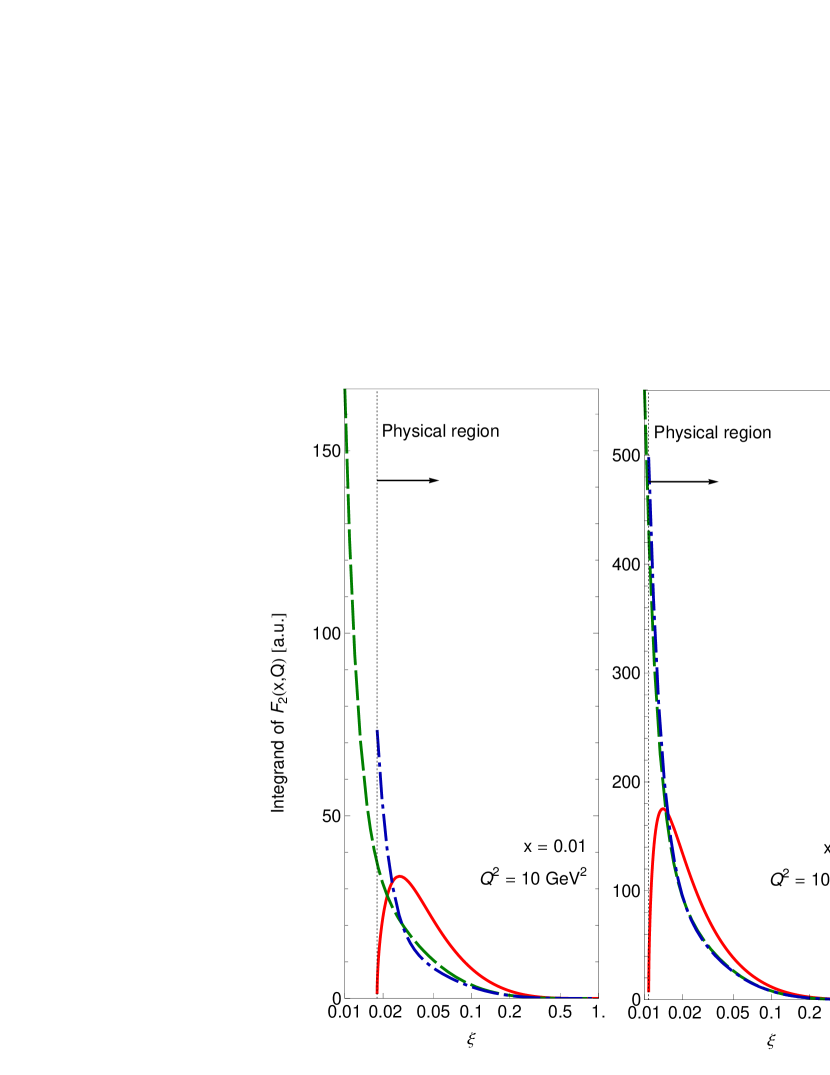
An illustration for the convention
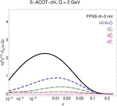
The advantages of rescaling can be demonstrated on the example of the contribution, consisting of the gluon-initiated box graph and corresponding subtraction, and shown by the second and third graphs on the upper row of Fig. 1:
| (50) |
The integrands of the convolution integrals on the right-hand side, and , where or are plotted in Fig. 4(a-c) as a function of . The computation follows the numerical setup described in the next section. The scale on the axis is logarithmic: the convolution integrals are proportional to the areas under the respective integrand curves. For definiteness, we choose and 10, 100, and 10000 , but the same features are observed for other and values.
In the charm creation contribution, , the integrand (red solid line) vanishes outside of the physical range , where and for 10, 100, and 10000 . On the other hand, the naive choice of the S-ACOT scheme allows the integrand (green dashed curve) in the second term on the right-hand side of Eq. (50) to contribute in the unphysical region . Its spurious contribution is comparatively large at the smallest . It is not fully canceled by the counterpart FE term in the first upper graph of Fig. 1, leading to a bloated higher-order uncertainty.
The S-ACOT- integrand vanishes below (cf. the blue dash-dotted line). It is numerically moderate at physical values, , and its integral cancels well with , as will be further demonstrated in Sec. IV.1. Note also that the difference between the two definitions for the integrand is small in most of the physical range
As the virtuality increases, the difference between and progressively reduces, and varies in a wider interval. Finally in (c), for very large , the S-ACOT and S-ACOT- subtractions become identical. approximates well the collinear splitting contribution that drives much of the shape of . When is subtracted from as in Eq. (50), it produces a moderate negative contribution, which is further reduced at NNLO. These cancellations are further examined in Sec. IV.2.
III Numerical examples
In this section, we show representative plots from our validation tests for the NNLO inclusive structure functions and computed according to the S-ACOT- scheme. We focus on the partial contributions in which the photon strikes a charm quark, given by in Eq. (12) for , and for structure functions or . These contributions are referred to as and in the figures. The same comparisons have been repeated for the bottom-quark functions and as well as for the full inclusive functions and alternative values of Bjorken The results of other tests show similar patterns and can be viewed at Guzzi and Nadolsky (2010).
NNLO coefficient functions for massive quarks are computed using a program available from Riemersma et al. (1995). This program tabulates two-loop heavy-quark coefficient functions in a form that allows fast evaluation of convolution integrals in the range covered by the experimental data.
The PDFs in all comparisons are obtained by using the Les Houches Accord toy parametrization Giele et al. (2002); Whalley et al. (2005) at the starting scale GeV. Other input parameters are and the pole mass .444Our program can alternatively read masses as the input. In this case, the masses are later converted into the respective pole masses, because the operator matrix elements are published as functions of the pole masses. The switching between 3 and 4 flavors happens at . The and PDFs are evolved to higher values by the HOPPET computer code Salam and Rojo (2009).555Bottom-quark contributions are omitted in this comparison. The charm PDF is zero at , but acquires a non-negligible value immediately above through an discontinuity existing at the switching point.
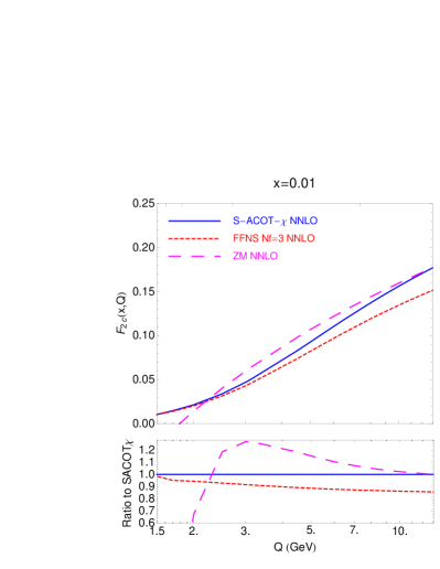
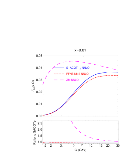
III.1 dependence
Fig. 5 examines dependence of charm structure functions (left panel) and (right panel). They are computed to order in all schemes, referred to as “NNLO” by the counting convention for the inclusive structure functions considered here. [In predictions for semi-inclusive charm production, the cross section in the FFN scheme is often counted as NLO, since the flavor-excitation cross section is absent in this scheme.] The upper insets in both panels show predictions at in the S-ACOT- scheme, FFN scheme with , and ZM scheme with . The lower insets show ratios of the FFN and ZM predictions to the S-ACOT- prediction.
The left panel shows that the S-ACOT- theory prediction for (blue solid line) is numerically close to the FFN prediction (red short-dashed line) at and to the ZM prediction (magenta long-dashed line) at GeV.
Similarly, in the right panel, the S-ACOT- prediction for the longitudinal function coincides with the corresponding FFN prediction at and approaches the ZM prediction at GeV. [ is sensitive to mass-dependent corrections to scattering off longitudinally polarized photons. Its matching on the ZM prediction happens at higher values than in .] The S-ACOT- prediction interpolates between the FFN and ZM predictions at intermediate values, precisely as expected.
III.2 Dependence on the factorization scale
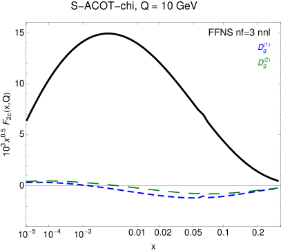
(a) (b)
(c) (d)
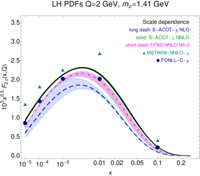
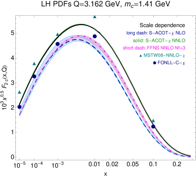
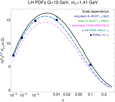
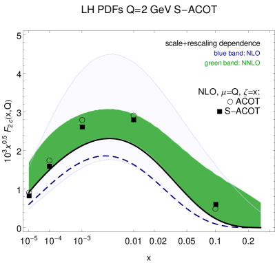
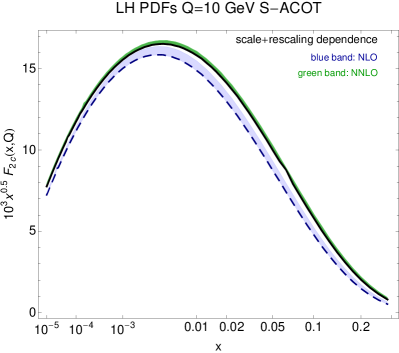
NLO computations leave substantial uncertainty in the DIS charm-quark contributions due to the choice of the renormalization/factorization scale and differences in the FE terms in the threshold region. NNLO terms drastically reduce these uncertainties. Factorization scale dependence, and its reduction from NLO to NNLO, is illustrated by Fig. 6. Reduction of uncertainties in the modeling of kinematical threshold effects is discussed in Sec. III.4.
In Fig. 6(a)-(c), predictions for in the S-ACOT- and FFN () schemes are plotted versus Bjorken at representative values of 4, 10, and 100 . The values on the axis are multiplied by to better visualize the accessible region. Central predictions are computed for , the default scale in heavy-quark DIS cross sections in the CT10 global analysis Lai et al. (2010). The error bands are obtained by varying the scale in the range .
At GeV in Fig. 6(a), the NNLO S-ACOT- central prediction (black solid line inside a green band) is slightly above the NNLO FFN prediction (short-dashed line inside a magenta band) and has a smaller scale uncertainty than FFN. At below 2 GeV (not shown), the NNLO S-ACOT- and FFN predictions get even closer. In contrast, the NLO S-ACOT- prediction (a long-dashed line inside a blue band) underestimates the NNLO FFN result and has wider scale dependence.
As increases to 10 GeV (Fig. 6(c)), S-ACOT- predicts more event rate than the FFN scheme both at NLO and NNLO. Altogether, the dependence in these figures is fully compatible with the matching of the S-ACOT- results on the FFN and ZM results in the limits and , respectively.
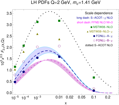
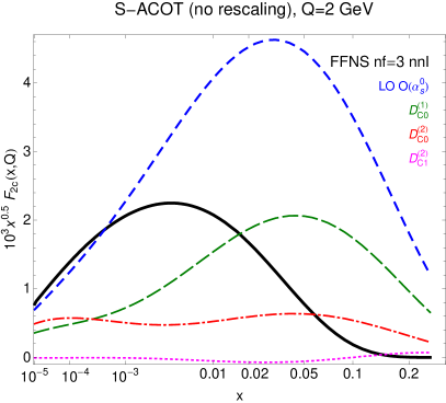
III.3 NNLO vs. NLO predictions
Improved stability of the NNLO prediction in Fig. 6(a) can be appreciated by comparing it to the counterpart NLO result shown in Fig. 6(d). Here, we collect NLO values at GeV, obtained in the FFN and S-ACOT schemes. We also show NLO predictions in the modified Thorne-Roberts (TR’) scheme Thorne and Roberts (1998b, a); Thorne (2006)), as implemented by the MSTW’08 PDF analysis Martin et al. (2009), and in the FONLL schemes A and B used by the NNPDF collaboration Forte et al. (2010). The S-ACOT and MSTW predictions are shown with the scaling as well as without it.
The spread in NLO values of observed in the figure is extensive, nominally suggesting a large uncertainty in the resulting NLO PDF sets. However, when included in the PDF fits, the most extreme predictions for in this figure are excluded by the fitted DIS data, which prefer the values that are about the same as the (relatively unambiguous) NNLO result. In the CT10 NLO fit, the scale is set equal to , which brings the NLO S-ACOT- prediction in agreement with the measured cross sections. Thus, according to the past global fits, the NLO cross sections can be reconciled with the heavy-quark data, but at the expense of tuning of the scale parameter, for each value of and rescaling variable. The key benefit of the NNLO calculation for is to automatically achieve such a good agreement, nearly independently of the factorization scale.
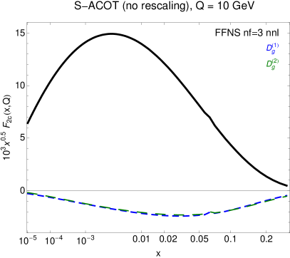
III.4 Threshold effects
(a) (b)
In the above discussion, our NNLO structure functions are computed using the optimal rescaling variable in the FE heavy-quark contributions. The rescaling variable significantly improves convergence near the threshold by excluding contributions to the FE convolution integrals that are kinematically disallowed.
Dependence on the rescaling prescription can be explored with the help of the variable that generalizes the variable as proposed in Ref. Nadolsky and Tung (2009). The generalized rescaling variable is implicitly defined by
| (51) |
where is a real number. Various choices of positive produce a family of GM schemes in which takes continuous values between (no rescaling) and (full rescaling). Specifically, produces of the S-ACOT- scheme, and produces that corresponds to the plain S-ACOT scheme without rescaling. Negative values (not shown) strongly suppress the FE contributions by setting .
Fig. 7 shows the bands of variations in the NLO and NNLO S-ACOT values at GeV (left panel) and 10 GeV (right panel) when and are varied in the ranges and , respectively. If is naively varied in the full range, at smallest values one obtains a large excursion in the NLO predictions (light blue band), which is considerably reduced when going to NNLO (green band).
The ACOT and S-ACOT schemes without rescaling (corresponding to ) are less motivated than the S-ACOT- scheme, since they include kinematically disallowed small- contributions that destabilize perturbation theory. To give an idea about these less favored schemes, the upper boundary of the green band in Fig. 7 corresponds to the NNLO S-ACOT calculation (without rescaling) for the scale . Lower values of the scale, such as , reduce the S-ACOT cross section and bring it closer to the S-ACOT- cross section for (the black solid line). [The scale dependence of the S-ACOT cross section is larger than that of the S-ACOT- cross section.]
The distinction between the ACOT and S-ACOT schemes arises from the additional “dynamic” mass terms in the ACOT flavor-excitation Wilson coefficients, which have little numerical effect Kramer et al. (2000). An NNLO calculation in the full ACOT scheme is difficult and was not completed, but already at NLO the ACOT and S-ACOT schemes become very close. The left panel compares the NLO values in the ACOT and S-ACOT schemes for without rescaling from Ref. Rojo et al. (2010), as indicated by the circles and squares, respectively. The discrepancy between the ACOT and S-ACOT values is small already at NLO. It is likely to further decrease when going to the NNLO as a term of order .
As increases above a few GeV, dependence on diminishes practically to nil, as in the right panel of the figure for GeV. The ACOT and S-ACOT scheme produce essentially coinciding predictions at such a large value Rojo et al. (2010). Together with Fig. 6, Fig. 7 indicates that, at NNLO, the physically motivated rescaling variable is more important at low than the factorization scale choice or the difference between the ACOT and S-ACOT schemes.
III.5 Alternative mass schemes
III.5.1 TR’ and FONLL schemes
Figs. 6(a)-(c) also show NNLO predictions in the alternative GM schemes, indicated by scattered symbols: the modified Thorne-Roberts (TR’) scheme and FONLL scheme C. Their values are computed in the 2009 Les Houches benchmark study of GM schemes Rojo et al. (2010) by assuming the same rescaling as the S-ACOT- scheme.
The three schemes are seen to be in good overall agreement, apart from minor differences traced to subtle variations in the NNLO implementations that the schemes provide.
At GeV, the NNLO S-ACOT- prediction lies slightly above the FONLL-C prediction and below the MSTW prediction. At GeV, the NNLO S-ACOT- prediction becomes closer to the MSTW prediction and is still above the FONLL-C result. These differences can be understood by noticing that the compared schemes may differ in subleading perturbative terms. For example, the FONLL-C scheme includes a threshold damping factor to match on the 3-flavor result near the threshold Forte et al. (2010). The S-ACOT- scheme is not using the damping factor and is expectedly close to the FONLL-C scheme at , but not strictly identical. The TR’/MSTW prediction includes a constant higher-order term (of order ) to improve smoothness of switching from 3 to 4 active flavors at . Neither S-ACOT- nor FONLL-C include this artificial constant term, which is why they may predict smaller values at low .
III.5.2 The BMSN scheme
Structural similarities between the S-ACOT-, TR’, and FONLL schemes reflect their conceptual origin from the Collins-Wilczek-Zee (CWZ) renormalization method Collins et al. (1978). The CWZ procedure is applied frequently to renormalize QCD quantities dependent on several mass scales. It introduces a sequence of renormalization schemes and associated differential equations that operate with the number of active flavors that changes across the particle mass thresholds. The CWZ procedure is invoked, for example, in the common definition of the QCD running coupling and by the zero-mass VFN scheme.
The family trait of the CWZ renormalization – a hierarchy of fixed-flavor number subschemes with sequentially incrementing values – is also present in the ACOT-like general mass schemes. In practical realizations of these schemes, scale dependence of both and PDFs is found by solving renormalization group equations with a shared value in each mass range. The and expressions for and PDFs are related at the switching momentum scales through the known matching conditions.
A different path is taken in the approach of Buza, Matiuonine, Smith, and van Neerven (BMSN Buza et al. (1998)), which is adopted in the fits by the ABM group Alekhin et al. (2010, 2012). In the BMSN and CSN Chuvakin et al. (2000) frameworks, only is found from a renormalization group equation according to the CWZ procedure. However the 4-flavor PDFs are constructed from the -flavor PDFs at by solving the matching equations for each value. Only the -flavor PDFs are evolved by the DGLAP equations in this case. Here we see the key difference with the ACOT approach, which resums higher-order corrections to the heavy-flavor PDFs at with the help of DGLAP equations. The BMSN method does not provide this resummation, crucial for implementing the collider data from into the global fit. To resum the heavy-quark collinear logs in their published 5-flavor PDFs, ABM evolve them from the initial scale to higher energies after the fit, starting from the best-fit parametrization found in the BMSN approach.
In the BMSN framework, the number of active quark flavors in is incremented from 3 to 5 according to the usual convention as the energy increases. -flavor PDFs are derived from the -flavor PDFs as
| (52) |
The functions are comprised of the coefficients in the perturbative expansion of the massive parton-level PDFs that were discussed in Sec. II.1. The BMSN 4-flavor structure function is given by
| (53) |
where is obtained for three massless quarks ( ) and one massive quark (). is the dominant part of in the asymptotic limit , and is computed with 4 massless quarks in the Wilson coefficients, with the 4-flavor PDFs defined by Eq. (52).
This arrangement provides a nearly ideal matching of the -flavor onto the 3-flavor as , possible only in the absence of resummation of collinear logs . At , the last two terms in Eq. (53) are related by the replacement of the 3-flavor QCD coupling by the 4-flavor coupling,
| (54) |
Since is nearly continuous at the switching point between 3 and 4 flavors (apart from a mild discontinuity that first enters at ), it follows from Eqs. (53) and (54) that at . The matching onto the FFN scheme at is achieved by dropping numerical DGLAP evolution of 4-flavor PDFs.
In deriving these relations, BMSN allow only one parton flavor to be massive in each range. This assumption is untrue at some level for comparable to , since is not negligible compared to It creates conceptual difficulties in extending the VFN scheme proposed by BMSN to three loops Ablinger et al. (2011b); Ablinger et al. (2012), since both the parton-level structure functions and operator matrix elements may depend on and at the same time.
In fact, this assumption is not necessary for proving QCD factorization with heavy quarks and is not made in the S-ACOT approach. The proof of the general-mass factorization scheme does not assume that all quarks but one are massless. Masses of heavy quarks that may be comparable to are never neglected in the target subgraphs associated with the PDFs and , cf. Ref. Collins (1998) and Sec. II.6. As an illustration of their role, consider again the coefficient function with and quark lines in Eq. (41) of Sec. II.4. This function is found by subtracting convolutions of massive operator matrix elements from a massive parton-level function . This is expected to produce that is free of the and terms and coincides with in the effective scheme with 5 massless flavors when is unequivocally larger than and . [Verification of this prediction still awaits an explicit calculation of the massive function ]. The operator matrix element that depends both on and , and which caused concern in Refs. Ablinger et al. (2011b); Ablinger et al. (2012), therefore naturally appears in the factorization formula (41) when deriving the infrared-safe with two quark species. It is not anticipated to pose a problem from the S-ACOT- viewpoint.
Numerically, the S-ACOT- and BMSN approaches provide close predictions for charm production at Rojo et al. (2010). While both approaches are in good agreement with the current HERA data, they may lead to numerical differences in future precise DIS analyses, both at scales of order where the resummed terms may already play some role, and at electroweak scales, where the expected differences of a few percent may be comparable to the PDF uncertainties. More generally, S-ACOT- points out a way to include heavy-quark mass dependence and resummation of heavy-quark collinear logs in one step, and to implement three-loop DIS amplitudes with two massive quark flavors along the guidelines of the CWZ renormalization.
IV Cancellations between Feynman graphs
IV.1 Cancellations at low
In order to match on the FFN and ZM predictions, certain classes of Feynman diagrams inside the S-ACOT- NNLO coefficient functions must cancel in the respective low- and large- regions. We will show how these cancellations come about in the case of the charm-quark function , but the pattern holds for the bottom quark and other structure functions with suitable modifications.
The cancellations are revealed by plotting differences between various matrix elements and collinear subtractions discussed in Section II.1, which are established by applying the factorization formula at the parton level.
In the region, all FE contributions in Eqs. (18)-(21) must cancel to a high degree in order for to reduce to the FFN matrix elements and . In the threshold region, the evolved charm PDF is effectively of order ,
| (55) |
a FE contribution to containing a coefficient is effectively of order ) . Keeping this in mind, at order the virtual-photon-charm scattering diagram with in Eq. (18) cancels the gluon-initiated subtraction term with in Eq. (19), and only the fusion diagram in Eq. (19) survives in the total In this case, the difference
| (56) |
where and represent the charm and gluon PDFs, must be close to zero.
As the next order is included, the cancellation present in must further improve. Two differences quantify the cancellations to this order:
| (57) |
in which the convolutions of with operator matrix elements and are subtracted from ; and
| (58) |
which probes the cancellation between convolutions involving the coefficient . By comparing with , we quantify how the cancellation in , proportional to improves upon the inclusion of the NNLO corrections. The difference quantifies yet another cancellation that is independent of . It has the same structure as , but includes the convolutions with instead of .
The left panel of Fig. 8 shows the dependence of , , and at GeV. To provide visual guidance, these differences are compared to the FFN prediction at (solid black line), which is roughly equal to the total rate at this (cf. the previous subsection). We also plot the S-ACOT- contribution of provided by (dashed blue line), nominally counted as the lowest-order contribution. While the LO contribution on its own is substantial comparatively to the FFN result, it is mostly canceled by the subtraction in Eq. (56), so that the resulting difference (long-dashed green line) is small.
The cancellation in is further improved by including the next-order terms in as in Eq. (57). The difference (dot-dashed red line) and especially the counterpart difference (dotted purple line) give decreasingly small contributions. They satisfy
| (59) |
Therefore, as , the S-ACOT- scheme exhibits an almost perfect match on the FFN computation by the virtue of perturbative cancellations that improve with each order of .
IV.2 Cancellations at large
A different cancellation pattern is observed when is negligible compared to , when the large logarithms collected in , etc. must be subtracted from the massive contributions to obtain the infrared-safe coefficient functions . These cancellations are illustrated in the right panel of Fig. 8 by and . They quantify the collinear subtractions in the contributions containing the box subgraph. The lowest-order difference is equal to the convolution of the coefficient as defined by Eq.(19):
| (60) |
In this expression the subtraction term matches on the photon-gluon contribution represented by . The dependence of this matching is shown in the right panel of Fig. 8 for GeV. It can be seen that (blue short-dashed line) is quite small compared to the FFN result.
The -order difference can be constructed as
which can be cast into the form
| (61) |
by virtue of Eqs. (20) and (21). At this order, the collinear logarithms arising in are canceled by and , and, similarly, the collinear term in is removed by . The net effect of the subtractions is that (the green long-dashed line) provides a small correction to . The perturbative series converge well for :
| (62) |
IV.3 Cancellations without kinematic rescaling
Although the cancellations happen for any rescaling variable , their perturbative convergence is slower for a non-optimal choice, such as . The differences etc. for are shown in Fig. 9 and, as one can see, they are generally larger than in the case of Nonetheless, the differences are reduced by going to NNLO, although not as fast as for the optimal rescaling choice.
V Conclusions
We examined connections between multi-loop calculations for massive quark production and fundamental concepts behind QCD factorization. An NNLO calculation for neutral-current DIS with massive quarks is documented in a form that bears structural similarity to the NNLO computation in the zero-mass scheme Sanchez Guillen et al. (1991); van Neerven and Zijlstra (1991); Zijlstra and van Neerven (1991). This calculation is algorithmic and utilizes readily available NNLO expressions. The main formulas are presented by Eqs. (40), (24), and (39). The theoretical derivation presented in Sec. II can be readily extended to two loops in charged-current DIS, after all needed heavy-quark matrix elements are computed.
The conceptual foundation for the presented results is provided by the S-ACOT- factorization scheme. The discussion emphasized several strong features of this scheme: its direct origin from the proof of QCD factorization for DIS Collins (1998), relative simplicity, and compliance with phase space constraints on heavy-quark production at all energies.
Throughout this study, we highlighted phenomenological importance of energy conservation in massive particle production. We have shown how the constraints from energy conservation can be satisfied in all channels as a part of the QCD factorization theorem. These constraints are included in the definition of the operation in the Collins’ proof of QCD factorization by rescaling the partonic momentum fraction in flavor-excitation Wilson coefficients. The rescaling variable depends on the mass of heavy particles in the final state as , where = and at the lowest order in neutral-current DIS and charged-current DIS, respectively. The S-ACOT- scheme thus realizes correct kinematical dependence solely by the means of the QCD factorization theorem and momentum conservation.
Schemes of the ACOT family differ only in mass-dependent terms in heavy-quark Wilson coefficient functions. PDFs are given by the same operator matrix elements in all schemes, such as Eq. (3). Estimates of these PDFs from global fits converge to unique universal functions as order of the QCD coupling increases. Convergence is the fastest in the S-ACOT- scheme.
At NNLO, dependence of S-ACOT- predictions on the factorization scale and other tunable parameters is reduced compared to NLO. Cancellations between classes of Feynman diagrams are stabilized once NNLO terms are included.
After the first version of this paper has been submitted, an independent S-ACOT- calculation for NC DIS has been realized in Ref. Stavreva et al. (2012). In that approach, full mass dependence is included at , while approximate matrix elements are used in all heavy-quark channels at and . They are obtained from ZM matrix elements evaluated with a rescaling variable that mimic the dominant kinematic contributions, in an approach that resembles the “intermediate-mass” scheme proposed in Ref. Nadolsky and Tung (2009). In our study, the contributions to flavor-creation channels and threshold matching coefficients are computed exactly, so that it reduces to the FFN scheme at . Since the kinematical mass terms dominate over the dynamical terms in most practical situations Nadolsky and Tung (2009), the calculation in Ref. Stavreva et al. (2012) is beneficial for obtaining estimates of yet unknown heavy-quark coefficient functions, notably for heavy-quark contributions to neutral-current DIS at three loops and charged-current DIS at two loops.
The derivation of S-ACOT- predictions is simpler than in some other GM schemes Buza et al. (1998, 1997), as it is carried out by assuming a unique number of active flavors () and one set of universal PDFs in every range. It is minimal, in the sense that it does not impose conditions on the derivatives of structure functions Thorne and Roberts (1998a) or introduce a damping factor Forte et al. (2010). Yet, after the NNLO terms are included, the S-ACOT- predictions result in good agreement with the other GM schemes. As the default heavy-quark scheme of CTEQ PDF analyses, the S-ACOT- scheme is going to play a crucial role in global fits at NNLO.
Acknowledgments
Many ideas in this paper were inspired by Wu-Ki Tung. We thank J. Smith for providing the computer code for computing massive NNLO DIS cross sections and for helpful comments on this work. We benefited from discussions with J. Huston, F. Olness, J. Pumplin, D. Stump, and other CTEQ members. M.G. and P.M.N. appreciate stimulating communications with S. Alekhin, J. Blümlein, A. Cooper-Sarkar, S. Forte, A. Mitov, S. Moch, J. Rojo, and R. Thorne. This work was supported in part by the U.S. DOE Early Career Research Award DE-SC0003870; by the U.S. National Science Foundation under grant PHY-0855561; by the National Science Council of Taiwan under grants NSC-98-2112-M-133-002-MY3 and NSC-99-2918-I-133-001; and by Lightner-Sams Foundation. CPY appreciates hospitality of the National Center for Theoretical Sciences in Taiwan, where a part of this work was done. MG thanks the hospitality of DESY during the work on the updated version.
References
- Tung et al. (2007) W. K. Tung et al., JHEP 02, 053 (2007).
- Aivazis et al. (1994a) M. A. G. Aivazis, J. C. Collins, F. I. Olness, and W.-K. Tung, Phys. Rev. D50, 3102 (1994a).
- Collins (1998) J. C. Collins, Phys. Rev. D58, 094002 (1998).
- Kramer et al. (2000) M. Kramer, 1, F. I. Olness, and D. E. Soper, Phys. Rev. D62, 096007 (2000).
- Tung et al. (2002) W.-K. Tung, S. Kretzer, and C. Schmidt, J. Phys. G28, 983 (2002).
- Lai et al. (2010) H.-L. Lai et al., Phys. Rev. D82, 074024 (2010).
- Nadolsky et al. (2008) P. M. Nadolsky et al., Phys. Rev. D78, 013004 (2008).
- Pumplin et al. (2009) J. Pumplin et al., Phys. Rev. D80, 014019 (2009).
- Moch and Rogal (2007) S. Moch and M. Rogal, Nucl.Phys. B782, 51 (2007).
- Moch et al. (2009) S. Moch, J. Vermaseren, and A. Vogt, Nucl.Phys. B813, 220 (2009).
- Buza and van Neerven (1997) M. Buza and W. van Neerven, Nucl.Phys. B500, 301 (1997).
- Buza et al. (1998) M. Buza, Y. Matiounine, J. Smith, and W. L. van Neerven, Eur. Phys. J. C1, 301 (1998).
- Chuvakin et al. (2000) A. Chuvakin, J. Smith, and W. L. van Neerven, Phys. Rev. D61, 096004 (2000).
- Thorne and Roberts (1998a) R. S. Thorne and R. G. Roberts, Phys. Lett. B421, 303 (1998a).
- Thorne and Roberts (1998b) R. S. Thorne and R. G. Roberts, Phys. Rev. D57, 6871 (1998b).
- Thorne (2006) R. S. Thorne, Phys. Rev. D73, 054019 (2006).
- Alekhin et al. (2010) S. Alekhin, J. Blümlein, S. Klein, and S. Moch, Phys. Rev. D81, 014032 (2010).
- Forte et al. (2010) S. Forte, E. Laenen, P. Nason, and J. Rojo, Nucl. Phys. B834, 116 (2010).
- Sanchez Guillen et al. (1991) J. Sanchez Guillen, J. Miramontes, M. Miramontes, G. Parente, and O. A. Sampayo, Nucl. Phys. B353, 337 (1991).
- van Neerven and Zijlstra (1991) W. L. van Neerven and E. B. Zijlstra, Phys. Lett. B272, 127 (1991).
- Zijlstra and van Neerven (1991) E. B. Zijlstra and W. L. van Neerven, Phys. Lett. B273, 476 (1991).
- Thorne (2010) R. Thorne, PoS DIS2010, 053 (2010), eprint 1006.5925.
- Alekhin et al. (2011) S. Alekhin, S. Alioli, R. D. Ball, V. Bertone, J. Blümlein, et al. (2011), eprint arXiv:1101.0536.
- Plačakytė (2010) R. Plačakytė (2010), talk at the PDF4LHC meeting, http://indico.cern.ch/materialDisplay.py?contribId=6&sessionId=2&materialId=slides&confId=103872.
- Aaron et al. (2010) F. Aaron et al. (H1 and ZEUS Collaboration), JHEP 1001, 109 (2010).
- Laenen et al. (1993) E. Laenen, S. Riemersma, J. Smith, and W. L. van Neerven, Nucl. Phys. B392, 162 (1993).
- Riemersma et al. (1995) S. Riemersma, J. Smith, and W. L. van Neerven, Phys. Lett. B347, 143 (1995).
- Harris and Smith (1995) B. Harris and J. Smith, Nucl.Phys. B452, 109 (1995).
- Buza et al. (1997) M. Buza, Y. Matiounine, J. Smith, and W. van Neerven, Phys.Lett. B411, 211 (1997).
- Bierenbaum et al. (2007) I. Bierenbaum, J. Blümlein, and S. Klein, Nucl.Phys. B780, 40 (2007).
- Bierenbaum et al. (2009a) I. Bierenbaum, J. Blümlein, and S. Klein, Phys.Lett. B672, 401 (2009a).
- Blümlein et al. (2006) J. Blümlein, A. De Freitas, W. van Neerven, and S. Klein, Nucl.Phys. B755, 272 (2006).
- Bierenbaum et al. (2009b) I. Bierenbaum, J. Blümlein, and S. Klein, Nucl.Phys. B820, 417 (2009b).
- Ablinger et al. (2011a) J. Ablinger, J. Blümlein, S. Klein, C. Schneider, and F. Wissbrock, Nucl.Phys. B844, 26 (2011a).
- Blümlein et al. (2012) J. Blümlein, A. Hasselhuhn, S. Klein, and C. Schneider (2012), eprint arXiv:1205.4184.
- Ablinger et al. (2011b) J. Ablinger, J. Blümlein, S. Klein, C. Schneider, and F. Wissbrock (2011b), eprint arXiv:1106.5937.
- Ablinger et al. (2012) J. Ablinger, J. Blümlein, A. Hasselhuhn, S. Klein, C. Schneider, et al. (2012), eprint arXiv:1202.2700.
- Laenen and Moch (1999) E. Laenen and S.-O. Moch, Phys.Rev. D59, 034027 (1999).
- Kawamura et al. (2012) H. Kawamura, N. L. Presti, S. Moch, and A. Vogt (2012), eprint arXiv:1205.5727.
- Aivazis et al. (1994b) M. A. G. Aivazis, F. I. Olness, and W.-K. Tung, Phys. Rev. D50, 3085 (1994b).
- Barnett (1976) R. M. Barnett, Phys.Rev.Lett. 36, 1163 (1976).
- Nadolsky and Tung (2009) P. M. Nadolsky and W.-K. Tung, Phys. Rev. D79, 113014 (2009).
- Witten (1976) E. Witten, Nucl. Phys. B104, 445 (1976).
- Moch et al. (2005) S. Moch, J. A. M. Vermaseren, and A. Vogt, Phys. Lett. B606, 123 (2005).
- Vermaseren et al. (2005) J. Vermaseren, A. Vogt, and S. Moch, Nucl.Phys. B724, 3 (2005).
- Bardeen et al. (1978) W. A. Bardeen, A. J. Buras, D. W. Duke, and T. Muta, Phys. Rev. D18, 3998 (1978).
- Altarelli et al. (1978) G. Altarelli, R. K. Ellis, and G. Martinelli, Nucl. Phys. B143, 521 (1978).
- Humpert and van Neerven (1981) B. Humpert and W. L. van Neerven, Nucl. Phys. B184, 225 (1981).
- Buza et al. (1996) M. Buza, Y. Matiounine, J. Smith, R. Migneron, and W. van Neerven, Nucl.Phys. B472, 611 (1996).
- Adler (1966) S. L. Adler, Phys. Rev. 143, 1144 (1966).
- Altarelli (1982) G. Altarelli, Phys. Rept. 81, 1 (1982).
- Dokshitzer et al. (1996) Y. L. Dokshitzer, G. Marchesini, and B. R. Webber, Nucl. Phys. B469, 93 (1996).
- Brock et al. (1995) R. Brock et al. (CTEQ), Rev. Mod. Phys. 67, 157 (1995).
- Guzzi and Nadolsky (2010) M. Guzzi and P. Nadolsky (2010), http://hep.pa.msu.edu/cteq/public/SACOTNNLO2011/.
- Giele et al. (2002) W. Giele et al. (2002), eprint hep-ph/0204316.
- Whalley et al. (2005) M. R. Whalley, D. Bourilkov, and R. C. Group (2005), eprint hep-ph/0508110; http://hepforge.cedar.ac.uk/lhapdf/.
- Salam and Rojo (2009) G. P. Salam and J. Rojo, Comput. Phys. Commun. 180, 120 (2009).
- Martin et al. (2009) A. D. Martin, W. J. Stirling, R. S. Thorne, and G. Watt, Eur. Phys. J. C63, 189 (2009).
- Rojo et al. (2010) J. Rojo, S. Forte, J. Huston, P. Nadolsky, P. Nason, F. Olness, R. Thorne, and G. Watt (SM and NLO Multileg Working Group) (2010), p. 110, eprint arXiv:1003.1241.
- Collins et al. (1978) J. C. Collins, F. Wilczek, and A. Zee, Phys.Rev. D18, 242 (1978).
- Alekhin et al. (2012) S. Alekhin, J. Blümlein, and S. Moch (2012), eprint arXiv:1202.2281.
- Stavreva et al. (2012) T. Stavreva, F. Olness, I. Schienbein, T. Jezo, A. Kusina, et al. (2012), eprint arXiv:1203.0282.