Coexisting Stable Equilibria in a Multiple-allele Population Genetics Model
Abstract
In this paper we find and classify all patterns for a single locus three- and four-allele population genetics models in continuous time. A pattern for a -allele model means all coexisting locally stable equilibria with respect to the flow defined by the equations where are the frequency and marginal fitness of allele , respectively, and is the mean fitness of the population. It is well known that for the two-allele model there are only three patterns depending on the relative fitness between the homozygotes and the heterozygote. It turns out that for the three-allele model there are patterns and for the four-allele model there are patterns. With the help of computer simulations, we find patterns for the five-allele model. For the six-allele model, there are more than patterns. In addition, for each pattern of the three-allele model, we also determine the asymptotic behavior of solutions of the above system of equations as . The problem of finding patterns has been studied in the past and it is an important problem because the results can be used to predict the long-term genetic makeup of a population.
Key words: k-allele model, stable equilibrium, patterns, computer simulations.
1 Introduction
Selection is an important driving force in evolution and is due mainly to the differences in fitness to survival between genotypes in a population. Since the 1920’s many mathematical models for selection have been developed and studied and many results are known [13, 3]. In this paper we give a partial answer to an old but still open problem mentioned in [3, p.38] concerning the maximum possible number of coexisting stable equilibria in the evolution of gene frequencies under selection forces in a single-locus multiple alleles population genetics model.
Consider a diploid population whose members possess a gene that occurs in different forms, called alleles, located at an autosomal locus. Let the fitness of genotype be denoted by and is the by symmetric fitness matrix. Let be the frequency of allele . Then, assuming random mating and discrete-time non-overlapping generations, the frequency of allele in the next generation is given by
where is the marginal fitness of allele and is the mean fitness of the population. For continuous-time overlapping generations, above equations are replaced by
| (1.1) |
which is only an approximation, derived under the assumption of Hardy-Weinberg equilibrium [3, Section 10.1]. In this paper, we focus our study on the continuous-time model (1.1). Our main idea is to determine the signs of eigenvalues of the Jacobian matrix evaluated at an existing equilibrium to determine if the equilibrium is stable or not. The definitions of mathematical terms used in this paper will be given in Section 2.
Let be the solutions of (1.1). Since they are the frequencies at the same locus, they must add up to one; that is . Therefore, (1.1) is actually a system of equations with replaced by . By relabeling the alleles, we may assume that ’s are non-increasing in but for simplicity, we assume that they are decreasing; that is,
| (1.2) |
This paper is organized as follows. In Section 2, we present the mathematical background necessary to understand this paper. In Section 3, we present the well known results of the two-allele model, define what is a pattern, and review the literature on the subject of finding patterns. In Section 4, we explain how one can obtain the eigenvalues of the Jacobian matrix evaluated at an equilibrium. In Section 5, we give a rigorous proof that there are patterns for the three-allele model. A complete description of the dynamics of the solutions of (1.1) is also included. In Section 6, we present our computer simulations that led to the discovery of patterns for the four- and five-allele models. Section 7 is conclusion. In order to make this paper accessible to a wider audience, we omit most of the proofs and instead focus on examples to illustrate our results.
2 Mathematical Background
In this section, we give a brief introduction to the definitions of the mathematical terms used in this paper. Further details may be found in the book [7]. Let
| (2.1) |
where are defined in section 1 with . An equilibrium solution, , is a constant solution of the nonlinear system of equations (2.1). The Jacobian matrix of ’s is
If we want to find the behavior of the solutions of (1.1) as time goes to infinity () with a starting point near an equilibrium , one can instead study the linear system
| (2.2) |
where is the constant matrix obtained by evaluating at the equilibrium . For further details and examples see [7, Section 5.7].
The behavior of solutions to (2.2) depends on the signs of the eigenvalues of . A constant , which may be a complex number, is an eigenvalue of if there exists a nonzero -dimensional vector, , such that . It is well known that has eigenvalues and is asymptotically stable if and only if all the eigenvalues of have negative real-parts. If is asymptotically stable, then there exists a small ball centered at (also called a neighborhood) such that the solutions of (1.1) with initial value inside this ball converge to as . In this paper, for simplicity, we say is stable instead of asymptotically stable. This should not cause any confusion. It turns out that for the population genetics model, the eigenvalues of is always real and a large part of section 4 is to show how to find the signs of the eigenvalues of . There are some linear algebra terms needed to understand this paper. Details may be found in the book [15]. Determinant of is the product of all the eigenvalues of and the trace of is the sum of all the eigenvalues of . If is of size (three-allele case), let be the eigenvalues of , then and . Therefore, we can determine the signs of the eigenvalues from the signs of and . This fact will be used in Section 5. Let be a square matrix. Choose any entry of that lies in the -th row and -column of . Cross out the -row and -column of and denote the determinant of the resulting matrix by . Then is called the cofactor of and is called the cofactor matrix of . Cofactors will be used in Section 4. The transpose of the cofactor matrix is called the adjoint of . A permutation matrix is a matrix containing only ’s and ’s with each row and column containing exactly one . Multiplying on the left and right by the same permutation matrix will interchange certain rows and columns .
Let us return to the study of our nonlinear system (1.1). Since the frequencies of the alleles always lie between and and add up to one, the solutions of (1.1) always lie inside the invariant set
| (2.3) |
Invariant here means solutions of (1.1) that start inside remain in for all future time. Also, because is invariant, all equilibria of (1.1) lie inside . A boundary equilibrium, , is an equilibrium where at least one of the components of is zero. An interior equilibrium is one where all the components are positive. It is known that solutions to (1.1) always converge to a stable equilibrium as [3, p. 38]. If there are more than one stable equilibrium in , then can be partitioned into non-overlapping regions by hypersurfaces (which are curves when ) called separatrices. Each of these regions contains one stable equilibrium and solutions starting in a region will converge to the stable equilibrium in that region as . As an example, consider the first figure in Figure 1 in the proof of Theorem 5.5. The vertices and are the only stable equilibria. The separatrix is the curve shown joining the origin and to the interior equilibrium. Solutions that start on the separatrix converge to the interior equilibrium while solutions that start above or below it converge to or , respectively as .
3 Two-allele Model and Finding All Possible Patterns
Let us consider the simplest case with two alleles. Since , and system (1.1) may be reduced to the single equation
| (3.1) |
where . The following result is well known [13].
Proposition 3.1.
For the two-allele model (3.1) with , and are both equilibrium and a third interior equilibrium exists if and only if or . There are three cases: (i) : is stable, is unstable and does not exist; (ii) : are both unstable and exists and is stable; (iii) : are both stable, exists and is unstable. We call theses three cases the (heterozygote) intermediate, superior, and inferior cases, respectively. If one of the alleles is completely dominant; i.e. or , then does not exist and (3.1) reduces to the intermediate case with a double zero either at or at .
The above proposition implies that for the two-allele model there are only three patterns depending on the values of relative to and . Pattern 1 is when is the only stable equilibrium, pattern 2 is when is the only stable equilibrium, and pattern 3 is when and are both stable and the interior equilibrium is unstable. In Pattern 3, and are coexisting stable equilibria. We denote these three patterns by , and , respectively. From this example, we shall define pattern as the number and locations of all coexisting stable equilibria. Note that and are different patterns because is a boundary equilibrium but is an interior equilibrium. However, even though varies depending on the value of , we still consider as one pattern because it lies in the interior. For the -allele model there are possible equilibria but the number of coexisting stable equilibria in any pattern is considerably less. For example, for the five-allele model there are possible equilibria but no pattern can contain more than stable equilibria.
The problem of finding all patterns for a -allele model has been studied extensively. In a series of papers [2, 16, 4, 5, 6], the authors studied maximal patterns, that is, patterns which are not a subset of another pattern, for alleles. Cannings and Vickers conjectured that any subset of a pattern is also a pattern [16, 5]. Thus, if this conjecture is true, one may specify the complete set of patterns by specifying the complete set of maximal patterns. This is the approach adopted in the literature. In this paper, we give a complete list of patterns for the case (proved analytically), (proved and confirmed by computer simulations), and (with a few unsolved cases) without assuming that the conjecture is true. Note also that (1.2) is not posited in the literature. Therefore, patterns that are rotations of each other can be obtained by multiplying the fitness matrix on both sides by a permutation matrix and thus are considered as the same pattern. However, under condition (1.2), rotation of a pattern is not necessarily a pattern. For example, for the three-allele model, is the triangle with vertices at and . The vertex is a pattern but the vertices and are not patterns even though they can be obtained from by rotation. Therefore, we treat patterns that are rotations of each other as different patterns. For this reason, the number of patterns we obtained in this paper is greater than those obtained in the literature. The method we used in this paper, counting signs of eigenvalues of the Jacobian matrix evaluated at the existing equilibria, is also completely different from the method used in the literature. Furthermore, we also consider the case of complete dominance and describe all possible asymptotic behavior of the solutions of (1.1) when .
4 Properties of System (1.1)
We begin with the problem of existence of interior equilibria. Let be the cofactor of in the fitness matrix and let . The following result is due to Mandel [11].
Proposition 4.1.
Suppose . An interior equilibrium exists if and only if all ’s are non-zero and have the same sign. Moreover, if the interior equilibrium exists, it is given by
The degenerate case is considered in [14] and [1]. In this paper, we always assume that the determinant of and all its submatrices are non-zero. A submatrix of is the matrix obtained by erasing any number of rows and the corresponding columns of .
Next we consider the stability of equilibria of system (1.1). It is well known that the mean fitness , defined in Section 1, is strictly increasing along non-constant solutions of (1.1) [10]. Therefore, is what is commonly called a Lyapunov function and the stable equilibria are identified with the local maxima of . Quite a few necessary and sufficient conditions for the stability of an existing equilibrium can be obtained by studying the properties of local maxima of , see [12, 14] and the references therein. Another more direct approach is to investigate the eigenvalues of the Jacobian matrix evaluated at an equilibrium of system (1.1). It can be shown that all such eigenvalues are real. A proof of this fact for the discrete-time model is given in [9, Section 3]. We adopt the second more direct approach in this paper.
Let be an equilibrium whose components add up to one. Let be the set and define and . The following proposition gives the formula of the Jacobian matrix which will be used extensively in this paper. The result is probably known but we are unable to find a reference for it so we present a proof here. Readers not interested in the proof may simply read Remark 4.3 to understand how this proposition is used.
Proposition 4.2.
Proof.
. Now Therefore, . On the other hand, Therefore,
Noting that for and at an interior equilibrium, , the conclusion of the proposition follows. ∎
It can also be shown that at an interior equilibrium the determinant of the Jacobian matrix is given by
| (4.1) |
Remark 4.3.
If we choose to be in , then
This implies that the eigenvalues of consist of () and the eigenvalues of the matrix . This formula greatly simplifies computation of the eigenvalues of . For example, for a five-allele model, if we want to find the eigenvalues of at the boundary equilibrium on the side where , all we have to do is find the interior equilibrium of the three-allele model with fitness matrix obtained by eliminating the second and fifth rows and columns of . Let this interior equilibrium be denoted by and let . Then according to the above proposition with , the eigenvalues of evaluated at consists of the eigenvalues of the matrix
and where is the -row of the matrix .
Remark 4.4.
From Section 2, an equilibrium is stable if all the eigenvalues of at that equilibrium have negative real parts and unstable if at least one eigenvalue has positive real part. Moreover, Equation (14) in [9] shows that zero eigenvalues do not affect the stability of a boundary equilibrium of system (1.1). This together with formula (4.1) imply that an equilibrium of system (1.1) is stable if and only if all the eigenvalues are non-positive.
The following result will be used later in our study. The proof for the discrete-time case may be found in [9].
Proposition 4.5.
Suppose are two distinct invariant subsets of and the corresponding interior equilibria exist, then they cannot be both stable. In particular, if contains a stable interior equilibrium, then no other equilibrium in can be stable.
5 Three-allele Model
The invariant set defined by (2.3) is the triangle joining the vertices and . System (1.1) is
| (5.1) |
We denote the three sides of by and the boundary equilibrium on by if it exists. Each side is a two-allele model so according to Proposition 3.1, exists if is in the superior case or inferior case and is stable and unstable, respectively. We now introduce some terminologies. Consider alleles and . If , we say that is completely dominant to and is recessive to . Partial dominance means lies between and but not equal to their average and no dominance means . For convenience, we say that is completely dominant if or holds. Likewise for edges and .
5.1 Non-Complete Dominance Case
In this subsection we assume that . There are altogether patterns. Five of them have one stable equilibrium, eight have two stable equilibria, and one has three stable equilibria. It is difficult to prove these results directly so we state four lemmas according to how many ’s exist on the boundary of and whether they are in the intermediate, superior or inferior cases. The classifications of the patterns will then follow easily from these lemmas and are summarized in Tables 1 – 3. For simplicity we assume that all the eigenvalues are nonzero (see Remark 4.4). The proofs of the four lemmas are rather technical and are given at the end of this subsection. Readers not interested in proof may simply look at the tables.
Lemma 5.1.
Suppose none of the ’s exists. Then the interior equilibrium does not exist.
Lemma 5.2.
Suppose only one exists. Then there are cases:
-
1.
If exists but not , then there are two cases: (i) is in the inferior case, has two positive eigenvalues and interior equilibrium does not exist, (ii) is in the superior case, has two negative eigenvalues and interior equilibrium does not exist.
-
2.
If exists but not , then there are three cases: (i) is in the inferior case, has two positive eigenvalues and interior equilibrium does not exist, (ii) is in the superior case, has two negative eigenvalues and interior equilibrium exists with one positive and one negative eigenvalues, (iii) is in the superior case, has one negative and one positive eigenvalues and interior equilibrium does not exist.
-
3.
If exists but not , then there are three cases: (i) is in the superior case, has two negative eigenvalues and interior equilibrium does not exist, (ii) is in the inferior case, has two positive eigenvalues and interior equilibrium exists with one positive and one negative eigenvalue, (iii) is in the inferior case, has one positive and one negative eigenvalues and interior equilibrium does not exist.
Lemma 5.3.
Suppose only two ’s exist. Then there are cases:
A. Suppose exist but not . Then there are cases:
-
1.
If are both in the superior case, then there are cases.
-
(a)
or is stable with two negative eigenvalues and the other is unstable with one positive and one negative eigenvalues. Interior equilibrium does not exist.
-
(b)
Both and are unstable with one positive and one negative eigenvalues. Interior equilibrium exists and is stable.
-
(c)
Both and are stable with two negative eigenvalues. Interior equilibrium exists with one positive and one negative eigenvalue.
-
(a)
-
2.
If are both in the inferior case, then there are cases.
-
(a)
Both and are unstable, one has two positive eigenvalues and the other has one positive and one negative eigenvalues. Interior equilibrium does not exist.
-
(b)
Both and are unstable with two positive eigenvalues. Interior equilibrium exists with one positive and one negative eigenvalues.
-
(c)
Both and are unstable with one positive and one negative eigenvalues. Interior equilibrium exists with two positive eigenvalues.
-
(a)
-
3.
If is in the inferior case and is in the superior case, then there is only case. is unstable with two positive eigenvalues and is stable with two negative eigenvalues. Interior equilibrium does not exist.
-
4.
If is in the superior case and is in the inferior case, then there are cases.
-
(a)
is stable with two negative eigenvalues and is unstable one positive and one negative eigenvalues. Interior equilibrium does not exist.
-
(b)
is stable with two negative eigenvalues, is unstable with two positive eigenvalues. Interior equilibrium exists with one positive and one negative eigenvalue.
-
(a)
B. Suppose exist but not . Then there
are cases. The results are identical to Part A above except
and are interchanged in the statements of Part A. In
addition, there is an extra case in Part A 4 which we call 4(c):
is unstable with one positive and one negative eigenvalues,
is unstable with two positive eigenvalues. Interior
equilibrium does
not exist.
C. Suppose exist but not . Then there are cases. The results are identical to Part A above except is changed to , is changed to , and is changed to in the statements of Part A. In addition, statement 4(a) in Part A is changed to the following: is unstable with one positive and one negative eigenvalues, is unstable with two positive eigenvalues. Interior equilibrium does not exist.
Lemma 5.4.
Suppose all exist. Then there are cases:
-
1.
If are all in the inferior case, then there are cases:
-
(a)
are all unstable and each has one positive and one negative eigenvalues. Interior equilibrium exists and has two positive eigenvalues.
-
(b)
are all unstable. One of the ’s has two positive eigenvalues and the rest have one positive and one negative eigenvalues. Interior equilibrium does not exist.
-
(a)
-
2.
If is in the superior case and the other two sides are in the inferior case, then there are cases.
-
(a)
is stable with two negative eigenvalues and the other two equilibria are unstable with two positive eigenvalues. Interior equilibrium exists with one positive and one negative eigenvalues.
-
(b)
is stable with two negative eigenvalues and the other two equilibria are unstable, one has two positive eigenvalues while the other has one positive and one negative eigenvalues. Interior equilibrium does not exist.
-
(a)
-
3.
If is in the inferior case and the other two sides are in the superior case, then there are cases.
-
(a)
is unstable with two positive eigenvalues and the other two equilibria are stable with two negative eigenvalues. Interior equilibrium exists with one positive and one negative eigenvalues.
-
(b)
is unstable with two positive eigenvalues, one of the other equilibria is unstable with one positive and one negative eigenvalues, and the third equilibrium is stable with two negative eigenvalues. Interior equilibrium does not exist.
-
(a)
-
4.
If all three edges are in the superior case, then there are cases.
-
(a)
are all unstable with one positive and one negative eigenvalues. Interior equilibrium exists with two negative eigenvalues.
-
(b)
One of the boundary equilibria is stable with two negative eigenvalues and the other two are unstable with one positive and one negative eigenvalues. Interior equilibrium does not exist.
-
(a)
| (5.2) |
From Proposition 4.1, the interior equilibrium is given by where
| (5.3) | |||||
Let . The eigenvalues of at the vertex and boundary equilibria are
| Equilibrium | Coordinates | First Eigenvalue | Second Eigenvalue |
| Vertex 1 | (0,0) | ||
| Vertex 2 | (0,1) | ||
| Vertex 3 | (1,0) | ||
The formulas for the eigenvalues of at the interior equilibrium are too complex to be useful. However, we can determine their signs from the determinant and trace of which are
| (5.4) | |||||
We only prove the simplest and the most difficult cases since the rest are similar.
Proof of Lemma 5.1. From Proposition 4.1, interior equilibrium exists if and only if all the ’s are of the same sign. Suppose all the ’s are positive. Then from above, we have
Therefore, and are of the same sign. They must both be negative since . But then the above inequalities imply that which is a contradiction. Therefore, ’s cannot be all positive. The proof of the fact that ’s cannot be all negative is similar. Hence, interior equilibrium cannot exists. The proof of the lemma is complete.
Proof of Lemma 5.4 We only prove parts 1 and 2 since the proofs of the rest are similar. Suppose all three sides are in the inferior case so that and are all positive and the signs of are
From (5.3), we have
Since the signs of and are indeterminate, we construct a table showing the signs of ’s under all possible combinations of the signs of and .
| Case | |||||||
|---|---|---|---|---|---|---|---|
| (i) | + | + | + | + | + | ? | |
| (ii) | + | + | + | ? | + | ||
| (iii) | + | + | ? | + | |||
| (iv) | ? | + | + | ||||
| (v) | + | + | + | + | ? | ||
| (vi) | + | ? | + | + |
From the above table, the signs of the eigenvalues of at the boundary equilibria are
Recalling Lemma 5.4 Part 1 and referring to the above table, we have
Cases (i) and (v). If , then Case happens and if , then Case happens.
Cases (ii) and (iii). If , then Case happens and if , then Case happens.
Cases iv) and (vi). If , then Case happens and if , then Case happens.
The proof of Lemma 5.4 Part 1 is complete. To prove Part 2, suppose which means that is in the superior case () and are in the inferior case (. Then are positive and is negative. The signs of are
Note that and the signs of the eigenvalues of at the boundary equilibria are
Therefore is always stable with two negative eigenvalues. Suppose , then and . If , then and Case happens. If , then and Case happens. Suppose , then and . If , then and Case happens. If , then and Case happens. The proof of Lemma 5.4 Part 2 is complete.
The cases in the above four lemmas are summarized in Tables 1-3 and the patterns are separated by double lines in the tables.
Knowing the patterns is not enough to predict the asymptotic behavior of solutions of (5.1). We also need to know the separatrices for each pattern. Separatrices are curves which divided into separate regions each containing a stable equilibrium. If the initial condition lies in one of these regions, then the solutions of (5.1) will converge to the stable equilibrium in that region as . The patterns together with their separatrices are shown in pictures in the following theorem. In these pictures, big dots and small dots represent stable and unstable equilibria, respectively. Arrows indicate the directions of flow of the solutions.
Theorem 5.5.
For the three-allele case without complete dominance, patterns may occur.
-
1.
There are patterns with one stable equilibrium. They are , , , , and the interior equilibrium, respectively. There is no separatrix. (See Table 1.)
-
2.
There are patterns with two stable equilibria. (See Table 2.) They are
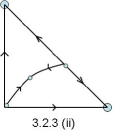
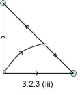
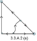
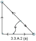

Figure 1: 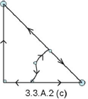
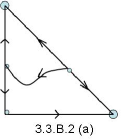
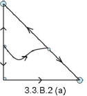

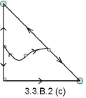
Figure 2: (b) The separatrix may behave in different ways. See Fig. 3.


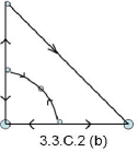
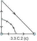
Figure 3: 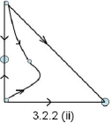
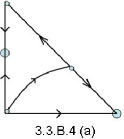
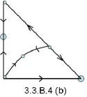
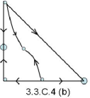
Figure 4: 
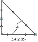
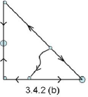
Figure 5: (d) The separatrix may behave in different ways. See Fig. 6.
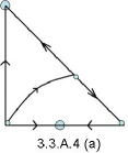
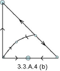
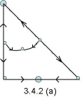
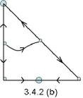

Figure 6: (e) The separatrix may behave in different ways. See Fig. 7.
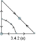
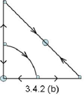
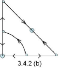
Figure 7: (f) The separatrix may behave in different ways. See Fig. 8.
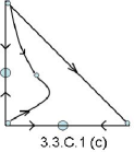
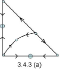
Figure 8: (g) The separatrix may behave in different ways. See Fig. 9.
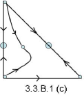

Figure 9: (h) The separatrix may behave in different ways. See Fig. 10.
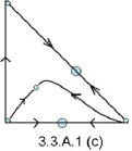
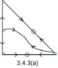
Figure 10: -
3.
There is only one pattern with three stable equilibria which must be the three vertices. (See Table 3.) The separatrix may behave in different ways. See Fig. 11.

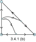
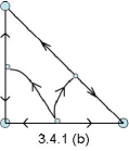
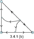
Figure 11:
5.2 Complete Dominance Case
In this subsection, we consider the case of complete dominance on at least one side of . There are altogether cases to consider and the number of patterns is greatly reduced in each case.
(i) Complete dominance on one side.
There are ways to assume complete dominance on one side.
(a) Suppose is completely dominant ( or ). The dynamics of (5.1) on is the same as being in the intermediate case. The dynamics on the other two edges will not be affected if is changed from intermediate case to complete dominance case. Therefore, to find all the patterns, we go through every case of being in the intermediate case in Tables 1-3 and examine how the signs of will change when the condition is replaced with or . There are such cases which generate patterns:
In the above means interior equilibrium. We observe that if , the pattern (Lemma 3.3.C.1(c) in Table 2) did not show up in our simulations. We now prove that this pattern cannot occur. From Table 2, sixth line from the bottom, we see that are in the superior case (). This and the fact imply that the signs of the Greek alphabets defined in (5.2) are
The signs of the eigenvalues of at are and . If are both stable, we have and . From (5.3), and which imply that cannot both be negative. Therefore, the pattern cannot occur. If , then among the above patterns, only the pattern (Lemma 3.3.C.1(b) in Table 1) cannot occur. The proof of this fact is similar and will be omitted.
(b) Suppose is completely dominant ( or . We repeat the process above and find that there are cases of being in the intermediate case which generate patterns:
However, if , the pattern (Lemma 3.3.B.1(c) in table 2) cannot occur. If , the pattern (Lemma 3.3.B.1(b) in table 1) cannot occur. The proof of these fact will be omitted.
(c) Suppose is completely dominant ( or . We repeat the process above and find that there are cases of being in the intermediate case which generate patterns:
However, if , the pattern (Lemma 3.3.A.1(c) in table 2) cannot occur and if , the pattern (Lemma 3.3.A.1(b) in table 1) cannot occur. The proof of these facts will also be omitted.
(ii) Complete dominance on two sides.
There are ways to assume complete dominance on two sides. The complete list is given below. They are all confirmed by computer simulations.
(a) and are completely dominant: .
(b) and are completely dominant: .
(c) and are completely dominant: .
(iii) Complete dominance on all sides.
There are ways to assume complete dominance on all sides. They all generate the same pattern .
6 Higher Number of Alleles
For alleles, , there are too many possible patterns that we cannot prove their existence like we did for the three-allele model in Section 5.1. We therefore resort to computer simulations to verify that certain patterns exist. We also develop some rules to show that certain patterns do not exist. For example, according to Proposition 4.5, we have
Rule 1. For any , if the interior equilibrium is stable, then no other equilibrium can be stable.
We say that three edge equilibria are coplanar if the edges they lie on form a triangle. From the results of the three-allele model, we have the following
Rule 2. The maximum number of coexisting stable equilibria in is and they must be the
three vertices. Hence, stable coplanar edge equilibria is not possible.
Rule 3. If the existing stable equilibria are all vertices, then they must include the vertex .
Rule 3 is a consequence of condition (1.2). We conjecture that it is valid for any .
6.1 Four-allele Model
The invariant set defined by (2.3) is a tetrahedron. It contains possible equilibria including vertices, edge equilibria, face equilibria, and one interior equilibrium. From the results of the three allele case, it is easy to see that the maximum number of coexisting stable equilibria is which we state below as rule 4. We first construct a table of all possible patterns and eliminate those that cannot exist using rules 1, 2 and 6 below. For example, the pattern (three stable vertices and one stable face equilibrium) is not possible because such a pattern would imply a three-allele model with two stable vertices and a stable edge equilibrium which violates rule 2. We also eliminate the patterns , and which are shown to be not possible in [16]. The remaining patterns are shown to exist by computer simulations and are summarized in Table 4 below. In the table, denotes the number of coexisting stable equilibria and denotes the number of patterns for the type indicated. If we add up all the numbers in the column, we see that the four-allele model has patterns. The last column in the table explains how the numbers in the column are obtained. For example, according to Table 4, there are patterns with one vertex equilibrium and one edge equilibrium; that is, . There are six edges in a tetrahedron and we can pair anyone (hence choices) with any one of the four vertices that does not lie in the edge. Since a tetrahedron has four vertices and each edge connects two vertices, the number of choices here is . The notation means choose which equals . Therefore, there are such patterns. We develop the following rules which will be used in the study of the five-allele model. The proof of rule 6 is rather involved and will not be presented here. Rule 5 follows from looking at Table 4.
Rule 4. The maximum number of coexisting stable equilibria in is .
Rule 5. If contains three or more stable equilibria, then none can be on a face except we can have a face with a stable equilibrium and two stable edge equilibria not on the face.
Rule 6. If the stable equilibria are all vertices, then they must include the vertex .
| pattern type | Explanations | |||||
| 1 | 1 | 1 | must be . | |||
| 1 | 6 | any one of the six edges. | ||||
| 1 | 4 | any one of the four faces. | ||||
| 1 | 1 | the interior equilibrium. | ||||
| 2 | 2 | 3 | any two vertices one of which must be . | |||
| 2 | 15 | any two edges: . | ||||
| 2 | 6 | any two faces: . | ||||
| 1 | 1 | 12 | pair any edge with a vertex not in the edge: . | |||
| 1 | 1 | 4 | pair any face with the one vertex not in the face. | |||
| 1 | 1 | 12 | pair any face with an edge not in the face: . | |||
| 3 | 3 | 3 | three vertices one of which must be : . | |||
| 3 | 16 | any three edges not coplanar: . | ||||
| 2 | 1 | 6 | pair any edge with the two vertices not in the edge. | |||
| 1 | 2 | 12 | pair any vertex with two edges not containing the vertex: | |||
| . Note two ends of an edge are vertices. | ||||||
| 2 | 1 | 12 | any face with two of the three edges not from the face. | |||
| 4 | 4 | 1 | all four vertices. | |||
| 4 | 3 | any four edges without forming a triangle: . | ||||
6.2 Five-allele Model
The set contains equilibria including vertices, edge equilibria, face equilibria, tetrahedral equilibria and interior equilibrium denoted by . There are at least patterns shown in the tables below. There are a few patterns which we cannot show nonexistence nor found them in our simulations. They are discussed at the end of this subsection.
| pattern type | Explanations | ||||||
| 1 | 1 | 1 | must be | ||||
| 1 | 10 | any one of the ten edges. | |||||
| 1 | 10 | any one of the ten faces. | |||||
| 1 | 5 | any one of the five tetrahedrons. | |||||
| 1 | 1 | the interior equilibrium. | |||||
| 2 | 2 | 4 | one of the two vertices must be . | ||||
| 2 | 45 | any two edges: | |||||
| 2 | 45 | any two faces: | |||||
| 2 | 10 | any two tetrahedrons: | |||||
| 1 | 1 | 30 | any edge and a vertex not in the edge: . | ||||
| 1 | 1 | 20 | any face and a vertex not in the face: . | ||||
| 1 | 1 | 5 | tetrahedron and the vertex not in the tetrahedron. | ||||
| 1 | 1 | 70 | any face with an edge not in the face: | ||||
| 1 | 1 | 20 | any tetrahedron and an edge not in the tetrahedron: | ||||
| . | |||||||
| 1 | 1 | 30 | any tetrahedron and a face not in the tetrahedron: | ||||
| . | |||||||
| 3 | 3 | 6 | one of the three vertices must be : . | ||||
| 3 | 110 | any three edges not coplanar: . | |||||
| 3 | 100 | any three faces not in a common tetrahedron: | |||||
| . | |||||||
| 2 | 1 | 30 | pair any edge with two vertices not in the edge: | ||||
| . | |||||||
| 2 | 1 | 10 | pair any face with the two vertices not in the face. | ||||
| 1 | 2 | 75 | any vertex with two edges not containing the vertex: | ||||
| . | |||||||
| 2 | 1 | 210 | pair any face with two edges not in the face: | ||||
| . | |||||||
| 2 | 1 | 30 | pair any tetrahedron with any two edges not in the | ||||
| tetrahedron: . | |||||||
| 2 | 1 | 75 | pair any tetrahedron with any two faces not in the | ||||
| tetrahedron: . | |||||||
| 1 | 2 | 180 | any edge with two faces not containing the edge and | ||||
| not in a common tetrahedron with the edge (an edge | |||||||
| is shared by three faces and three tetrahedrons): | |||||||
| . | |||||||
| pattern type | Explanations | ||||||
| 3 | 1 | 2 | 30 | pair any vertex with two faces not containing the vertex | |||
| (a vertex is shared by six faces): . | |||||||
| 1 | 1 | 1 | 60 | a face with a vertex not in the face and an edge neither | |||
| in the face nor containing the vertex: . | |||||||
| 1 | 1 | 1 | 60 | any tetrahedron with a face not in the tetrahedron plus | |||
| an edge neither in the tetrahedron nor in the face: | |||||||
| . | |||||||
| 4 | 4 | 4 | one of the four vertices must be : . | ||||
| 4 | 140 | any four edges without forming a triangle: | |||||
| . | |||||||
| 4 | 75 | see A below. | |||||
| 2 | 2 | 30 | pair any two vertices with any two edges not containing | ||||
| these vertices: . | |||||||
| 2 | 2 | 150 | see B below. | ||||
| 3 | 1 | 10 | pair any edge with the three vertices not in the edge. | ||||
| 1 | 3 | 80 | any three edges without forming a triangle from a | ||||
| tetrahedron (see pattern 3e in the four-allele model) | |||||||
| and the vertex not in the tetrahedron: . | |||||||
| 3 | 1 | 60 | see C below. | ||||
| 3 | 1 | 20 | pair any tetrahedron with any three edges not in the | ||||
| tetrahedron: . | |||||||
| 1 | 3 | 120 | see D below. | ||||
| 3 | 1 | 60 | see E below. | ||||
| 1 | 2 | 1 | 60 | pick two edges and one face from a tetrahedron and | |||
| choose the vertex not in the tetrahedron: . | |||||||
| (see pattern in four-allele model). | |||||||
| 5 | 5 | 1 | all five vertices. | ||||
| 5 | 72 | see F below. | |||||
| 5 | 12 | see G below. | |||||
| 1 | 4 | 15 | any four edges without forming a triangle from a | ||||
| tetrahedron (see pattern 4e in the four-allele model) | |||||||
| and the vertex not in the tetrahedron: . | |||||||
| 4 | 1 | 90 | type face with edges : . | ||||
| type face with edges : . | |||||||
| 3 | 2 | 60 | see H below. | ||||
| 6 | 6 | 10 | choose the six edges in any two tetrahedrons not on | ||||
| the common face of the two tetrahedrons: . | |||||||
To understand the explanation column of the above table, take the first pattern in Table 6. There are vertices and suppose a vertex, say vertex , is chosen. Then among the faces of , of them contains vertex . Therefore, faces do not contain vertex and there are ways to choose two of them. This explains why . The explanations of some the patterns in Table 6 are too complicated to fit into the space provided in the table and are explained below.
A. For the pattern, we observe that each face is shared by two tetrahedrons so there are actually faces if we take the tetrahedrons into account. According to Rule 5, each tetrahedron can contain at most 2 stable face equilibria. The faces may be put into the tetrahedrons in two ways: or . Consider the first way. There are patterns. The number may be explained as follows. Suppose we label the vertices through and we eliminate the tetrahedron . Consider one of the remaining four tetrahedrons, say . There are ways to choose faces from because the face , being on , is not eligible. But once we choose two of the faces, the other two faces on each of the remaining tetrahedrons are fixed. This explains the in the formula. For the second way, there are patterns so altogether we have patterns.
B. For the pattern, it is easy to see that the two faces chosen must have one common edge ( ways) or one common vertex ( ways because of symmetry). In each case, there are 6 ways to choose the two stable edge equilibria in order not to violate Rule 5. Thus, patterns are expected. However, the pattern with faces , and edges , is not show up in our simulations and we could not find it in any literature. There are such patterns. Therefore, there are at least and at most patterns.
C. For the pattern, first pick one of the faces, then choose edges such that they are not coplanar (Rule 2), none of them is from the face chosen (Rule 1), and they and the face are not in a common tetrahedron (Rule 5). Accordingly, there are patterns expected. But only patterns of the type face with edges , , ( patterns) show up in our simulations, whereas the patterns of the type face with edges , , ( patterns), of the type face with edges , , ( patterns), and of the type face with edges , , ( patterns) do not show up in our simulations. Therefore, there are at least and at most 3e+1f patterns.
D. For the pattern, there are two types of patterns. For type 1, first pick one of the faces, say, as face , then face 2 is determined by vertex and any edge of face , say, , face is determined by vertex and any edge of face but not used by face , say, . The stable edge equilibrium is on . There are patterns of type 1. For type 2, first pick two of the faces with a common edge ( ways), say, and , then the third face is decided by the left vertex and the two vertices not on the common edge of the first two faces. Lastly, the stable edge equilibrium could be either on or . There are patterns of type 2.
E. For the pattern, first pick any tetrahedron, say, . To decide the three faces, we pick three edges from which are not coplanar and not all from the same vertex, say, , , , then the three faces are determined by vertex and these three edges respectively, namely, , , . There are total patterns.
F. For the pattern, we observe that there are ways to choose edges from the edges but we must subtract cases of one coplanar edges and cases of two coplanar edges which will result in only 5e patterns. To see that there are one coplanar edges, suppose the coplanar edges are the sides of the triangle (we have such triangles). Then the remaining two edges can be chosen two ways (so that we don’t have two coplanar edges). One way is to choose the edge and then the fifth edge may be chosen from any of the six edges ,. A second way is to choose one edge from the group and another edge from the group with a total of choices. Hence, there are ways to choose the other two edges besides the sides of the triangle . Therefore, there are cases of one coplanar edges. The argument for the two coplanar edges is similar and will be omitted.
G. For the pattern, each face is shared by two tetrahedrons so there are actually faces if we take the tetrahedrons into account and each tetrahedron has exactly two stable face equilibria. Choose two faces (6 ways) from the first tetrahedron , say, and . Then in the second tetrahedron , we choose one more face either or . The two faces chosen in the rest tetrahedrons are fixed now. Thus, there are ways.
H. For the pattern, choose any two faces with a common edge (30 ways), say, and , then choose three edges out of such that they are not in a common tetrahedron with either or by Rule 5. Thus, there are ways.
We cannot find the following patterns in our simulations nor can we prove their nonexistence: , , , , some types of (see B above), and some types of (see C above). From the tables we observe the following rules which may be used to study the six-allele model:
Rule 7. The maximum number of coexisting stable equilibria for the five-allele model is with
all stable equilibria on the edges.
Rule 8. If there are five stable equilibria, none of them can be in the interior of a tetrahedron.
Rule 10. If the stable equilibria are all vertices in five-allele case, then one of them must be
.
6.3 Computer Simulations
In this section we briefly describe how one can perform computer simulations to help find patterns for higher number of alleles. One possible idea which we adopted is the following. First write a computer program that randomly generates a fitness matrix that satisfies condition (1.2). Then use the method described in Remark 4.3 to compute and count the number of negative eigenvalues at each existing equilibrium. Note that for alleles, there are a maximum possible equilibria. Write the results of the computer program to a text file. Each line in the text file should contain integers representing the number of negative eigenvalues of the Jacobian matrix evaluated at that particular equilibrium. A special symbol should be used in case the equilibrium does not exist. Run a sorting algorithm on the text file that will turn each line into a pattern (see example below). One needs to repeat this process several times, each time with increasing number of simulations until no new patterns are found.
As an example, suppose we want to find all the patterns for the three-allele model. Then a line in our output text file may look like , which means that the three vertices have and negative eigenvalues, respectively, have and negative eigenvalues, respectively, and and the interior equilibrium do not exist for this round of simulation ( means the corresponding equilibrium does not exist). Of course another fitness matrix will generate a different line of numbers. The sorting algorithm will turn this line into the pattern and write it to a file called ”filename.2” which contains all distinct patterns with two stable equilibria. “filename” is a user supplied name and the sorting algorithm also removes duplicate patterns. At the end, the sorting algorithm produces three files: ”filename.1”, ”filename.2” and ”filename.3”. ”filename.1” contains distinct patterns with one stable equilibrium (see Table 1), ”filename.2” contains distinct patterns with two stable equilibria (see Table 2) and ”filename.3” contains distinct patterns with three stable equilibria (see Table 3).
Some patterns are difficult to find if is large. For example, for the five-allele case, we need to simulate over million times until no new patterns are found and yet we are not sure if we found them all. For the six-allele case, we used processors and simulated over million times and found over distinct patterns. Of course, not finding a pattern does not mean that pattern does not exist unless its absence can be proved theoretically. We believe that the number of patterns increases exponentially with .
7 Conclusion
In this paper, we list all patterns for the three- and four-allele selection models and almost all patterns for the five-allele selection model for all fitness matrices satisfying condition (1.2). A pattern is simply the number and locations in the invariant set of all coexisting stable equilibria. In our investigation, we do not assume the truth of the conjecture of Cannings and Vickers that any subset of a pattern is also a pattern [16, 5]. Knowing the patterns is important because it tells us the possible long-term genetic makeup of the population; that is, which alleles will survive and which will disappear under selection forces in the long run. For the three-allele model, we prove our results analytically and show the separatrices for each pattern so that we know the asymptotic behavior of the solutions of the mathematical model (1.1) as . We also consider the case of complete dominance for the three-allele model. Through the use of computer simulations and the rules we developed, we show that there are patterns for the four-allele model and at least patterns for the five-allele model. There are a few patterns in the five-allele model that did not show up in our computer simulations but we are not able to show that they do not exist. For the six-allele model, parallel computer simulations indicate that there are over patterns. We conjecture that the number of patterns grow exponentially as the number of alleles increases. In this paper, we also prove several interesting mathematical results in Section 4 some of which we believe are new.
8 Acknowledgments
We thank Allan E. Johannesen of the WPI Computing and Communications Center for writing the sorting algorithm to help us recognize patterns. We also thank Siamak Najafi and Adriana Hera for their help with parallel computing for the six-allele case. Finally, we thank Jesse Bowers for helpful discussions on Lemmas 5.1 - 5.4.
References
- [1] an der Heiden, U., On manifolds of equilibria in the selection model for multiple alleles, J. Math. Biol. 1 (1975) 321-330.
- [2] Broom, M., C. Cannings and G. T. Vickers, On the number of local maxima of constrained quadratic form, Proc. R. Soc. Lond. A 443 (1993) 573-584.
- [3] Bürger, R., The mathematical theory of selection, recombination, and mutation, Wiley, 2000.
- [4] C. Cannings and G. T. Vickers, Patterns of ESS’s II, J. Theo. Bio. 132 (1988) 409-420.
- [5] C. Cannings and G. T. Vickers, Patterns and invasions of evolutionarily stable strategies, J. Appl. Maths and Computation 32 (1989) 227-253.
- [6] C. Cannings and G. T. Vickers, The genealogy of patterns of ESS’s, Selected Proceedings of the Sheffield Symposium on Applied Probability, IMS Lecture Notes Monogr. Ser. 18 (1991) 193-204.
- [7] L. Edelstein-Keshet, Mathematical Models in Biology, Society for Industrial and Applied Mathematics, Philadelphia,1988.
- [8] P.J. Hughes and E. Seneta, Selection equilibria in a multi-allele single-locus setting, Heredity 35 (1975) 185-194.
- [9] J.F. C. Kingman, A mathematical problem in population genetics, Proc. Camb. Phil. Soc. 57 (1961) 574-582.
- [10] J.F.C. Kingman, On an inequality in partial averages, Quart. J. Math. 12 (1961) 78-80.
- [11] S.P.H. Mandel, The stability of a multiple allellic system, Heredity 13 (1959) 289-302.
- [12] S.P.H. Mandel, The equivalence of different sets of stability conditions for multiple allelic systems, Biometrics 26 (1970) 840-845.
- [13] T. Nagylaki, Introduction to Theoretical Population Genetics, Springer, N.Y. 1992.
- [14] P.J. Hughes and E. Seneta, Selection equilibria in a multi-allele single-locus setting, Heredity 35 (1975) 185-194.
- [15] G. Strang, Linear algebra and its applications, Third Edition, Thomas Learning, 1998.
- [16] G.T. Vickers and C. Cannings, Patterns of ESS’s I, J. Theo. Bio. 132 (1988) 387-408.