Hydrogen cyanide and isocyanide in prestellar cores

Abstract

Aims. We studied the abundance of HCN, H¹³CN, and HN¹³C in a sample of prestellar cores, in order to search for species associated with high density gas.

Methods. We used the IRAM 30m radiotelescope to observe along the major and the minor axes of L1498, L1521E, and TMC 2, three cores chosen on the basis of their CO depletion properties. We mapped the $J=1\rightarrow 0$ transition of HCN, H¹³CN, and HN¹³C towards the source sample plus the $J=1\rightarrow 0$ transition of N₂H⁺ and the $J=2\rightarrow 1$ transition of C¹⁸O in TMC 2. We used two different radiative transfer codes, making use of recent collisional rate calculations, in order to determine more accurately the excitation temperature, leading to a more exact evaluation of the column densities and abundances.

Results. We find that the optical depths of both H¹³CN(1$-$0) and HN¹³C(1$-$0) are non-negligible, allowing us to estimate excitation temperatures for these transitions in many positions in the three sources. The observed excitation temperatures are consistent with recent computations of the collisional rates for these species and they correlate with hydrogen column density inferred from dust emission. We conclude that HCN and HNC are relatively abundant in the high density zone, $n({\rm H}_{2})\sim 10^{5}$ cm^-3, where CO is depleted. The relative abundance [HNC]/[HCN] differs from unity by at most 30% consistent with chemical expectations. The three hyperfine satellites of HCN(1$-$0) are optically thick in the regions mapped, but the profiles become increasingly skewed to the blue (L1498 and TMC 2) or red (L1521E) with increasing optical depth suggesting absorption by foreground layers.

1 Introduction

Tracing the dense central regions of prestellar cores is essential for an understanding of their kinematics and density distribution. Many of the well studied nearby cores are thought to be static with a ”Bonnor-Ebert” radial density distribution (see Bergin & Tafalla bt07 (2007) and references therein) comprising a roughly $1/r^{2}$ fall off surrounding a central region of nearly constant density. However, our understanding of the central regions with H₂ number densities of $10^{5}$ cm^-3 or more is limited both by our uncertainties about dust emissivity and molecular abundances. Dust emission, because it is optically thin, is a useful tracer of mass distribution, but both temperature gradients and gradients in the dust characteristics (refractive index and size distribution) mean that dust emission maps should be interpreted with caution. Molecular lines offer the advantage that they permit an understanding of the kinematics, but depletion and other chemical effects render them often untrustworthy. Depletion is more rapid at high density and low temperature and these are just the effects that become important in the central regions of cores.

One interesting result from studies to date (e.g. Tafalla et al. tm06 (2006)) is that the only molecular species to have a spatial distribution similar to that of the optically thin dust emission are N₂H⁺ and NH₃, consisting solely of nitrogen and hydrogen. This is in general attributed to the claim that their abundance is closely linked to that of molecular nitrogen (one of the main gas phase repositories of nitrogen) which is highly volatile and hence one of the last species to condense out (Bisschop et al. bf06 (2006)). However N₂ is only marginally more volatile than CO which is found observationally to condense out at densities of a few 10⁴ cm^-3 (Tafalla et al. tm02 (2002), 2004a ) and it has thus been puzzling to have a scenario where C-containing species were completely frozen out but N₂ not. This has led to a number of models aimed at retaining gas phase nitrogen for at least a short time after CO has disappeared, e.g. Flower et al. fp06 (2006), Akyilmaz et al. af07 (2007), and Hily-Blant et al. hw10 (2010) (hereafter paper I). There have also been attempts to obtain convincing evidence for the existence in the gas phase of species containing both C and N at densities above a few 10⁵ to 10⁶ cm^-3 at which CO depletes (e.g. Hily-Blant et al. hw08 (2008) and paper I). A partial success in this regard was obtained by Hily-Blant et al. hw08 (2008) who found that the intensity of ¹³CN(1$-$0) behaved in similar fashion to the dust emission in two of the densest cores: L183 and L1544. The implication of this is that at least some form of carbon, probably in the form of CO, remains in the gas phase in these objects at densities above $10^{5}$ cm^-3. Thus, a tentative conclusion is that the CO abundance at densities above 10⁵ cm^-3 is much lower than the canonical value of $10^{-4}$ relative to H₂ (Pontoppidan p06 (2006)), but nevertheless sufficiently high to supply carbon for minor species.

Putting this interpretation on a more solid foundation requires observation of possible tracers of the depleted region in cores carried out in a manner which will permit distinguishing species associated with high density gas from those present in the surrounding lower density envelope. This is complicated though perhaps facilitated by the gradients in molecular abundance due to depletion. While molecular abundances in general are expected to drop at high densities when depletion takes over, this is not necessarily true for all species at least within a limited density range (see the results for deuterated species discussed by Flower et al. fp06 (2006)). However, proving that one is observing emission from high density gas involves either showing that one can detect transitions which require high densities to excite or showing that the emission comes from a compact region coincident with the dust emission peak. The former is rendered more difficult by the temperature gradients believed to exist in some cores (see e.g. Crapsi et al. cc05 (2005)). The latter requires highly sensitive high angular resolution observations. A combination of the two is likely to be the best strategy.

One approach to these problems which has not been fully exploited to date is to make use of the hyperfine splitting present in essentially all low lying transitions of N-containing species. It is clear in the first place that the relative populations of hyperfine split levels of species such as HCN and CN are out of LTE in many situations (see Walmsley et al. wc82 (1982), Monteiro & Stutzki ms86 (1986), and paper I). Interpreting such anomalies requires accurate collisional rates between individual hyperfine split levels, but such rates can be determined from the rates between rotational levels (e.g. Monteiro and Stutzki ms86 (1986)) and clearly in principle, they allow limits to be placed on the density of the emitting region. It is also the case that species of relatively low abundance like H¹³CN are found to have rather minor deviations from LTE between hyperfine levels of the same rotational level (see paper I) and in this case, one can determine the line excitation temperature and optical depth based on the relative hyperfine satellite intensities. While this is clearly doubtful procedure in that the non-LTE anomalies can cause errors in the inferred optical depth, it is nevertheless (as we shall discuss) an approach which can give a zero order estimate of relative rotational level populations and hence of the local density.

In the case of more abundant species such as the main isotopologues of HCN or CN, one finds that ”self absorption” or absorption in foreground relatively low density material can obliterate any signal from the high density central regions of a core. However, from these tracers, one can in principle glean information on the kinematics of foreground layers of the core. Thus, one can hope to find evidence for infall. We indeed find in this study that profiles change in gradual fashion as a function of transition line strength and this does indeed yield evidence for either infall or expansion of foreground layers.

Here we extend the results of paper I to three other cores which have been chosen on the basis of their CO depletion properties (see e.g. Bacmann et al. bl02 (2002), Brady Ford & Shirley bs11 (2011)). We in particular chose objects with large CO depletion holes indicative of a relatively large age. This might occur for example in sources where magnetic field is capable of slowing down or preventing collapse. We also used as a guide the angular size measured in the N₂H⁺(1$-$0) transition by Caselli et al. (2002b ) which is thought to correspond roughly to the area of CO depletion. Thus, we chose the cores L1498 and TMC 2 which appear to have large CO depletion holes (0.08 parsec in the case of TMC 2). As a comparison source, we included in our study L1521E, which shows little or no depletion in C-bearing species (Tafalla & Santiago 2004b ).

In this paper then, we present IRAM 30m observations of the $J=1\rightarrow 0$ transition of HCN, H¹³CN and HN¹³C along the major and the minor axes of the three selected sources, L1498, L1521E and TMC 2, as well as the $J=1\rightarrow 0$ transition of $\mathrm{N_{2}H^{+}}$ and the $J=2\rightarrow 1$ transition of C¹⁸O towards TMC 2. In Sect. 2, we discuss the observational and data reduction procedures, summarising the results in Sect. 3. In Sect. 4 we compare the distribution of the line emission with respect to the dust emission, investigating about the presence of depletion. In Sect. 5 we describe the evidence of the asymmetry of the HCN(1$-$0) line profiles. In Sect. 6 we explain the methods used for determining the excitation temperature, while in Sect. 7 we give the estimated column densities and abundances for the observed lines. In Sect. 8 we give our conclusions. Comment on non-LTE hyperfine populations are provided in Appendix A, while in Appendix B we summarise the spectroscopic data and observational parameters of the observed molecules.

2 Observations

L1498, L1521E, and TMC 2 were observed in July 2008, using frequency switching and raster mode, with a spacing of 20^′′, 25^′′ and 50^′′, respectively, along the major and the minor axes. The axes were identified from the continuum emission maps showed in Tafalla et al. (tm02 (2002)) for L1498, Tafalla et al. (2004a ) for L1521E, and Crapsi et al. (cc05 (2005)) for TMC 2. Observing parameters are given in Table 4.

Observations of the 89 GHz HCN(1$-$0) and the 86 GHz H¹³CN(1$-$0) multiplets (see Table 2) plus the 87 GHz HN¹³C(1$-$0) multiplet (see Table 3) were carried out using the VESPA autocorrelator with 20 kHz channel spacing (corresponding to about 0.069 km s^-1) with 40 MHz bandwidth for HCN(1$-$0) and 20 MHz bandwidth for H¹³CN(1$-$0) and HN¹³C(1$-$0). The final rms, in $T_{\rm mb}$ unit is $\sigma_{\rm T}\sim 50$ mK, $\sim 20$ mK, and $\sim 30$ mK for HCN(1$-$0), H¹³CN(1$-$0), and HN¹³C(1$-$0), respectively.

Observations of the 93 GHz N₂H⁺(1$-$0) multiplet and of the 219 GHz C¹⁸O(2$-$1) line were carried out in TMC 2 using 10 kHz channel spacing with 40 MHz bandwidth for $\mathrm{N_{2}H^{+}}$(1$-$0) and 20 kHz channel spacing with 40 MHz bandwidth for C¹⁸O(2$-$1). For $\mathrm{N_{2}H^{+}}$  the final rms, in $T_{\rm mb}$ units, in channels of width $\delta v=0.031$ km s^-1, is $\sigma_{\rm T}\sim 100$ mK while for C¹⁸O(2$-$1), the final rms (channels of width $\delta v=0.027$ km s^-1) is $\sigma_{\rm T}\sim 250$ mK.

Data reduction and analysis were completed using the CLASS software of the GILDAS facility, developed at the IRAM and the Observatoire de Grenoble. In what follows, all temperatures are on the main-beam scale, $T_{\rm mb}=F_{\rm eff}T_{\rm A}^{*}/B_{\rm eff}$, where $T_{\rm A}^{*}$ is the antenna temperature corrected for atmospheric absorption, while B_eff and F_eff are the beam and the forward efficiencies, respectively (see Table 4 for the numerical values of efficiencies).

3 Observational results

Figure 1 shows the continuum emission of the three cores together with the positions mapped in lines described in Sect. 2. The selected sources have already been widely observed in the past as possible tracers of conditions in the high density core nucleus. We succeeded in observing HN¹³C(1$-$0) and the three hyperfine components of HCN(1$-$0) and H¹³CN(1$-$0).

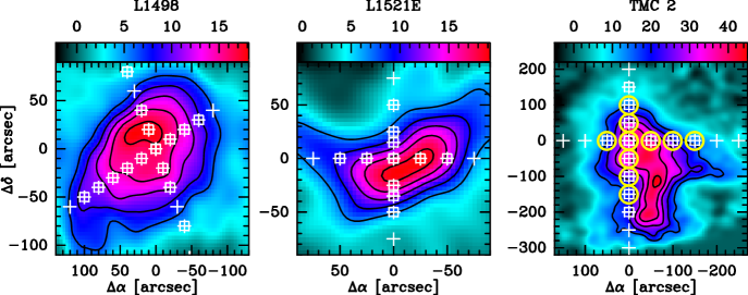
Figure 1: Observed positions in L1498 (left panel), L1521E (middle panel), and TMC 2 (right panel), superposed on the dust emission map smoothed to 28^′′, from Tafalla et al. (tm02 (2002)), Tafalla et al. (2004a ), and Crapsi et al. (cc05 (2005)), respectively. Mapped positions in HCN(1$-$0) (white crosses), H¹³CN(1$-$0) and HN¹³C(1$-$0) (white squares), and N₂H⁺(1$-$0) (yellow circles). Contours represent 35, 50, 65, 80 and 95 per cent of the peak value of the dust emission which is 18.0, 21.0, and 45.0 mJy/(11^′′ beam) for L1498, L1521E, and TMC 2, respectively. The (0,0) position corresponds to $\alpha(2000)=04^{\rm h}10^{\rm m}51.5^{\rm s}$, $\delta(2000)=25^{\circ}09^{\prime}58^{\prime\prime}$ for L1498, to $\alpha(2000)=04^{\rm h}29^{\rm m}15.7^{\rm s}$, $\delta(2000)=26^{\circ}14^{\prime}05^{\prime\prime}$ for L1521E, and to $\alpha(2000)=04^{\rm h}32^{\rm m}48.7^{\rm s}$, $\delta(2000)=24^{\circ}25^{\prime}12^{\prime\prime}$ for TMC 2.

Figure 2 shows a comparison of the line profiles for the different tracers. We plotted the weakest ($F=0\rightarrow 1$) component of HCN(1$-$0) at 88633.936 MHz, the strongest ($F=2\rightarrow 1$) component of H¹³CN(1$-$0) at 86340.184 MHz, HN¹³C(1$-$0) at 87090.675 MHz, the isolated component ($F_{1},F=0,1\rightarrow 1,2$) of $\mathrm{N_{2}H^{+}}$(1$-$0) at 93176.2650 MHz, and the C¹⁸O(2$-$1) transition at 219560.319 MHz. We used the components enumerated here also for the comparison between line and dust emission described below, supposing them to be the most optically thin. The offsets for each source are relative to the dust peak emission (see caption of Fig. 1).

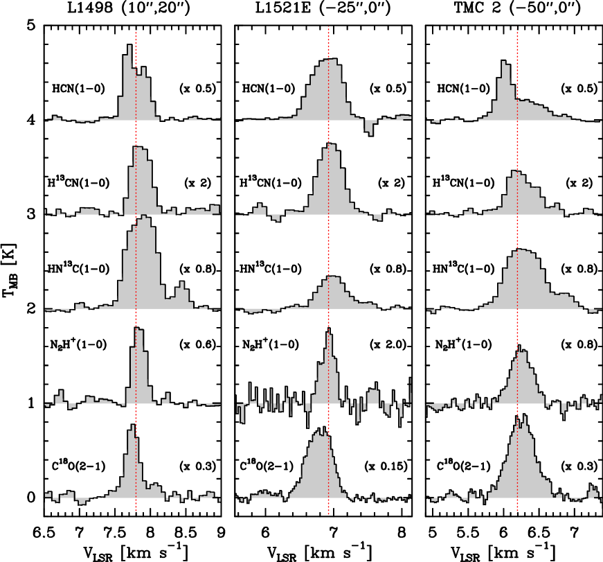
Figure 2: Emission line for the different tracers of the source sample towards the dust emission peak. The 88633 MHz component of HCN(1$-$0) is shown together with the 86340 MHz component of H¹³CN(1$-$0), HN¹³C(1$-$0), the 93176 MHz isolated component of $\mathrm{N_{2}H^{+}}$(1$-$0), and C¹⁸O(2$-$1). Spectra have been multiplied by a scaling factor to allow the simultaneous comparison. Red dotted lines show the systemic LSR velocity of the sources evaluated from the well-determined frequencies of $\mathrm{N_{2}H^{+}}$(1$-$0), see Pagani et al. (pd09 (2009)).

There are clear trends in the line widths which we derive for our three sources with values of order 0.2 km s^-1 for L1498, 0.3 km s^-1 for L1521E, and 0.45 km s^-1 for TMC 2. Besides, we noticed that there is a reasonable agreement between the systemic velocity, $V_{\rm LSR}$, of $\mathrm{N_{2}H^{+}}$ and H¹³CN to within 0.08 km s^-1, while line widths of H¹³CN seem larger by 0.05 km s^-1 with respect to $\mathrm{N_{2}H^{+}}$, but this may be due to ¹³C hyperfine splitting (Schmid-Burgk et al. sm04 (2004)).

There is a clear difference between the HCN and H¹³CN profiles in the three sources: while in L1521E, the HCN profile is broader than its isotopologue, in L1498 and TMC 2, HCN and H¹³CN have very different profiles, presumably because of high optical depth in HCN.

All these molecules show hyperfine structure, although in the case of HN¹³C it is not possible to avoid the blending of the components, and the hyperfine fitting has been conducted using the HFS method in CLASS. To fit this line, we followed van der Tak et al. (vdtm09 (2009)) who found that it consists of eleven hyperfine components which can however be reduced to four “effective” components. As an instance, in the upper panel of Fig. 3, we show the fit of the HN¹³C line at the offset $(10,20)$ towards L1498 together with the four distinguishable hyperfine components. The fit gives a value for the total optical depth equal to $\tau=4.58\pm 0.32$ and all the observed points show similar values, as shown in Figure 4, with an average of $\langle\tau\rangle=5.16\pm 0.86$. Also for H¹³CN we found a good simultaneous fit of the three hyperfine components (see lower panel of Fig. 3) and, as HN¹³C, this line is somewhat optically thick with a total optical depth of $\tau=3.11\pm 0.77$ at the offset $(10,20)$ and a mean optical depth of $\langle\tau\rangle=4.34\pm 1.15$. Hence one can expect the optical depth in HCN hyperfine components to be of order 30–100 assuming the canonical isotopic ratio for $[^{12}$C]/$[^{13}$C] of 68 (Milam et al. ms05 (2005)).

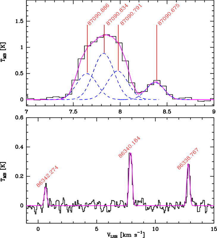
Figure 3: HN¹³C(1$-$0) (upper panel) and H¹³CN(1$-$0) (lower panel) emission towards L1498 at the offset $(10,20)$; black solid histogram, hyperfine components used for the fit, blue dashed lines, centred at the frequencies listed in Table 3, and line fit, magenta solid line.

Figure 4: Total optical depth of HN¹³C(1$-$0), solid squares, and H¹³CN(1$-$0), empty squares, for all the observed positions in L1498 as a function of the molecular hydrogen column density.

4 Probing the presence of depletion

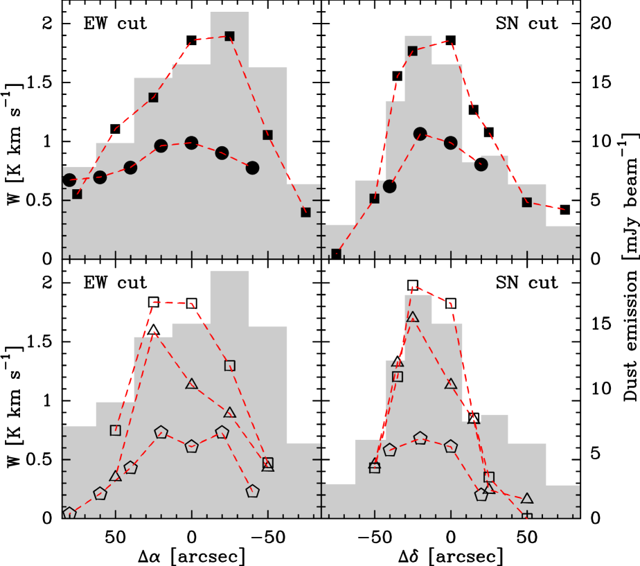
Figure 7: Comparison between the dust emission (gray histograms) and the integrated intensity of the observed species along the two cuts in L1521E. Upper panels: solid squares, HCN(1$-$0) [$\times 2.5$]; solid circles, C¹⁸O(2$-$1) [$\times 0.4$]. Lower panels: empty triangles, H¹³CN(1$-$0) [$\times 27$]; empty squares HN¹³C(1$-$0) [$\times 5.5$]; empty pentagons, N₂H⁺(1$-$0) [$\times 10$]. The typical error on the integrated intensity is about 20 mK km s^-1.

In this section, we study the dependence of the integrated intensity, $W$, of the HCN, H¹³CN and HN¹³C transitions on offset from the dust emission peaks. In the case of HCN, we consider the weakest $F=0\rightarrow 1$ line and in the case of H¹³CN, the strongest $F=2\rightarrow 1$ satellite. The observational results are shown in Figures 6, 7, and 8 where we compare the observed intensity of these lines with the dust emission which is taken to be representative of the H₂ column density. It is useful first to comment briefly on what one can expect qualitatively to learn from such studies.

One notes in the first place that optically thick transitions, due to scattering and line saturation, are naturally likely to have a broader spatial distribution than thin (or very moderate optical depth) transitions. Thus, the HCN($F=0\rightarrow 1$) transition can be expected to be roughly an order of magnitude more optically thick than H¹³CN($F=2\rightarrow 1$) assuming the local interstellar [¹²C]/[¹³C] ratio (Milam et al. ms05 (2005)) and no fractionation. One thus expects a broader spatial distribution of HCN than H¹³CN and indeed this is confirmed by the results shown in all the three sources. For example, the half power size of HCN in L1498 along the NW-SE cut is 170^′′ as compared with 120^′′ for H¹³CN and HN¹³C, and 180^′′ for the dust emission. One concludes that the ¹³C substituted isotopologue is a much better tracer of HCN column density than the more abundant form even when using the weakest hyperfine component.

However, one also notes from these figures that the C¹⁸O distribution is essentially flat as has been seen in a variety of studies (Tafalla et al. tm02 (2002), 2004a ). This has been attributed to depletion of CO at densities $n$(H₂) above a critical value of order a few times 10⁴ cm^-3 and our observations are entirely consistent with this. It is also true however (see also Tafalla et al. tm06 (2006) and paper I) that species like H¹³CN and HN¹³C, while they clearly have different spatial distributions from the dust emission, have half power sizes which are roughly similar (see results for L1498 above). Such effects clearly do not apply to $\mathrm{N_{2}H^{+}}$ which does not contain carbon and which in general has been found to have a spatial distribution similar to that of the dust (Tafalla et al. tm06 (2006)). However, one sees in Fig. 6 – 8 that HN¹³C and H¹³CN have a spatial distribution closer to that of the dust emission and we conclude that these two isotopologues may often be very useful tracers of kinematics as N₂H⁺ at densities above the critical values at which CO depletes. It is possible that CO, while depleted by roughly an order of magnitude relative to the canonical [CO]/[H${}_{2}]$ abundance ratio of 10^-4, is nevertheless sufficiently abundant to account for minor species such as HCN and HNC.

Finally, we note from Fig. 8 that towards TMC 2, where the dust peak H₂ column density is larger than in the other two sources, there seems to be a good general accord between the dust emission and the intensity of HN¹³C, H¹³CN, and $\mathrm{N_{2}H^{+}}$. The CO however has again a flat distribution suggesting once more that it is depleted in the vicinity of the dust peak. There is no reason in this source to suppose that $\mathrm{N_{2}H^{+}}$ traces the high density gas around the core nucleus better than the ¹³C substituted isotopologues of HCN and HNC. There are however slight differences close to the dust peak between the different species which are perhaps attributable to excitation and optical depth effects, but could also be caused by the depletion which presumably all molecules undergo if the density is sufficiently high. We conclude that cyanides and isocyanides are useful tracers of gas with densities around $10^{5}$ cm^-3.

We note that models of a collapsing prestellar core indeed suggest that HCN and HNC should remain with appreciable gas-phase abundance at an epoch when the CO abundance has depleted to a few percent of the canonical value of $10^{-4}$ relative to H₂. To illustrate the differential freeze out of HCN relative to that of CO found in the chemical models, Fig. 5 displays the depletion of HCN as a function of the depletion of CO computed in the collapsing gas, starting from steady-state abundances at a density of 10⁴ cm^-3. The numerical gravitational collapse model is described in Sect. 6.2 of Hily-Blant et al. (hw10 (2010)). Two models are shown for two different collapse time scale: free-fall time ($t_{\rm ff}$) and $10t_{\rm ff}$. It may be seen from Fig. 5 that the depletion of HCN relative to that of CO strongly depends on the collapse time scale: the model shows that HCN is depleted on longer timescales than CO, in particular if the dynamical timescale is several free fall times. HNC, not shown in the plot, has the same behaviour of HCN.

Figure 5: The HCN depletion as a function of the CO depletion during the collapse, computed by the gravitational collapse model of Hily-Blant et al. (hw10 (2010)), see their Fig. 8. Values are normalised with respect to the initial abundances. Each point is labelled with the time of the collapsing gas. Two models are shown: a free fall model labelled $t_{\rm ff}$ (red dashed curve) and a collapsing model with a time scale multiplied by a factor ten, labelled $10t_{\rm ff}$ (blue solid curve). The black dotted curve shows the positions of equal depletion for CO and HCN.

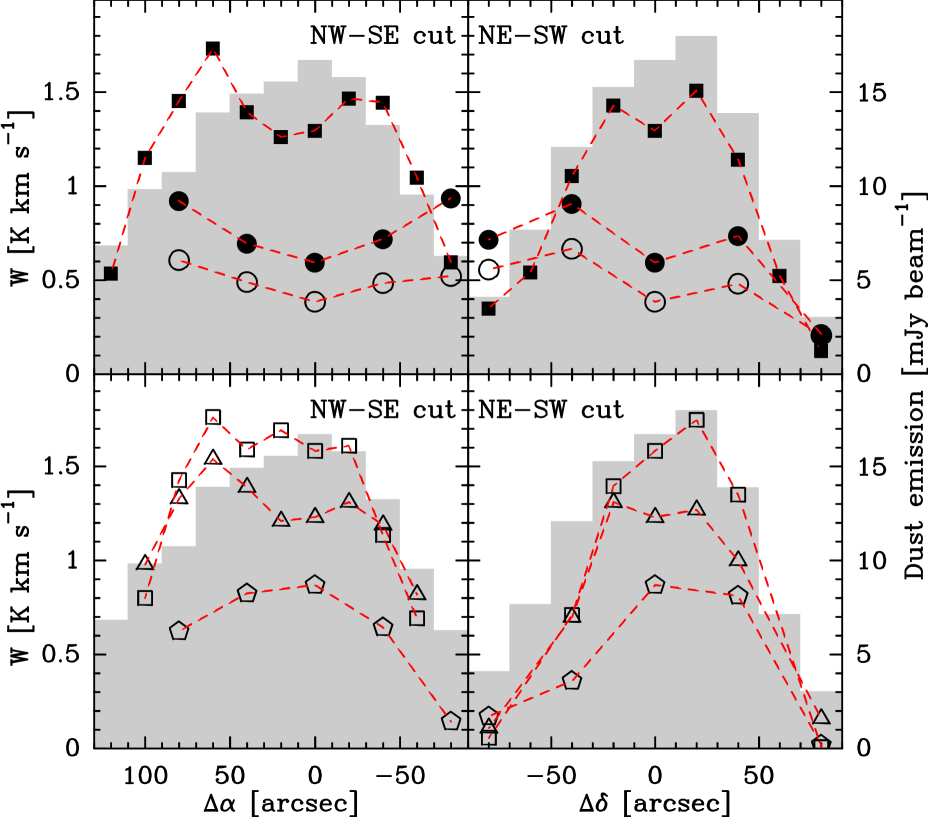
Figure 6: Comparison between the dust emission (gray histograms) and the integrated intensity of the observed species along the two cuts in L1498. Upper panels: solid squares, HCN(1$-$0) [$\times 3$]; empty circles, C¹⁸O(1$-$0) [$\times 0.8$]; solid circles, C¹⁸O(2$-$1) [$\times 1.4$]. Lower panels: empty triangles, H¹³CN(1$-$0) [$\times 10$]; empty squares, HN¹³C(1$-$0) [$\times 2.5$]; empty pentagons, N₂H⁺(1$-$0) [$\times 3$]. The typical error on the integrated intensity is about 20 mK km s^-1.

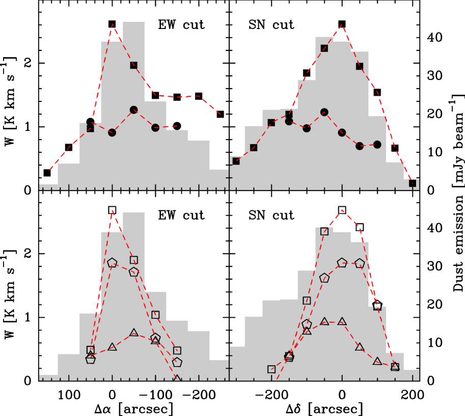
Figure 8: Comparison between the dust emission (gray histograms) and the integrated intensity of the observed species along the two cuts in TMC 2. Upper panels: solid squares, HCN(1$-$0) [$\times 4$]; solid circles, C¹⁸O(2$-$1). Lower panels: empty triangles, H¹³CN(1$-$0) [$\times 25$]; empty squares, HN¹³C(1$-$0) [$\times 3.5$]; empty pentagons, N₂H⁺(1$-$0) [$\times 4.5$]. The typical error on the integrated intensity is about 20 mK km s^-1.

5 Line profiles

In this Section, we discuss the behaviour of the HCN line profiles as a function of optical depth. It is clear from Fig. 2 that towards L1498 and TMC 2, the $F=0\rightarrow 1$ component of HCN has a profile skewed to the blue relative to $F=2\rightarrow 1$ of H¹³CN and it is tempting to interpret this as being due to absorption in a foreground infalling layer. Fig. 9 illustrates this well showing all three HCN components compared with the strongest $F=2\rightarrow 1$ component of H¹³CN. One sees that there is in fact a progression going from the highly skewed optically thick $F=2\rightarrow 1$ component of HCN to the essentially symmetric profile of H¹³CN. In the following, we attempt to quantify this trend.

Looking at Fig. 9, related to the three hyperfine components of HCN and the H¹³CN($F=2\rightarrow 1$) component, one can qualitatively argue that the greater the relative intensity of a line, the higher is the skewness degree. It can be seen that the H¹³CN($F=2\rightarrow 1$) component (gray histogram) is fairly symmetric and indeed, as seen earlier, its optical depth is not high since it is next to optically thin limit, but HCN components are skewed towards the blue in L1498 and TMC 2, while in L1521E they are skewed towards the red.

The superposition of the different hyperfine components of HCN led us to the discovery of a correlation between the line profile and its intensity. In particular, a red-absorbed line profile (that is skewed towards the blue) is a hint for the presence of an outer layer which is absorbing the emission of the inner layer while moving away from the observer, suggesting infall motions. Conversely, a blue-absorbed line profile (that is skewed towards the red) is an indication of the motion of the outer absorbing layer towards the observer, that is outflow motions.

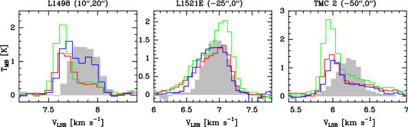
Figure 9: Superposition of the three hyperfine components of HCN(1$-$0) ($F=1\rightarrow 1$, red line; $F=2\rightarrow 1$, green line; $F=0\rightarrow 1$, blue line) with the strongest component ($F=2\rightarrow 1$, gray histograms) of H¹³CN(1$-$0) [$\times$4], see Table 2 for component indices. In order to compare line shapes and intensities, components have been shifted in frequency.

To quantify these deviations from the expected Gaussian shape in the optically thin limit, we compared the asymmetry degree towards the different positions mapped, using the definition of skewness, $\delta V$, given by Mardones et al. (mm97 (1997))

$$\delta V=\frac{V_{\rm thick}-V_{\rm thin}}{\Delta V_{\rm thin}}\,,$$ (1)

where $V_{\rm thick}$ and $V_{\rm thin}$ are the velocities at the peak of the optically thick and thin components, respectively, while $\Delta V_{\rm thin}$ is the line width of the thin component. The normalisation of the velocity difference with $\Delta V_{\rm thin}$ reduces bias arising from lines of different width measured in different sources, allowing a more realistic comparison of the values of $\delta V$ in our sample. Velocities and line widths have been determined by Gaussian fits; in the event that optically-thick line profiles were double peaked, we fitted these two components with two Gaussians, assigning to $V_{\rm thick}$ the central velocity of the Gaussian relative to the stronger of the two peaks. We supposed the $F=2\rightarrow 1$ component of H¹³CN to be optically thin, so that $V_{\rm thin}=V_{\mathrm{H^{13}CN}}$ and $\Delta V_{\rm thin}=\Delta V_{\mathrm{H^{13}CN}}$. A value of $\delta V$ lower than zero suggests a red absorption of the line, while a positive value a blue absorption.

Fig. 10 shows the values of the skewness degree, $\delta V$, for the three hyperfine components of HCN as a function of the column density of molecular hydrogen for our source sample. Hence we confirm the suggestion made earlier that: $(i)$ the absolute value of $\delta V$ is greater for the strongest hyperfine components, see also Fig. 11, in fact, in all the three sources, $|\delta V(F=2\rightarrow 1)|>|\delta V(F=1\rightarrow 1)|>|\delta V(F=0\rightarrow 1)|$; $(ii)$ in L1498 and TMC 2, the emission lines are red-absorbed, since $\delta V<0$, and this is a hint for the presence of infall motions; $(iii)$ in L1521E, the emission lines are blue-absorbed ($\delta V>0$), suggesting expansion; ($iv$) as expected, $\delta V$ decreases from the centre to the outer part of the cores, that is for decreasing values of $N$(H₂), dropping with line intensities, though sometimes not much; ($v$) $\delta V(F=0\rightarrow 1)$ for HCN seems to be rather independent of the H₂ column density, being almost constant for L1498 and L1521E, probably because this hyperfine component is the weakest line and it is closer to the optically thin limit.

Figure 10: Degree of skewness as a function of the column density of molecular hydrogen: $\delta_{i}=(V_{i}-V_{\mathrm{H^{13}CN}})/\Delta V_{\mathrm{H^{13}CN}}$, where $i=1,2,3$ is the $i$th component of HCN(1$-$0), and $V_{\mathrm{H^{13}CN}}$ and $\Delta V_{\mathrm{H^{13}CN}}$ are the velocity and the line width of component 2 ($F=2\rightarrow 1$, the strongest) of the isotopologue H¹³CN(1$-$0). Values of $\delta V$ from observations of component 1 ($F=1\rightarrow 1$), triangles; component 2 ($F=2\rightarrow 1$), squares; component 3 ($F=0\rightarrow 1$), pentagons. See also Table 2 for component indices.

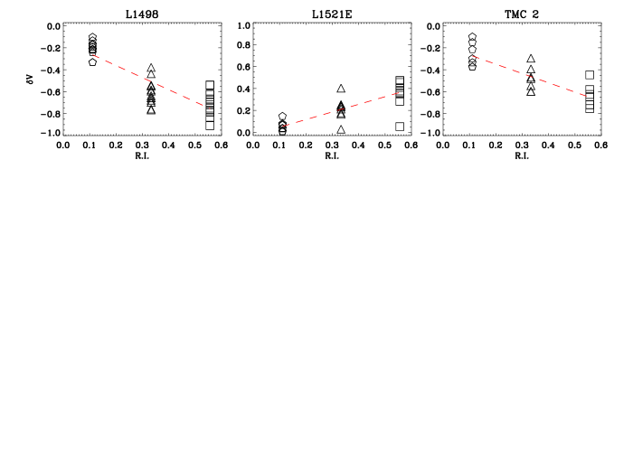
Figure 11: Degree of skewness as a function of the relative intensities of the hyperfine components of HCN(1$-$0). Linear regressions emphasise the relationship between $\delta V$ and line strength (dashed red lines). Values of $\delta V$ from observations of the $F=1\rightarrow 1$ component (triangles), the $F=2\rightarrow 1$ component (squares), and the $F=0\rightarrow 1$ component (pentagons).

6 Excitation temperature results

Even though real deviations from LTE populations are present (see Appendix A), the LTE assumption is an approximation which is useful for many purposes and we calculated the excitation temperature, $T_{\rm ex}$, from a simultaneous LTE fit of the hyperfine components in the observed species, using the measured intensity of optically thick transitions. The main-beam temperature is given by

$$T_{\rm mb}=f_{\rm B}[J_{\nu}(T_{\rm ex})-J_{\nu}(T_{\rm bb})](1-e^{-\tau})\,,$$ (2)

where $J_{\nu}(T)=T_{0}/[\exp(T_{0}/T)-1]$ is the Planck-corrected brightness temperature and $T_{\rm bb}=2.73$ K is the temperature of the cosmic background. $T_{0}\equiv h\nu/k$, where $\nu$ is the transition frequency, and $h$ and $k$ represent Planck’s and Boltzmann’s constants, respectively. If both the source and the beam are Gaussian shaped, the beam filling factor, $f_{\rm B}$, is given by

$$f_{\rm B}=\frac{\Omega_{\rm S}}{\Omega_{\rm B}+\Omega_{\rm S}}\,,$$ (3)

where $\Omega_{\rm B}=1.133\theta_{\rm B}^{2}$ and $\Omega_{\rm S}=1.133\theta_{\rm S}^{2}$ denote the solid angles covered by the beam and the source, respectively, while $\theta_{\rm B}$ and $\theta_{\rm S}$ are the half-power beamwidth of the beam and the source, respectively, this latter evaluated by taking the line intensities stronger than the 50% of the peak value. We found $f_{\rm B}$ to be equal to unity for most of the tracers, because $\Omega_{\rm S}$ is at least one order of magnitude greater than $\Omega_{\rm B}$, except for H¹³CN and HN¹³C in L1521E ($f_{\rm B}=0.88$).

The correct determination of the excitation temperature for HN¹³C and H¹³CN is fundamental. In fact, the gas density of the source sample ($\sim 10^{5}$ cm^-3, see Tafalla et al. 2004a , Tafalla & Santiago 2004b , and Crapsi et al. cc05 (2005) for L1498, L1521E, and TMC 2, respectively) corresponds to a region where the $T_{\rm ex}$ of the two isotopologues changes rapidly with density, namely between the radiation- and collision-dominated density ranges. We can thus in principle use our $T_{\rm ex}$ determinations to constrain the density and temperature in the region where the H¹³CN and HN¹³C lines are formed. Since these transitions are emitted in the region where CO is depleted (see Sect. 4), we gain information about the high density “core of the core”. It is worth noting that our observations also are a test of the collisional rates for HCN and HNC (Sarrasin et al. sa10 (2010), Dumouchel et al. df10 (2010)). We illustrate this in the next section.

6.1 Comparison of observed and expected excitation temperature

In Fig. 12, we show the comparison between the values of the excitation temperatures of H¹³CN and HN¹³C evaluated from the simultaneous fit of the hyperfine components for the three sources examined, revealing that $T_{\rm ex}$(HN¹³C) is essentially always greater than $T_{\rm ex}$(H¹³CN) which we presume to be due to the differing collisional rates. In the same plot, two curves trace the values for $T_{\rm ex}$ computed using RADEX (van der Tak et al. vdtb07 (2007)) which uses the new collisional rates for HNC (Sarrasin et al. sa10 (2010), Dumouchel et al. df10 (2010)) that are no longer assumed equal to HCN. These curves assume kinetic temperatures, $T_{\rm kin}$, equal to 6 and 10 K, and typical values of $2\times 10^{12}$ cm^-2 and 0.2 km s^-1 for column density and line width, respectively. We also assumed that the species are cospatial and hence come from regions of the same kinetic temperature. Notice that we rely on the fact that these lines are not too optically thick and thus $T_{\rm ex}$ determinations are relatively insensitive to column density and line width. We notice an impressive good agreement between theory and observations, even if L1498 shows values a little below the expected theoretical trend.

For L1498, we conclude from the RADEX results that the observed $T_{\rm ex}$ are consistent with a density of a few times 10⁴ cm^-3 but this estimate is sensitive to the assumed temperature. If the kinetic temperature is 10 K, then we can exclude densities as high as 10⁵ cm^-3 in the region where H¹³CN and HN¹³C are undepleted. On the other hand, for a temperature of 6 K, such densities are possible. Clearly, more sophisticated models are needed to break this degeneracy. In general, our results are consistent with the conclusion of Tafalla et al. (tm06 (2006)) that the HCN-HNC “hole” is smaller than that seen in CO isotopologues. This suggests that some CO, but much less than the canonical abundance of about 10^-4, is present in the CO depleted region to supply carbon for HCN and HNC.

For L1521E and TMC 2, a central kinetic temperature of 6 K seems possible. From dust emission models, they are thought to reach central densities of around $3\times 10^{5}$ cm^-3 (Tafalla & Santiago 2004b , Crapsi et al.  cc05 (2005)) which would correspond to excitation temperatures for H¹³CN and HN¹³C higher than observed if the temperature was as high as 10 K.

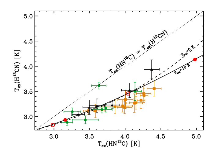
Figure 12: Excitation temperatures of H¹³CN(1$-$0) versus HN¹³C(1$-$0) evaluated from observations of L1498 (yellow squares), L1521E (green circles), and TMC 2 (black triangles). The solid and dashed black lines trace the values for $T_{\rm ex}$ computed using RADEX for kinetic temperatures, $T_{\rm kin}$, of 6 and 10 K; red empty circles and red solid circles show temperatures where number density assumes values equal to 10⁴ and 10⁵ cm^-3 for $T_{\rm kin}=6$ K and 10 K, respectively. The dotted black line depicts the positions where the two excitation temperatures would be equal.

In Fig. 13, we show the observed excitation temperature of HN¹³C and H¹³CN against the H₂ column density inferred from the dust emission. In all the three sources, one notes a clear correlation between $T_{\rm ex}$ and $N$(H₂). This is an important confirmation of the hypothesis that $T_{\rm ex}$ is a measure of collisional rates and that the dust emission peak is also a peak in hydrogen number density. It is also noteworthy that in TMC 2, which has the largest central column density of our three sources, the excitation temperatures continue to increase up to column densities of $8\times 10^{22}$ cm^-2. This suggests that HN¹³C and H¹³CN are still present in the gas phase at densities close to the maximum value in TMC 2 ($3\times 10^{5}$ cm^-3 according to Crapsi et al. cc05 (2005)). On the other hand, the $T_{\rm ex}$ values at the dust peak of TMC 2 are not greatly different from that measured at the dust peak of L1498 suggesting perhaps that the central temperature is lower in TMC 2. In any case, we conclude that excitation temperature determinations of H¹³CN and HN¹³C are a powerful technique for investigating physical parameters towards the density peaks of cores.

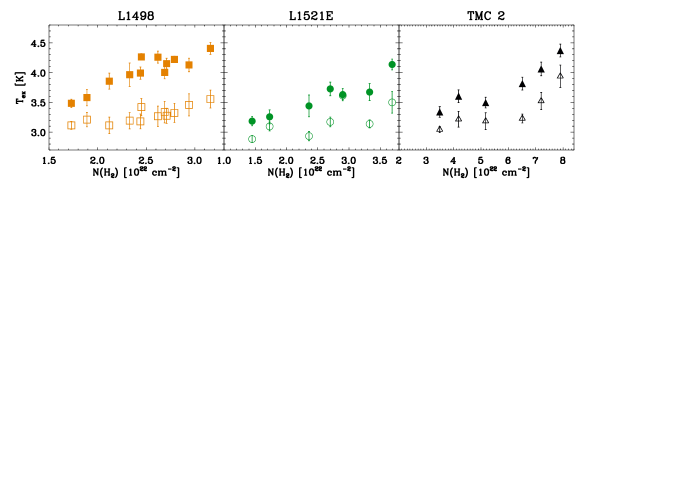
Figure 13: Excitation temperatures of H¹³CN(1$-$0) and HN¹³C(1$-$0), empty and solid points, respectively, as a function of the molecular hydrogen column density from observations of L1498 (yellow squares), L1521E (green circles), and TMC 2 (black triangles).

6.2 Monte Carlo treatment of radiative transfer in L1498

L1498 has been already extensively studied in molecular lines (Tafalla et al. 2004a , tm06 (2006), Padovani et al. pw09 (2009)) and we used the Monte Carlo radiative transfer code in Tafalla et al. (tm02 (2002)) to model H¹³CN and HN¹³C exploiting the recent collisional rate calculations (Sarrasin et al. sa10 (2010), Dumouchel et al. df10 (2010)). The core model is the same as the one used in the analysis of the molecular survey of L1498 published in Tafalla et al. (tm06 (2006)). The core has a density distribution derived from the dust continuum map and an assumed constant gas temperature of 10 K, as suggested by the ammonia analysis. The radiative transfer is solved with a slightly modified version of the Monte Carlo model from Bernes (b79 (1979)). The molecular parameters were taken from the LAMDA database, where the rates are computed for collisions with He and we assumed that the H₂ rates are larger than the He rates by a factor of 2, the same criterion being used for HCN in Tafalla et al. (tm06 (2006)).

With regard to H¹³CN, Tafalla et al. (tm06 (2006)) made use of the collisional rates of Monteiro & Stutzki (ms86 (1986)) which consider hyperfine structure complemented for higher transitions with those of Green & Thaddeus (gt74 (1974)) for higher $J$. In this model, the abundance law is a step function with an outer value of $1.7\times 10^{-10}$ and a central hole of $8\times 10^{16}$ cm. We ran a model with the same abundance law, but this time using the new LAMDA file for HCN, which does not account for hyperfine structure. To compensate for the lack of hyperfine structure, which spreads the photons in velocity, we broadened the line by increasing the amount of turbulence from 0.075 km s^-1 to 0.2 km s^-1. The upper panel of Fig. 14 shows this alternative model which nicely fits the radial profile of observed H¹³CN intensities and this allows us to conclude that the use of the LAMDA file for HCN without hyperfine structure has little effect on the abundance determination, the result being as good as that of Tafalla et al. (tm06 (2006)).

For HN¹³C, we used the collisional rates for the main isotopologue, HNC. As for H¹³CN, the HNC hyperfine structure is not taken into account, so we set again the parameter relative to the turbulent velocity to 0.2 km s^-1. The lower panel of Fig. 14 shows the observed HN¹³C integrated intensities for two fits: one assumes equal abundances for H¹³CN and HN¹³C, the other assumes that the HN¹³C abundance is 1.2 times that of H¹³CN. These radial profiles suggest an abundance ratio between the two molecules close to 1, with a likelihood of being closer to 1.2 towards the centre.

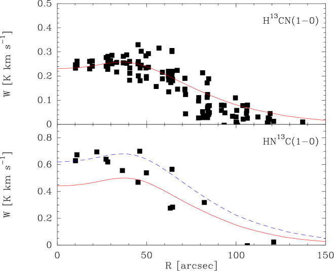
Figure 14: Radial profile of observed H¹³CN(1$-$0) and HN¹³C(1$-$0) integrated intensities (upper and lower panel, respectively) and model prediction for a core with a central hole of $8\times 10^{16}$ cm and an outer abundance value of $1.7\times 10^{-10}$ (red solid lines) and $2.04\times 10^{-10}$ (blue dashed line). HN¹³C(1$-$0) data come from this study and H¹³CN(1$-$0) data come from this study and Tafalla et al. (tm06 (2006)).

The Monte Carlo code also computes the radial profile of excitation temperature, which is presented in the upper panel of Fig. 15. We notice that $T_{\rm ex}$ for both species decreases with the radius from about 4.8 K and 3.8 K for HN¹³C and H¹³CN, respectively, in the core interior, towards the cosmic background temperature near the outer edge of the core. Even more interesting, we found $T_{\rm ex}$(HN¹³C) systematically higher than $T_{\rm ex}$(H¹³CN), in nice agreement with the values computed from observations (see lower panel of Fig. 15 compared with Fig. 12). It is important to stress that $T_{\rm ex}$ values from observations refer to some kind of weighted mean along the line of sight for different positions, while $T_{\rm ex}$ values from Monte Carlo analysis are related to each shell in the core. This means that the two numbers are closely connected, but do not exactly have the same meaning and a proper comparison would require simulating the hyperfine analysis in the Monte Carlo spectra. However, the effect is global over the cloud and affects every layer, so it cannot be ignored in any analysis.

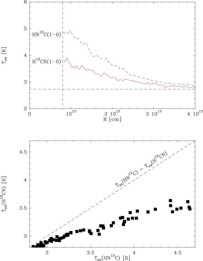
Figure 15: Upper panel: radial profile of excitation temperature for H¹³CN(1$-$0), red solid line, and HN¹³C(1$-$0), blue dashed line, in L1498 as predicted by our best fit Monte Carlo model; the vertical dashed line represents the central hole radius and the horizontal dashed line shows the cosmic background temperature limit. Lower panel: comparison between HN¹³C(1$-$0) and H¹³CN(1$-$0) local values of the excitation temperature in each core shell; the dashed line depicts the positions where the two excitation temperatures would be equal.

7 Column density and abundance estimates

Based on our earlier discussion, HCN hyperfine components are too optically thick to be used for column density determinations. This means that, while H¹³CN, as well as HN¹³C, originate in the central part of the core, HCN is dominated by the foreground layer emission and hence it is not possible to observe the centre of the core. Besides, there is an unequivocal difference between the H¹³CN($F=2\rightarrow 1$) and the HCN($F=0\rightarrow 1$) profiles (see Fig. 9). In fact, H¹³CN seems to be much more Gaussian than the weakest HCN line and it is likely to underestimate the optical depth of HCN.

However, we found that even HN¹³C and H¹³CN are moderately optically thick (see Sect. 3) and in this case one can derive the column density in the $j$th level, $N_{j}$, integrating Eq. (2) over frequency to obtain the integrated intensity, $W_{j}$, with the optical depth given by

$$\tau=\frac{c^{3}}{8\pi\nu_{ji}^{3}}A_{ji}N_{j}(e^{h\nu_{ji}/kT_{\rm ex}}-1)\ \phi(\nu)\,,$$ (4)

where $A_{ji}$ is the Einstein coefficient, and $\phi(\nu)$ the profile function, which is a sum of Gaussians (assuming a maxwellian distribution of the particle velocities) with the appropriate weights and shifts with respect to the central frequency, properly accounting for the hyperfine structure. As shown in Fig. 16, for small optical depths ($\tau<1$) $N_{j}$ is in direct ratio to $W_{j}$ while, as $\tau$ increases, the curve flattens even if the flattening is not very sharp because when the main component is thick, the satellites are still thin. Allowing for increasing optical depth is important not to underestimate column density: as an instance, at the emission peak of H¹³CN in L1498, where $\tau=4.58$ (see Sect. 3), the linear approximation causes an inaccuracy of about 45% and this percentage mainly depends on the optical depth, but not on $T_{\rm ex}$. In fact, for decreasing excitation temperatures, the linear approximation decreases its slope, but also the flattening due to opacity is accentuated. HN¹³C indicates a similar deviation.

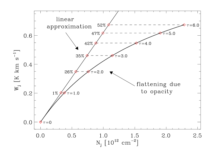
Figure 16: H¹³CN(1$-$0) integrated intensity as a function of the column density of the $J=1$ level for $T_{\rm ex}=3.56$ K (the highest excitation temperature observed in L1498). The percentage values show the deviation of the linear approximation with respect to the correct value taking account for optical depth.

Hence, we determine the column density $N_{j}$ corresponding to the observed $W_{j}$ carrying out this procedure using the maximum and the minimum value of the excitation temperature in order to estimate errors in $N_{j}$. It is important to remark that in this way column densities are directly estimated from the integrated intensity of the spectra, avoiding the use of optical depth values evaluated from the fit of the hyperfine components which have often large uncertainties (see Fig. 4). Finally, for the total column density, $N$, it holds

$$\frac{N_{j}}{N}=\frac{g_{j}}{Q}e^{-E_{j}/kT_{\rm ex}}\,,$$ (5)

where $Q=\Sigma_{j=0}^{\infty}g_{j}\ e^{-E_{j}/kT_{\rm ex}}$ is the partition function, $E_{j}$ and $g_{j}$ being the energy and the statistical weight of the upper $j$th level, respectively.

Hence, we derive the column density and the abundance of these species with respect to molecular hydrogen for the main isotopologues HNC and HCN, assuming the canonical isotopic [¹²C]/[¹³C] ratio (Milam et al. ms05 (2005)). Figure 17 shows HNC and HCN column densities as a function of H₂ column density which has been calculated from the millimetre dust emission, assuming a dust opacity per unit mass of 0.005 cm² g^-1 and a dust temperature of 10 K. Notice the correlation between HNC and HCN column densities and their optical depths in Fig. 4 for L1498: for $N$(H${}_{2})\gtrsim 2.5\times 10^{22}$ cm^-2, $N$(HNC) becomes higher than $N$(HCN) as well as $\tau(\mathrm{HNC})>\tau(\mathrm{HCN})$. Besides, HNC and HCN abundances increase towards the peak in TMC 2 but not in the other two cores.

As an instance, in Table 1 we show the values of column density and abundance with respect to H₂ for HNC and HCN at the dust emission peak.

Figure 17: Column density of HNC(1$-$0), solid squares, and HCN(1$-$0), empty squares for the source sample as a function of the H₂ column density.

Table 1: Column densities and abundances for HNC and HCN at the dust emission peak in our source sample.

source	$N$(HNC)	$N$(HCN)
	[$10^{14}$ cm-2]	[$10^{14}$ cm-2]
L1498	1.58(0.56)	1.24(0.18)
L1521E	0.51(0.14)	0.47(0.12)
TMC 2	2.41(0.42)	1.86(0.26)
	[HNC]/[H2]	[HCN]/[H2]
	[10-9]	[10-9]
L1498	5.00(1.95)	3.92(0.96)
L1521E	1.36(0.42)	1.27(0.37)
TMC 2	3.05(0.57)	2.35(0.36)

From the point of view of the chemistry, it is even more interesting to check the ratio of abundances [HNC]/[HCN] as a function of the column density of molecular hydrogen. Results for the three sources of our sample are showed in Fig. 18.

Figure 18: Abundance ratio [HNC]/[HCN] for the source sample as a function of the H₂ column density.

We found a rather constant value for this ratio, with weighted mean values of $0.94\pm 0.11$ for L1498, $1.14\pm 0.11$ for L1521E, and $1.05\pm 0.10$ for TMC 2, confirming the result achieved by Sarrasin et al. (sa10 (2010)) and Dumouchel et al. (df10 (2010)), and consistent with detailed chemical models available in the literature (e.g. Herbst et al. ht00 (2000)).

This result resolves an important discrepancy between theory and observations which has lasted almost twenty years. There are rather few clear predictions of chemistry theory, but we can confirm that HNC and HCN seem to have similar abundances. However, given that what we measure is the column density of isotopologues, this implies that any fractionation should be the same for the two of them.

Observations of higher-level transitions of HN¹³C and H¹³CN as well as H¹⁵NC and HC¹⁵N would help to refine the determination of column densities and would allow to estimate the isotopic [¹⁴N]/[¹⁵N] ratio, too.

8 Conclusions

We have studied in this article the behaviour of the $J=1\rightarrow 0$ transitions of HCN(1$-$0), H¹³CN(1$-$0), and HN¹³C(1$-$0) as a function of position in the three starless cores L1498, L1521E, and TMC 2. We also observed N₂H⁺(1$-$0) and C¹⁸O(2$-$1) in TMC 2. Our main conclusions are as follows.

• H¹³CN(1$-$0) and HN¹³C(1$-$0) are often assumed to be optically thin when computing column densities. Our results show that in the sources studied by us, this is inaccurate and indeed, optical depths are sufficiently high to make a reasonable estimate of the excitation temperatures of these transitions which can be compared with model predictions.

• The plot of H¹³CN(1$-$0) excitation temperature against HN¹³C(1$-$0) excitation temperature follows the curve expected based on the collision rates recently computed by Sarrasin et al. (2010) and Dumouchel et al. (2010) thus confirming these results. This plot also stresses the importance of calculations of potential surfaces and collisional coefficients for isotopologues separately. Moreover these excitation temperatures correlate well with H₂ column density estimated on the basis of dust emission showing that dust emission peaks really do trace peaks in the gas density.

• These latter results combined with our intensity-offset plots demonstrate convincingly that, at least in TMC 2, HCN and HNC survive in the gas phase at densities above 10⁵ cm^-3 where CO has depleted out. The implication of this is likely that CO survives at abundances of a few percent of its canonical value of around $10^{-4}$ and supplies the carbon required in lower abundance species.

• The profiles of the three satellites of HCN(1$-$0) become increasingly “skew” with increasing optical depth and indeed the corresponding H¹³CN(1$-$0) profiles are reasonably symmetric. This behaviour suggests the possibility of modelling the velocity field and abundance along the line of sight.

• We have used a model of the density distribution in L1498 to describe the HN¹³C(1$-$0) and H¹³CN(1$-$0) results and find reasonable agreement with a model based on the previous observations of Tafalla et al. (2006) containing a central “depletion hole” of radius $8\times 10^{16}$ cm. This does not exclude models without a depletion hole, but does confirm our conclusions on the excitation discussed above. Indeed, rather surprisingly, our results suggest that HN¹³C(1$-$0) and H¹³CN(1$-$0) trace the high density nuclei of these cores when compared with other carbon-bearing species.

• Our results are consistent with the models of Herbst et al. (ht00 (2000)) who found that HNC and HCN should have similar abundances in prestellar cores.

Appendix A Non-LTE hyperfine populations

For a homogeneous slab with LTE between different hyperfine levels, one has

$$R_{ij}=\frac{1-\exp(-f_{i}\tau)}{1-\exp(-f_{j}\tau)},$$ (6)

where $\tau$ is the total transition optical depth and $f_{i}$ is the relative line strength of the $i$th component as in Table 2. We applied this procedure to all the transitions, except for HN¹³C(1$-$0), because of the blending of the hyperfine components. Using the same method adopted in Padovani et al. (pw09 (2009)) for $\mathrm{C_{2}H}$, we consider a homogeneous slab, then a two-layer model, and we compare different couples of ratios one versus the other to quantify the possible departure from LTE. As for $\mathrm{C_{2}H}$, we conclude that also a two-layer model cannot explain the observed intensities, requiring a proper non-LTE treatment.

Comparing the upper and the lower panels of Fig. 19 related to HCN(1$-$0) and H¹³CN(1$-$0), respectively, it is clear that real departures from LTE are present and are stronger in L1498 than in L1521E and TMC 2. In L1498, $R_{32}$, the ratio between the weakest (88633 MHz) and the strongest (88631 MHz) component, is larger than unity and $R_{31}>1$ in all the positions. This suggests a very high self (or foreground) absorption of the strongest component, as found for the C₂H(1$-$0) emission in the same core (Padovani et al. pw09 (2009)). The other two cores show ratios which deviate from the LTE curve revealing again the presence of optical depth effects. As an instance, in the optically thin limit, $R_{32}$ should be equal to about 0.2, but the arithmetic mean of $R_{32}$ is $\sim 0.60$ for L1521E and $\sim 0.47$ for TMC 2.

Finally, an important remark follows from the H¹³CN(1$-$0) ratios (lower panels): minor deviations from LTE are present even in this less abundant isotopologue which should be more optically thin. Even if optically thick lines are the foremost responsible for the arising of non-LTE effects, the density can be high enough to allow transition within the same rotational level (e.g. the transition $J,F=1,2\rightarrow 1,1$ has the same order of magnitude of rates relative to a transition between different rotational levels, see Monteiro & Stutzki, ms86 (1986)).

Figure 19: Ratio of the integrated intensities of couples of components of HCN(1$-$0) (upper panels), and H¹³CN(1$-$0) (lower panels), where $R_{ij}$ represents the ratio between the integrated intensities $W_{i}$ and $W_{j}$ (see Table 2 for component indices). Observational data: L1498 (yellow squares), L1521E (green circles), and TMC 2 (black triangles). One-layer model (black solid curve), two-layer model (magenta dashed curves).

Appendix B Spectroscopic data and observational parameters

Table 2: HCN(1$-$0) and H¹³CN(1$-$0) frequencies of the hyperfine components (From the JPL Molecular Spectroscopy Database: http://spec.jpl.nasa.gov).

Comp no.	$F^{\prime}-F$	Frequency [MHz]	$f$
HCN(1$-$0)
1	1–1	88630.4160	0.333
2	2–1	88631.8470	0.556
3	0–1	88633.9360	0.111
H13CN(1$-$0)
1	1–1	86338.7670	0.333
2	2–1	86340.1840	0.556
3	0–1	86342.2740	0.111

Table 3: HN¹³C(1$-$0) frequencies of the hyperfine components. For a complete list of the hyperfine components, see van Der Tak et al. (vdtm09 (2009)). In fact, there are four overlapped hyperfine components with $F_{2}^{\prime}=2$, three components with $F_{2}^{\prime}=3$, and three components with $F=1\rightarrow 1$.

Comp no.	transition	Frequency [MHz]	$f$
HN13C(1$-$0)
1	$F_{1}^{\prime}-F_{1}=0-1$	87090.675	0.065
2	$\;\;F_{2}^{\prime}=2$	87090.791	0.264
3	$\;\;F_{2}^{\prime}=3$	87090.834	0.432
4	$F_{1}^{\prime}-F_{1}=1-1$	87090.886	0.239

Table 4: Summary of observed molecules together with the observing parameters: half power beamwidth, beam and forward efficiencies, system temperature, and precipitable water vapor.

transition	HPBW	Beff	Feff	Tsys	pwv
	[′′]			[K]	[mm]
HCN(1$-$0)	28	0.77	0.95	$\sim$130	1$-$2
H13CN(1$-$0)	28	0.77	0.95	$\sim$120	1$-$2
HN13C(1$-$0)	28	0.77	0.95	$\sim$140	1$-$2
N2H+(1$-$0)	26	0.77	0.95	$\sim$160	1$-$2
C18O(2$-$1)	11	0.55	0.91	$\sim$320	1$-$2

References

- (1) Akyilmaz, M., Flower, D. R., Hily-Blant, P., Pineau Des Forêts, G. & Walmsley, C. M. 2007, A&A, 462, 221
- (2) Bacmann, A., Lefloch, B., Ceccarelli, C., Castets. A., Steinacker, J. & Loinard, L. 2002, A&A, 389, L6
- (3) Bergin, E. A. & Tafalla, M. 2007, ARA&A, 45, 339
- (4) Bernes, C. 1979, A&A, 73, 67
- (5) Bisschop, S. E., Fraser, H. J., Öberg, K. I., van Dishoeck, E. F. & Schlemmer, S. 2006, A&A, 449, 1297
- (6) Brady Ford, A. & Shirley, Y. L. 2011, ApJ, 728, 144
- (7) Caselli, P., Walmsley, C. M., Zucconi, A., Tafalla, M., Dore, L. & Myers, P. C. 2002a, ApJ, 565, 344
- (8) Caselli, P., Benson, P. J., Myers, P. C. & Tafalla, M. 2002b, ApJ, 572, 238
- (9) Crapsi, A., Caselli, P., Walmsley, C. M., Myers, P. C., Tafalla, M., Lee, C. W. & Bourke, T. L. 2005, ApJ, 619, 379
- (10) Dumouchel, F., Faure, A. & Lique, F. 2010, MNRAS, 406, 2488
- (11) Flower, D. R., Pineau Des Forêts, G. & Walmsley, C. M. 2006, A&A, 456, 215
- (12) Green, S. & Thaddeus, P. 1974, ApJ, 191, 653
- (13) Herbst, E., Terzieva, R. & Talbi, D. 2000, MNRAS, 311, 869
- (14) Hily-Blant, P., Walmsley, C. M., Pineau des Forêts, G. & Flower, D. 2008, A&A, 480, L5
- (15) Hily-Blant, P., Walmsley, C. M., Pineau des Forêts, G. & Flower, D. 2010, A&A, 513, 41 (paper I)
- (16) Mardones, D., Myers, P. C., Tafalla, M., Wilner, D. J., Bachiller, R. & Garay, G. 1997, ApJ, 489, 719
- (17) Milam, S. N., Savage, C., Brewster, M. A., Ziurys, L. M. & Wyckoff, S. 2005, ApJ, 634, 1126
- (18) Monteiro, T. S. & Stutzki, J. 1986, MNRAS, 221, P33
- (19) Padovani, M., Walmsley, C. M., Tafalla, M., Galli, D. & Müller, H. S. P. 2009, A&A, 505, 1199
- (20) Pagani, L., Daniel, F. & Dubernet, M.-L., 2009, A&A, 494, 719
- (21) Pontoppidan, K. M., 2006, A&A, 453, L47
- (22) Sarrasin, E., Abdallah, D. B., Wernli, M., Faure, A., Cernicharo, J. & Lique, F. 2010, MNRAS, 404, 518
- (23) Schmid-Burgk, J., Muders, D., Müller, H. S. P. & Brupbacher-Gatehouse, B. 2004, A&A, 419, 949
- (24) Tafalla, M., Myers, P. C., Caselli, P., Walmsley, C. M. & Comito, C. 2002, ApJ, 569, 815
- (25) Tafalla, M., Myers, P. C., Caselli, P. & Walmsley, C. M. 2004a, A&A, 416, 191
- (26) Tafalla, M. & Santiago, J. 2004b, A&A, 414, L53
- (27) Tafalla, M., Santiago-García, J., Myers, P. C., Caselli, P., Walmsley, C. M. & Crapsi, A. 2006, A&A, 455, 577
- (28) van der Tak, F. F. S., Black, J. H., Schöier, F. L., Jansen, D. J. & van Dishoeck, E. F. 2007, A&A, 468, 627
- (29) van der Tak, F. F. S., Müller, H. S. P., Harding, M. E. & Gauss, J. 2009, A&A, 507, 347
- (30) Walmsley, C. M., Churchwell, E., Nash, A. & Fitzpatrick, E. 1982, ApJ, 258, L75