Entropy of quantum channel in the theory of quantum information

Abstract

Quantum channels, also called quantum operations, are linear, trace preserving and completely positive transformations in the space of quantum states. Such operations describe discrete time evolution of an open quantum system interacting with an environment. The thesis contains an analysis of properties of quantum channels and different entropies used to quantify the decoherence introduced into the system by a given operation.

Part I of the thesis provides a general introduction to the subject. In Part II, the action of a quantum channel is treated as a process of preparation of a quantum ensemble. The Holevo information associated with this ensemble is shown to be bounded by the entropy exchanged during the preparation process between the initial state and the environment. A relation between the Holevo information and the entropy of an auxiliary matrix consisting of square root fidelities between the elements of the ensemble is proved in some special cases. Weaker bounds on the Holevo information are also established.

The entropy of a channel, also called the map entropy, is defined as the entropy of the state corresponding to the channel by the Jamiołkowski isomorphism. In Part III of the thesis, the additivity of the entropy of a channel is proved. The minimal output entropy, which is difficult to compute, is estimated by an entropy of a channel which is much easier to obtain. A class of quantum channels is specified, for which additivity of channel capacity is conjectured.

The last part of the thesis contains characterization of Davies channels, which correspond to an interaction of a state with a thermal reservoir in the week coupling limit, under the condition of quantum detailed balance and independence of rotational and dissipative evolutions. The Davies channels are characterized for one–qubit and one–qutrit systems.

Acknowledgements

I would sincerely like to thank my supervisor Professor Karol Życzkowski for motivation and support in all the time of research and writing of this thesis. I would like to express my gratitude to Professor Mark Fannes for working together on diverse exciting projects. Special thanks to my fellow-worker and friend Fernando de Melo. It is also pleasure to thank Professor Ryszard Horodecki, Professor Paweł Horodecki, Professor Michał Horodecki and Professor Robert Alicki for many opportunities to visit National Quantum Information Centre of Gdańsk and helpful discussions. I would like to show my special gratitude to Professor Tomasz Dohnalik and Professor Jakub Zakrzewski from the Atomic Optics Department for the support and trust in me. I would like to thank my colleagues Piotr Gawron, Zbigniew Puchała, Jarosław Miszczak, Wojciech Bruzda, Łukasz Skowronek and Marek Smaczyński for fruitful collaboration.

Part I Introduction

1 Preliminary information

1.1 Preface

It is not easy to give a satisfactory definition of information in sense in which this word is used in everyday life. For instance one could ask, how much information is contained in an allegorical baroque painting of Vermeer. There exist, of course, many interpretations and therefore, many kinds of information concerning this picture. However, nowadays we are willing to distinguish some sort of information necessary to communicate a message independently on the interpretation. Due to our experience with computers we are used to problems how to encode the information into a string of digital symbols, transmit it and decode it in order to obtain the original message in another place. Imagine that we need to send the information contained in the Vermeer’s picture. We have to encode it into digital data, transmit it to the other place and recover the picture on the screen of the receiver’s computer. In a sense we send almost all the information without knowing what interpretations it may carry.

The problem rises what is the minimal amount of information measured in binary digits that enable the receiver to reliably recover the original message. In considered example we can divide the image of the Vermeer’s picture into small pieces, decode colours of each piece into digital strings and transmit the description of colours one after another. However, we can also save some amount of digits when we menage to describe shapes of regions of the same colours in the picture and send only information about colours, shapes and patterns. How to do that in the most efficient way? This is a major problem for experts working on the information theory and computer graphics. Some rules of the optimal coding were used intuitively during construction of the Morse alphabet. The letters which occur in the English language more frequently are encoded by a smaller amount of symbols.

In communication and computer sciences the problem of data compression is a subject of a great importance. To what extend the data can be compressed to still remain useful? Claude Shannon worked on the problem of transmission of messages through telecommunication channels. In 1958 he published his famous paper [1] opening the new branch of knowledge known as the theory of information. In this theory a message is composed of letters occurring with specified frequencies related to probabilities. Every letter of a message can be encoded as a string of digital units. Every digital unit can appear in one of $r$ possible configurations. Shannon found what is the minimal average amount of digital units per symbol which encodes a given message. This smallest average number of digital units is related to the information contained in the message and is characterized by a function of the probability distribution $P=\{p_{1},...,p_{n}\}$ of letters, now called the Shannon entropy,

$$H(P)=-\sum_{i=1}^{n}p_{i}\log_{r}p_{i},$$ (1)

where $0\log_{r}0\equiv 0$, $n$ is a number of letters and the base of the logarithm $r$ characterizing the amount of configurations of a chosen digital unit can be chosen arbitrary. If the base is equal to $2$, the unit of entropy is called binary unit or bit.

The idea of efficient coding concerns in replacing more frequent letters by means of a smaller amount of bits. Shannon treated the message as a sequence of letters generated independently according to the probability distribution $P$ specified for a given language. The original reasoning of Shannon proceeds as follows. There are so many possible messages as the amount of typical sequences of letters with a given probability distribution in the string of length $k\rightarrow\infty$. Atypical sequences such as strings of letters $a$ repeated $k$ times are unlikely and are not taken into account. The amount of possible messages is given by the amount of typical sequences, which is of order of $2^{kH(P)}$ if the base of the logarithm is equal to 2. This number is justified by methods of combinatorics. Hence, every typical message of length $k$ can be represented by a string of bits of size $kH(P)$. Therefore, the entropy $H(P)$ can be interpreted as the smallest average amount of bits per letter needed to reliably encode each typical message.

The information theory treats, as well, the information as a measure of uncertainty about the outcome of a random experiment. Looking for a function which is suitable as a measure of the uncertainty about the concrete result of experiment, provided the probabilities of all experimental outcomes are given, Shannon formulated a few postulates for the information measure [1]:

• It is a continues function of the probability distribution.

• If all events are equally likely the function of uncertainty is an increasing function of their number.

• If one of the events is split into two, the new function of uncertainty is equal to the sum of the original uncertainty and the uncertainty of the new division weighted by the probability of the divided event.

The only function which satisfies these postulates is the Shannon entropy $H(P)$. Therefore, the uncertainty or lack of information on the outcome of an experiment is the second interpretation of the entropy $H(P)$.

Taking a weaker set of axioms allows one to generalize the definition of the measure of uncertainty and to find other functions of probability vector $P$, which in special case converge to the Shannon entropy (1). For instance, Rényi introduced one parameter family of generalized entropy functions. Since, the information of an experiment consisting of two independent experiments should be given by the sum of the information gained in both experiments, the measure of information should be additive. The Shannon entropy of the joint probability distribution of two independent variables is additive. Rényi noticed [2] that the additivity of information is not equivalent to the third postulate of Shannon. However, if one replaces the third postulate by additivity of information of independent events, yet another axiom should be postulated to obtain back the Shannon’s formula (1). This additional postulate specifies the way of calculating the mean values. If one considers the linear mean, the Shannon entropy is singled out by this set of postulates. However, other definition of the mean value also can be taken. In consequence, the new set of postulates implies an one parameter family of generalized entropy functions known as the Rényi entropy of order $q$:

$$H_{q}(P)=\frac{1}{1-q}\log\sum_{i=1}^{n}p_{i}^{q}.$$ (2)

Here, $q$ denotes the free parameter depending on the definition of the average. Another generalization of entropy function was analysed by Tsallis [3, 4]. The Tsallis entropy of order $q$ is defined as follows,

$$T_{q}=\frac{1}{q-1}(1-\sum_{i}^{n}p_{i}^{q}).$$ (3)

Hence the information theory concerns entropies, however, it also investigates communication sources and communication channels which can introduce some errors to messages. Information theory defines such quantities as the relative entropy and the mutual information [1]. Using these concepts the channel capacity is defined. It is the maximal rate of information which can be reliably decoded after passing through the channel. The channel capacity is measured in bits per a unit of time.

The theory of quantum information, which considers quantum systems as carriers of information, should enable one to generalize the notions of classical information theory such as the channel capacity. To formulate a quantum counterpart of the Shannon concepts such as the relative entropy or channel capacity the theory of open quantum systems, quantum statistical processes, statistical operators, density matrices, partial traces and generalized measurements should be applied. In the early stage of the stochastic theory of open quantum systems, it was developed by Davies [5], and Kossakowski [6]. Moreover, other important results on accessible information transmitted through a noisy quantum channel were obtained by Holevo [7].

There are many advantages of using quantum resources to transform and transmit the information [8]. In particular, there exist a famous protocols of superdense coding [9] of information into a quantum carrier. Furthermore, some computational problems can be solved in framework of the quantum information processing faster than classically [10, 11, 12]. Quantum world gives also new communication protocols like quantum teleportation [9, 13] which is possible due to quantum entanglement [14, 15]. In quantum case, entangled states can increase the joint capacity of two channels with respect to the sum of the two capacities [16, 17, 18]. Also a new branch of cryptography was developed due to the quantum theory [19]. Although, these new possibilities are promising, manipulation of quantum resources is difficult in practice. In particular, the quantum states carrying the information are very sensible to noise, which can completely destroy quantum information. Moreover, probabilistic nature of quantum theory does not allow us to extract uniquely the information from quantum sources. Many restrictions and laws of quantum information theory are formulated in terms of inequalities of quantum entropies. The most significant quantum entropy is the one defined by von Neumann [20, 21], which is a counterpart of the Shannon entropy. However, the other quantum entropies such like the Rényi entropy [2] or Tsallis entropy are also considered [3, 4, 22].

The issue of transmitting a classical information through a noisy channel is an important issue in the information theory [1, 23, 24]. Among problems concerning the information channels one can specify the following questions: How to encode the information in order to transmit it reliably through the channel in the most efficient way [1, 25]? What is the maximal rate of the information transmission? What is the capacity of a given communication channel [26, 27, 28, 29]? Which states are the most resistant to errors occurring in the a channel [30, 31]? What are the efficient strategies of the error correction [32]?

Similar questions can also be formulated in the framework of quantum information theory. The quantum channels, also called quantum operations, are transformations in the set of states [33, 34, 35, 36]. They describe evolution of an open quantum system interacting with an environment in discrete time.

The set of all quantum channels is still not completely understood. Merely the set of one–qubit channels is satisfactory explored [37, 38]. However, even in this simplest case some interesting problems are open. For instance, it is not clear, whether the capacity of one–qubit channels is additive [18]. Another approach to quantum channels suggests to analyse only certain special classes of them, motivated by some physical models [39, 40, 41, 42, 43].

Quantum channels are also formally related to measurement processes in quantum theory [35, 45]. As a measurement process changes the quantum state and in general cannot perfectly distinguish measured states, there is a fundamental restriction on the information which can be obtained from the message encoded into quantum states [7]. These restrictions are also formulated in terms of entropies.

The different aspects of quantum channels mentioned above suggest that entropies which characterize the channels play an important role in the information theory. This thesis is devoted to investigation of quantum channels and some entropies used to characterize them: the minimal output entropy [39, 18], the map entropy [46, 47, 48] and the exchange entropy [29].

1.2 Structure of the thesis

The thesis is partially based on results already published in articles [46, 49, 50, 51, 52, 53], which are enclosed at the end of the thesis. In a few cases some issues from these papers are discussed here in a more detailed manner. The thesis contains also some new, unpublished results and technical considerations not included in the published articles.

The structure of the thesis is the following. The thesis is divided into three parts. The first part is mostly introductory and contains a short review of the literature. This part provides basic information useful in the other parts of the thesis and fixes notation used in the entire work. In part I only the result from Section 1.6.1 concerning the Kraus representation of a complementary channels and Section 1.9 on the Kraus operators constructed for an ensemble of states are obtained by the author.

Part II contains results based on papers [49, 52, 46], not known before in the literature. However, some results not published previously are also analysed there.

Chapter 2 contains the most important result of the thesis – the inequality between the Holevo information related to an ensemble of quantum states and the entropy of the state of environment taking part in preparation of the ensemble. As the entropy of the environment can be treated equivalently as the entropy of an output of the complementary channel, or the entropy of a correlation matrix, or the entropy of a Gram matrix of purifications of mixed states, or as the entropy exchange, this relation might be considered as a new and universal result in the theory of quantum information. Consequences of this inequality have not been analysed so far. Chapter 2 contains also the discussion of the particular cases for which the inequality is saturated. This result has not been published before. Section 2.1 describes proofs of known entropic inequalities which are related to the bound on the Holevo quantity. Some new and unpublished consequences of these inequalities are presented in Section 2.1.1. Original, new results are also contained in Sections 2.2 and 2.3.

Part II contains, moreover, the conjecture on the inequality between the Holevo information of a quantum ensemble and the entropy of the matrix of square root of fidelities. Several weaker inequalities are analysed here in a greater detail than it was done in [52]. Section 3.2 presents a confirmation of the conjecture for a special class of ensembles of quantum states.

Part III of the thesis is based on the results presented in [51, 50]. Article [51] described partially in Chapter 4 considers the relation between minimal output entropy and the map entropy. Section 4.2 contains a proof of additivity of the map entropy with respect to the tensor product of two maps, already published in our work [51]. These results allow us to specify a class of quantum channels for which additivity of the minimal output entropy is conjectured.

The Davies maps acting on one–qubit and one–qutrit quantum systems are analysed in Chapter 5. Conditions for the matrix entries of a quantum operation representing a Davies map are given along the lines formulated in our work [50]. Multiplicativity of the maximal output norm of one–qubit Davies maps, entirely based on the analogical proof for bistochastic maps [54], is presented in Section 5.6. However, this result cannot be treated as a new one, since multiplicativity of the maximal output two norm was proved earlier for all one–qubit quantum channels [18]. Section 5.7 contains graphical representations of stochastic matrices of order three which correspond to quantum Davies maps, which has not been published yet.

1.3 A short introduction to quantum mechanics

The formalism of quantum mechanics can be derived from a few postulates (axioms) which are justified by experiments. The set of axioms defining the quantum theory differs depending on the author [55]. However, some features occur common in every formulation, either as axioms or as their consequences. One of such key features is the superposition principle. It is justified by several experimental data as interference pattern in double slit experiment with electrons or interference of a single photon in the Mach–Zender interferometer [56]. The superposition principle states that the state of a quantum system, which is denoted in Dirac notation by $|\psi\rangle$, can be represented by a coherent combination of several states $|\psi_{i}\rangle$ with complex coefficients $a_{i}$,

$$|\psi\rangle=\sum_{i}a_{i}|\psi_{i}\rangle.$$ (4)

The quantum state $|\psi\rangle$ of an $N$ level system is represented by a vector from the complex Hilbert space $\mathcal{H}_{N}$. The inner product $\langle\psi_{i}|\psi\rangle$ defines the coefficients $a_{i}$ in (4). The square norm of $a_{i}$ is interpreted as the probability that the system described by $|\psi\rangle$ is in the state $|\psi_{i}\rangle$. To provide a proper probabilistic interpretation a vector used in quantum mechanics is normalized by the condition $\langle\psi|\psi\rangle=||\psi||^{2}=\sum_{i}|a_{i}|^{2}=1$.

Quantum mechanics is a probabilistic theory. One single measurement does not provide much information on the prepared system. However, several measurements on identically prepared quantum systems allow one to characterize the quantum state.

A physical quantity is represented by a linear operator called an observable. An observable $A$ is a Hermitian operator, $A=A^{\dagger}$, which can be constructed by a set of real numbers $\lambda_{i}$ (allowed values of the physical quantity) and a set of states $|\varphi_{i}\rangle$ determined by the measurement, $A=\sum_{i}\lambda_{i}|\varphi_{i}\rangle\langle\varphi_{i}|$. The physical value corresponds to the average of the observable in the state $|\psi\rangle$,

$$\langle A\rangle_{\psi}=\sum_{i}\lambda_{i}|\langle\psi|\varphi_{i}\rangle|^{2}=\langle\psi|A|\psi\rangle.$$ (5)

One can consider the situation in which a state $|\psi\rangle$ is not known exactly. Only a statistical mixture of several quantum states $|\phi_{i}\rangle$ which occur with probabilities $p_{i}$ is given. In this case the average value of an observable has the form

$$\langle A\rangle_{\{p_{i},\phi_{i}\}}=\sum_{i}p_{i}\langle\phi_{i}|A|\phi_{i}\rangle,$$ (6)

which can be written in terms of an operator on $\mathcal{H}_{N}$ called a density matrix $\rho=\sum_{i}p_{i}|\phi_{i}\rangle\langle\phi_{i}|$ as

$$\langle A\rangle_{\{p_{i},\phi_{i}\}}=\operatorname*{Tr}\rho A.$$ (7)

A density matrix describes a so called mixed state. In a specific basis the density matrices characterizing an $N$ level quantum system are represented by $N\times N$ matrices $\rho$ which are Hermitian, have trace equal to unity and are positive. Let us denote the set of all such matrices by $\mathcal{M}_{N}$,

$$\mathcal{M}_{N}=\{\rho:{\rm dim}\rho=N,\rho=\rho^{\dagger},\rho\geq 0,\operatorname*{Tr}\rho=1\}.$$ (8)

This set is convex. Extremal points of this set are formed by projectors of the form $|\psi\rangle\langle\psi|$ called pure states, which correspond to vectors $|\psi\rangle$ of the Hilbert space.

The state of composed quantum system which consists of one $N_{1}$–level system and one $N_{2}$–level system is represented by a vector of size $N_{1}N_{2}$ from the Hilbert space which has a tensor product structure, $\mathcal{H}_{N_{1}N_{2}}=\mathcal{H}_{N_{1}}\otimes\mathcal{H}_{N_{2}}$. Such a space contains also states which cannot be written as tensor products of vectors from separate spaces,

$$|\psi_{12}\rangle\neq|\psi_{1}\rangle\otimes|\psi_{2}\rangle.$$ (9)

and are called entangled states. States with a tensor product structure are called product states. If the state of only one subsystem is considered one has to take an average over the second subsystem. Such an operation is realized by taking the partial trace over the second subsystem and leads to a reduced density matrix,

$$\rho_{1}={\rm Tr}_{2}\rho_{12}.$$ (10)

A density matrix describes therefore the state of an open quantum system.

The evolution of a normalized vector in the Hilbert space is determined by a unitary operator $|\psi^{\prime}\rangle=U|\psi\rangle$. The transformation $U$ is related to Hamiltonian evolution due to the Schrödinger equation,

$$i\hbar\frac{d}{dt}|\psi\rangle=H|\psi\rangle,$$ (11)

where $H$ denotes the Hamiltonian operator of the system, while $t$ represents time and $2\pi\hbar$ is the Planck constant. A discrete time evolution of an open quantum system characterized by a density operator $\rho$ is described by a quantum operation which will be considered in Chapter 1.6.

According to a general approach to quantum measurement [35, 57], it can be defined by a set of $k$ operators $\{E^{i}\}_{i=1}^{k}$ forming a positive operator valued measure (POVM). The index $i$ is related to a possible measurement result, for instance the value of the measured quantity. The operators $E^{i}$ are positive and satisfy the identity resolution,

$$\sum_{i=1}^{k}E^{i}={\rm 1\rule{0.43057pt}{6.54443pt}\hskip 0.86108pt}.$$ (12)

The quantum state is changing during the measurement process. After the measurement process that gives the outcome $i$ as a result, the quantum state $\rho$ is transformed into

$$\rho^{\prime}_{i}=K^{i}\rho K^{i\dagger}/\operatorname*{Tr}(K^{i}\rho K^{i\dagger}),$$ (13)

where $K^{i\dagger}K^{i}=E^{i}\geq 0$. The probability $p_{i}$ of the outcome $i$ is given by $p_{i}=\operatorname*{Tr}(K^{i}\rho K^{i\dagger})$. Due to relation (12), the probabilities of all outcomes sum up to unity.

A quantum state characterizing a $2$–level system is called qubit and its properties are discussed in more detail in Section 1.7.

1.4 Schmidt decomposition

The theorem known as Schmidt decomposition [58] provides a useful representation of a pure state of a bi–partite quantum system.

Theorem 1 (Schmidt).

Any quantum state $|\psi_{12}\rangle$ from the Hilbert space composed of the tensor product of two Hilbert spaces $\mathcal{H}_{1}\otimes\mathcal{H}_{2}$ of dimensions $d_{1}$ and $d_{2}$, respectively, can be represented as

$$|\psi_{12}\rangle=\sum_{i=1}^{d}\lambda_{i}|i_{1}\rangle\otimes|i_{2}\rangle,$$ (14)

where $\{|i_{1}\rangle\}_{i=1}^{d_{1}}$ and $\{|i_{2}\rangle\}_{i=1}^{d_{2}}$ are orthogonal basis of the Hilbert spaces $\mathcal{H}_{1}$ and $\mathcal{H}_{2}$ respectively, and $d=\min\{d_{1},d_{2}\}$.

Proof.

Choose any orthogonal basis $\{|\phi^{k}_{1}\rangle\}_{k=1}^{d_{1}}$ of $\mathcal{H}_{1}$ and any orthogonal basis $\{|\phi^{j}_{2}\rangle\}_{j=1}^{d_{2}}$ of $\mathcal{H}_{2}$. In this product basis, the bi–partite state $|\psi_{12}\rangle$ reads

$$|\psi_{12}\rangle=\sum_{0\leq k\leq d_{1},\ 0\leq j\leq d_{2}}a_{kj}|\phi^{k}_{1}\rangle\otimes|\phi^{j}_{2}\rangle.$$ (15)

Singular value decomposition of a matrix $A$ of size $d_{1}\times d_{2}$ with entries $a_{kj}$ gives $a_{kj}=\sum_{i}u_{ki}\lambda_{i}v_{ij}$. Here $u_{ki}$ and $v_{ij}$ are entries of two unitary matrices, while $\lambda_{i}$ are singular values of $A$. Summation over indexes $k$ and $j$ cause changes of two orthogonal bases into

$$|i_{1}\rangle=\sum_{k}u_{ki}|\phi^{k}_{1}\rangle,$$ (16)

$$|i_{2}\rangle=\sum_{j}v_{ij}|\phi^{j}_{2}\rangle.$$ (17)

The number o nonzero singular values is not larger than the smaller one of the numbers $(d_{1},d_{2})$. ∎

The Schmidt decomposition implies that both partial traces of any bi–partite pure state have the same nonzero part of the spectrum:

$${\rm Tr}_{1}|\psi_{12}\rangle\langle\psi_{12}|=\sum_{i=1}^{d}\lambda_{i}^{2}|i_{2}\rangle\langle i_{2}|,$$ (18)

$${\rm Tr}_{2}|\psi_{12}\rangle\langle\psi_{12}|=\sum_{i=1}^{d}\lambda_{i}^{2}|i_{1}\rangle\langle i_{1}|.$$ (19)

The Schmidt coefficients $\lambda_{i}$ are invariant under local unitary transformations $U_{1}\otimes U_{2}$ applied to $|\psi_{12}\rangle$. The number of non–zero coefficients $\lambda_{i}$ is called the Schmidt number. Any pure state which has the Schmidt number greater than 1 is called entangled state. A pure state for which all Schmidt coefficients $\lambda_{i}$ are equal to $1/\sqrt{d}$ is called a maximally entangled state.

Another important consequence of the Schmidt decomposition is that for any mixed state $\rho$ there is a pure state $|\psi\rangle$ of a higher dimensional Hilbert space such that $\rho$ can be obtained by taking the partial trace,

$$\rho={\rm Tr}_{1}|\psi\rangle\langle\psi|.$$ (20)

Such a state $|\psi\rangle$ is called a purification of $\rho$. The Schmidt decomposition gives the recipe for the purification procedure. It is enough to take square roots of eigenvalues of $\rho$ in place of $\lambda_{i}$ and its eigenvectors in place of $|i_{1}\rangle$. Any orthogonal basis in $\mathcal{H}_{2}$ provides a purification of $\rho$, which can be written as

$$|\psi\rangle=\sum_{i}(U_{1}\otimes\sqrt{\rho})|i_{1}\rangle\otimes|i_{2}\rangle,$$ (21)

where $U_{1}$ is an arbitrary unitary transformation and $\sqrt{\rho}|i_{2}\rangle=\lambda_{i}|i_{2}\rangle$.

1.5 Von Neumann entropy and its properties

Many theorems concerning the theory of quantum information can be formulated in terms of the von Neumann entropy [59] of a quantum state,

$$S(\rho)=-\operatorname*{Tr}\rho\log\rho,$$ (22)

which is equivalent to the Shannon entropy (1) of the spectrum of $\rho$. The entropy characterizes the degree of mixing of a quantum state. Assume that $\rho$ is a density matrix of size $N$. The value of $S(\rho)$ is equal to zero if and only if the state $\rho$ is pure. It gains its maximal value $\log N$ for the maximally mixed state $\rho_{*}=\frac{1}{N}{\rm 1\rule{0.43057pt}{6.54443pt}\hskip 0.86108pt}$ only.

Von Neumann entropy has also an important interpretation in quantum information theory, as it plays the role similar to the Shannon entropy in the classical theory of optimal compression of a message [25]. Let the letters $i$ of the message, which occur with probabilities $p_{i}$, be encoded into pure quantum states $|\psi_{i}\rangle$ from the Hilbert space $\mathcal{H}_{N}$. Sequences of $k$ letters are encoded into a Hilbert space of dimension $N^{k}$. A long message can be divided into sequences of size $k\rightarrow\infty$. Among them one can distinguish sequences in typical subspaces and such which occur with negligible probability. A unitary transformation applied to the sequence of quantum systems can transmit almost all the information into a typical subspace. The space of a typical sequence has the smallest dimensionality required to encode the message reliably with negligible probability of an error. This smallest dimensionality per symbol is shown [25] to be equal to the von Neumann entropy of the state $\rho=\sum_{i}p_{i}|\psi_{i}\rangle\langle\psi_{i}|$. Therefore, quantum coding consists in taking states from the smaller subspace of dimension $2^{kS(\rho)}$ instead of a space of dimension $N^{k}$ to encode the same message. If the state $\rho$ represents completely random set of states there is no possibility to compress the message, since $S(\rho)=S(\rho_{*})=\log_{2}N$, where logarithm is of base 2. The entropy, therefore, describes the capability of compression of the message encoded in a given set of states, or the smallest amount of qubits needed to transmit a given message.

The von Neumann entropy, as the entropy of eigenvalues of a density matrix, describes also the uncertainty of measuring a specific state from the set of the eigenvectors. The most important properties of the von Neumann entropy are [20]:

• The von Neumann entropy is a non negative function of any $\rho$.

• It is invariant under unitary transformations, $S(\rho)=S(U\rho U^{\dagger})$.

• It is a concave function of its argument, $\sum_{i=1}^{k}p_{i}S(\rho_{i})\leq S(\sum_{i=1}^{k}p_{i}\rho_{i})$, where $p_{i}\geq 0$ for any $i$ and $\sum_{i}^{k}p_{i}=1$.

• It is subadditive

  $$S(\rho_{12})\leq S(\rho_{1})+S(\rho_{2}),$$ (23)

  where $\rho_{12}$ is a bi–partite state of a composite system and the partial traces read $\rho_{1}=\operatorname*{Tr}_{2}\rho_{12}$ and $\rho_{2}=\operatorname*{Tr}_{1}\rho_{12}$.

• The von Neumann entropy satisfies the relation of strong subadditivity [60],

  $$S(\rho_{123})+S(\rho_{2})\leq S(\rho_{12})+S(\rho_{23}),$$ (24)

  where the state $\rho_{123}$ is a composite state of three subsystems $(1,2,3)$ and the other states are obtained by its partial traces.

1.6 Quantum channels and their representations

One distinguishes two approaches to describe time evolution of an open quantum system. One of them starts from a concrete physical model defined by a given Hamiltonian which determines the Shrödinger equation (11) or the master equation, [45]. Solving them one may find the state of the quantum system at any moment at time. An alternative approach to the dynamics of an open quantum system relies on a stroboscopic picture and a discrete time evolution. It starts from a mathematical construction of a quantum map, $\rho^{\prime}=\Phi(\rho)$, allowed by the general laws of quantum mechanics. This approach is often used in cases in which the physical model of the time evolution is unknown. This fact justifies the name "black box" model to describe the evolution characterized by a quantum map $\Phi$. Such a model is also considered if one wants to investigate the set of all possible operations independently on whether the physical context is specified. Main features and some representations of the map $\Phi$, which describes a "black box" model of non–unitary quantum evolution, are given below.

The quantum map $\Phi$ describes the dynamics of a quantum system $\rho$ which interacts with an environment. It is given by a nonunitary quantum map $\Phi:\rho\rightarrow\rho^{\prime}$. Any such map is completely positive, and trace preserving [33, 34, 35, 36]. "Complete positivity" means that an extended map $\Phi\otimes{\rm 1\rule{0.43057pt}{6.54443pt}\hskip 0.86108pt}_{M}$, which is a trivial extension of $\Phi$ on the space of any dimension $M$, transforms the set of positive operators into itself. A completely positive and trace preserving quantum map is called quantum operation or quantum channel.

Due to the theorem of Jamiołkowski [34] and Choi [33] the complete positivity of a map is equivalent to positivity of a state corresponding to the map by the Jamiołkowski isomorphism. This isomorphism determines the correspondence between a quantum operation $\Phi$ acting on $N$ dimensional matrices and density matrix $D_{\Phi}/N$ of dimension $N^{2}$ which is called Choi matrix or the Jamiołkowski state

$$\frac{1}{N}D_{\Phi}=[\operatorname{id}_{N}\otimes\Phi]\big{(}|\phi^{+}\left.\right\rangle\left\langle\right.\phi^{+}|\big{)},$$ (25)

where $|\phi^{+}\left.\right\rangle=\frac{1}{\sqrt{N}}\sum_{i=1}^{N}|i\left.\right\rangle\otimes|i\left.\right\rangle$ is a maximally entangled state. The dynamical matrix $D_{\Phi}$ corresponding to a trace preserving operation satisfies the partial trace condition

$${\rm Tr}_{2}D_{\Phi}={\rm 1\rule{0.43057pt}{6.54443pt}\hskip 0.86108pt}.$$ (26)

The quantum operation $\Phi$ can be represented as superoperator matrix. It is a matrix which acts on the vector of length $N^{2}$, which contains the entries $\rho_{ij}$ of the density matrix ordered lexicographically. Thus the superoperator $\Phi$ is represented by a square matrix of size $N^{2}$. The superoperator in some orthogonal product basis $\{|i\rangle\otimes|j\rangle\}$ is represented by a matrix indexed by four indexes,

$$\Phi_{\!\!\!\!\footnotesize{\begin{array}[]{cc}i&\!\!\!\!\!\!j\\ k&\!\!\!\!\!\!l\end{array}}}=\langle i|\otimes\langle j|\Phi|k\rangle\otimes|l\rangle.$$ (27)

The matrix representation of the dynamical matrix is related to the superoperator matrix by the reshuffling formula [15] as follows

$$\langle i|\otimes\langle j|D_{\Phi}|k\rangle\otimes|l\rangle=\langle i|\otimes\langle k|\Phi|j\rangle\otimes|l\rangle.$$ (28)

To describe a quantum operation, one may use the Stinespring’s dilation theorem [61]. Consider a quantum system, described by the state $\rho$ on $\mathcal{H}_{N}$, interacting with its environment characterized by a state on $\mathcal{H}_{M}$. The joint evolution of the two states is described by a unitary operation $U$. Usually it is assumed that the joint state of the system and the environment is initially not entangled. Moreover, due to the possibility to purification the environment, its initial state is given by a pure one. The evolving joint state is therefore:

$$\omega=U\Big{(}\left|1\right\rangle\left\langle 1\right|\otimes\rho\Big{)}U^{\dagger},$$ (29)

where $|1\rangle\in\mathcal{H}_{M}$ and $U$ is a unitary matrix of size $NM$. The state of the system after the operation is obtained by tracing out the environment,

$$\rho^{\prime}=\Phi(\rho)={\rm Tr}_{M}\Big{[}U\big{(}\left|1\right\rangle\left\langle 1\right|\otimes\rho\big{)}U^{\dagger}\Big{]}=\sum_{i=1}^{M}K^{i}\rho K^{i\dagger},$$ (30)

where the Kraus operators read, $K^{i}=\left\langle i\right|U\left|1\right\rangle$. In matrix representation the Kraus operators are formed by successive blocks of the first block–column of the unitary evolution matrix $U$. Here the state $\omega$ can be equivalently given as

$$\omega=\sum_{i,j=1}^{M}K^{i}\rho K^{j\dagger}\otimes\left|i\right\rangle\left\langle j\right|.$$ (31)

A transformation $\rho\rightarrow\omega$ is obtained by an isometry $F:\mathcal{H}_{N}\rightarrow\mathcal{H}_{NM}$, where

$$F\left|\phi\right\rangle=\sum_{i}(K^{i}\left|\phi\right\rangle)\otimes\left|i\right\rangle.$$ (32)

Due to the Kraus theorem [35] any completely positive map $\Phi$ can be written in the Kraus form,

$$\rho^{\prime}=\Phi(\rho)=\sum_{i=1}^{M}K^{i}\rho K^{i\dagger}.$$ (33)

The opposite relation is also true, any map of the Kraus form (33) is completely positive.

1.6.1 Representation of a complementary channel

Consider a quantum channel $\Phi$ described by the Kraus operators $K^{i}$,

$$\Phi(\rho)={\rm Tr}_{M}\omega=\sum_{i=1}^{M}K^{i}\rho K^{i\dagger},$$ (34)

where notation from Section 1.6 is used. The channel $\tilde{\Phi}$ complementary to $\Phi$ is defined by

$$\tilde{\Phi}(\rho)={\rm Tr}_{N}\omega=\sum_{i=1}^{N}\tilde{K}^{i}\rho\tilde{K}^{i\dagger}$$ (35)

and it describes the state of the $M$–dimensional environment after the interaction with the principal system $\rho$. One can derive the relation between operators $\{\tilde{K}^{j}\}_{j=1}^{N}$ and $\{K^{i}\}_{i=1}^{M}$ from the last equation by substituting $\omega$ as in (31). This relation can be rewritten as

$$\sum_{i,j=1}^{M}(\operatorname*{Tr}K^{i}\rho K^{j\dagger})\left|i\right\rangle\left\langle j\right|=\sum_{i=1}^{N}\tilde{K}^{i}\rho\tilde{K}^{i\dagger}.$$ (36)

Comparison of the matrix elements of both sides gives

$$\sum_{\alpha=1}^{N}\tilde{K}^{\alpha}_{im}\rho_{mn}\tilde{K}^{\alpha\dagger}_{nj}=\sum_{\alpha=1}^{N}K^{i}_{\alpha m}\rho_{mn}K^{j\dagger}_{n\alpha},$$ (37)

where matrix elements are indicated by lower indexes and the Einstein summation convention is applied. Hence, for any quantum channel $\Phi$ given by a set of Kraus operators $K^{i}$, one can define the Kraus operators $\tilde{K}^{\alpha}$ representing the complementary channel $\tilde{\Phi}$ as

$$\tilde{K}^{\alpha}_{ij}=K^{i}_{\alpha j},\qquad i=1,...,M,\qquad j,\alpha=1,...,N.$$ (38)

1.7 One–qubit channels

One–qubit channels acting on density matrices of size $2$ have many special features which cause that the set of these channels is well understood [37, 38, 54]. However, many properties of one–qubit maps are not shared with the quantum maps acting on higher dimensional systems. Since one–qubit quantum channels are often considered in this thesis, the following section presents a brief review of their basic properties.

A quantum two level state is called quantum bit or qubit. It is represented by a $2\times 2$ density matrix. Any Hermitian matrix of size two can be represented in the basis of identity matrix and the three Pauli matrices $\vec{\sigma}=\{\sigma_{1},\sigma_{2},\sigma_{3}\}$,

$$\sigma_{1}=\begin{pmatrix}0&1\\ 1&0\end{pmatrix},\qquad\sigma_{2}=\begin{pmatrix}0&-i\\ i&0\end{pmatrix},\qquad\sigma_{3}=\begin{pmatrix}1&0\\ 0&-1\end{pmatrix}.$$ (39)

One qubit state $\rho$ decomposed in the mentioned basis is given by the formula

$$\rho=\frac{1}{2}(\operatorname{id}+{\vec{r}}\cdot\vec{\sigma}),\quad{\vec{r}}\in\mathbbm{R}^{3}.$$ (40)

Positivity condition, $\rho\geq 0$, implies that $|\vec{r}|\leq 1$. The vector $\vec{r}$ is called the Bloch vector. All possible Bloch vectors representing quantum states form the Bloch ball. Pure one–qubit states form a sphere of radius $|\vec{r}|=1$.

Any linear one–qubit quantum operation $\Phi$ transforms the Bloch ball into the ball or into an ellipsoid inside the ball. The channel $\Phi$ transforms the Bloch vector $\vec{r}$ representing the state $\rho$ into $\vec{r}\,^{\prime}$ which corresponds to $\rho^{\prime}$. This transformation is described by

$$\vec{r}\,^{\prime}=W\vec{r}+\vec{\kappa}.$$ (41)

Here the matrix $W$ is a square real matrix of size $3$. A procedure analogous to the singular value decomposition of the matrix $W$ gives $W=O_{1}DO_{2}$, where $O_{i}$ represents an orthogonal rotation and $D$ is diagonal. Up to two orthogonal rotations, one before the transformation $\Phi$ and one after it, the one–qubit map $\Phi$ can be represented by the following matrix

$$\Phi=\bordermatrix{&{}\cr&1&0&0&0\cr&\kappa_{1}&\eta_{1}&0&0\cr&\kappa_{2}&0&\eta_{2}&0\cr&\kappa_{3}&0&0&\eta_{3}\cr}.$$ (42)

The absolute values of the parameters $\eta_{i}$ are interpreted as the lengths of the axes of the ellipsoid which is the image of the Bloch ball transformed by the map. The parameters $\kappa_{i}$ form the vector $\vec{\kappa}$ of translation of the center of the ellipsoid with respect to the center of the Bloch ball.

Due to complete positivity of the map $\Phi$ and the trace preserving property, the vectors $\vec{\eta}$ and $\vec{\kappa}$ are subjected to several constraints. They can be derived from the positivity condition of a dynamical matrix given by [37, 15]:

$$D_{\Phi}=\frac{1}{2}\bordermatrix{&{}\cr&1+\eta_{3}+\kappa_{3}&0&\kappa_{1}+i*\kappa_{2}&\eta_{1}+\eta_{2}\cr&0&1-\eta_{3}+\kappa_{3}&\eta_{1}-\eta_{2}&\kappa_{1}+i*\kappa_{2}\cr&\kappa_{1}-i*\kappa_{2}&\eta_{1}-\eta_{2}&1-\eta_{3}-\kappa_{3}&0\cr&\eta_{1}+\eta_{2}&t_{1}-i*\kappa_{2}&0&1+\eta_{3}-\kappa_{3}\cr}.$$ (43)

The channels which preserve the maximally mixed state are called bistochastic channels. The structure of one–qubit bistochastic channels is discussed in more detail in Section 4.1.

1.8 Correlation matrices

A general measurement process is described in quantum mechanics by operators forming a positive operator valued measure (POVM). Products of matrices $K^{i\dagger}K^{i}$ representing the POVM are positive and determine the identity resolution, ${\rm 1\rule{0.43057pt}{6.54443pt}\hskip 0.86108pt}=\sum_{i=1}^{k}K^{i\dagger}K^{i}$. During the measurement of a quantum state $\rho$ the output $\rho_{i}=\frac{K^{i}\rho K^{i\dagger}}{\operatorname*{Tr}K^{i}\rho K^{i\dagger}}$ occurs with probabilities $p_{i}=\operatorname*{Tr}K^{i}\rho K^{i\dagger}$. The identity resolution guarantees that $\sum_{i=1}^{k}p_{1}=1$.

The outcomes of a quantum measurement are not perfectly distinguishable, unless different POVM operators project on orthogonal subspaces, $K^{i\dagger}K^{i}K^{j\dagger}K^{j}=\delta_{ij}K^{i\dagger}K^{i}$. Probability distribution of the outcome states does not contain any information on indistinguishability of outcomes. Therefore, a better characterization of the measurement process is given by the following correlation matrix $\sigma$ with entries

$$\sigma_{ij}=\operatorname*{Tr}K^{i}\rho K^{j\dagger},\qquad i,j=1,...,k.$$ (44)

Its diagonal contains the probabilities of measurement outputs, while the off–diagonal entries are related to probabilities that the state $i$ has been determined by the measurement as the state $j$. The correlation matrix depends on both, the measured state and the measurement process.

The operators $K^{i}$, satisfying $\sum_{i=1}^{k}K^{i\dagger}K^{i}={\rm 1\rule{0.43057pt}{6.54443pt}\hskip 0.86108pt}$, can also be treated as Kraus operators (30) characterizing the quantum channel, $\Phi(\rho)=\sum_{i=1}^{k}K^{i}\rho K^{i\dagger}$. In such an interpretation of operators $K^{i}$, the correlation matrix (44) is equivalent to the state of environment given by the output of the complementary channel $\tilde{\Phi}(\rho)$ specified in Eq. (36).

The entropy of the state $\sigma$ produced by a complementary channel $\tilde{\Phi}$ is called the exchange entropy, since, if the initial states of the system and the environment are pure, then $S(\sigma)$ is equal to the entropy which is gained by both the state and the environment [29]. If the initial state is maximally mixed, $\rho=\rho_{*}=\frac{1}{N}{\rm 1\rule{0.43057pt}{6.54443pt}\hskip 0.86108pt}$, where $N$ is the dimensionality of $\rho$, the entropy of the output of the complementary channel is equal to the map entropy $S^{\operatorname*{map}}(\Phi)$ [46] (see also discussion in Section 2.1.1),

$$S^{\operatorname*{map}}(\Phi)=-\frac{1}{N}D_{\Phi}\log\Big{(}\frac{1}{N}D_{\Phi}\Big{)},$$ (45)

where the dynamical matrix $D_{\Phi}$ is given by Eq. (25). This entropy is equal to zero if $\Phi$ represents any unitary transformation. It attains the largest value $\log{2N}$ for completely depolarizing channel which transform any state into the maximally mixed state. Therefore the map entropy can characterize the decoherence caused by the channel.

Due to the polar decomposition of an arbitrary non normal operator $X=HU$, we can write $K^{i}\rho^{1/2}=h_{i}U_{i}$, where $h_{i}$ is a Hermitian matrix and $U_{i}$ is unitary. One can observe that $h_{i}^{2}=K^{i}\rho K^{i\dagger}=p_{i}\rho_{i}$. Therefore the entries of the correlation matrix (44) can be written as:

$$\sigma_{ij}=\operatorname*{Tr}K^{i}\rho K^{j\dagger}=p_{i}^{\frac{1}{2}}p_{j}^{\frac{1}{2}}\operatorname*{Tr}\rho_{i}^{\frac{1}{2}}U_{i}U_{j}^{\dagger}\rho_{j}^{\frac{1}{2}}.$$ (46)

As noticed above, the correlation matrix characterizing the quantum measurement can be equivalently treated as the state of an environment after evolution given by a quantum channel. The following section indicates a third possible interpretation of the correlation matrix $\sigma$. It can be formally treated as a Gram matrix of purifications of mixed states $\rho_{i}$.

Purification of a given state $\rho_{i}\in\mathcal{M}_{N}$ is given by a pure state $|\Psi_{i}\rangle$ (see Eq. (21)),

$${\rm Tr}_{1}\left|\Psi_{i}\right\rangle\left\langle\Psi_{i}\right|=\rho_{i}.$$ (47)

The purification $|\Psi_{i}\rangle$ of given state $\rho_{i}$ can be written explicitly,

$$\left|\Psi_{i}\right\rangle=\sum_{r=1}^{N}\Big{(}U_{i}\otimes\sqrt{\rho_{i}}\Big{)}\left|r\right\rangle\otimes\left|\phi^{i}_{r}\right\rangle,$$ (48)

where $\{\left|\phi^{i}_{r}\right\rangle\}_{r=1}^{N}$ are eigenvectors of $\rho_{i}$. Notice that a purification of a given state $\rho_{i}$ is not unique. The degree of freedom is introduced by the unitary transformation $U_{i}$. Moreover, any purification of given state $\rho_{i}$ can be given by such a form. Since eigenvectors of $\rho_{i}$ denoted by $\left|\phi^{i}_{r}\right\rangle$ form an orthonormal basis in the Hilbert space, a unitary transformation $V_{i}$ can transform it into the canonical basis $\{\left|r\right\rangle\}_{i=1}^{N}$. The purification (48) can be described as

$$\left|\Psi_{i}\right\rangle=\sum_{r=1}^{N}\Big{(}U_{i}\otimes\sqrt{\rho_{i}}V_{i}\Big{)}\left|r\right\rangle\otimes\left|r\right\rangle.$$ (49)

The overlap between two purifications of states $\rho_{i}$ and $\rho_{j}$ emerging from a POVM measurement is given by

$$|\left\langle\Psi_{j}\right|\left.\Psi_{i}\right\rangle|^{2}=|\left\langle m\right|(U_{j}^{\dagger}U_{i}\otimes V_{j}^{\dagger}\sqrt{\rho_{j}}\sqrt{\rho_{i}}V_{i})\left|m\right\rangle|^{2},$$ (50)

where $|m\rangle=\sum_{r}|r\rangle\otimes|r\rangle$. For any two operators $A$ and $B$ the following relation holds, $\left\langle m\right|A\otimes B\left|m\right\rangle=\operatorname*{Tr}A^{\dagger}B$ [62]. Hence the overlap (50) reads

$$|\left\langle\Psi_{j}\right|\left.\Psi_{i}\right\rangle|^{2}=|\operatorname*{Tr}W\sqrt{\rho_{j}}\sqrt{\rho_{i}}|^{2},$$ (51)

where the unitary matrix $W=V_{i}U_{i}^{\dagger}U_{j}V_{j}^{\dagger}$. Therefore the matrix elements of $\sigma$ (46) are equal to the scalar product of purifications of respective mixed states $\rho_{i}$ and $\rho_{j}$ as follows $\sigma_{ij}=\sqrt{p_{i}p_{j}}\langle\Psi_{j}|\Psi_{i}\rangle$.

1.8.1 Gram matrices and correlation matrices

In previous chapter it was shown that the correlation matrix can by defined by the set of purifications of states emerging from the quantum measurement. Therefore, the correlation matrix can be identified with the normalized Gram matrix of the purifications.

The Gram matrix is an useful tool in many fields. It can receive a geometrical interpretation, as it consists of the overlaps of normalized vectors. If vectors are real the determinant of their Gram matrix defines the volume of the parallelogram spanned by the vectors [63, 64]. The Gram matrix of the evolving pure state is analyzed in [65]. The spectrum of this matrix can determine whether the evolution is regular or chaotic.

The Gram matrix $\sigma$,

$$\sigma_{ij}=\sqrt{p_{i}p_{j}}\langle\psi_{i}|\psi_{j}\rangle$$ (52)

has the same eigenvalues as

$$\rho=\sum_{i}p_{i}|\psi_{i}\rangle\langle\psi_{i}|.$$ (53)

The proof of this fact [66] uses the pure state,

$$|\phi\rangle=\sum_{i}\sqrt{p_{i}}|\psi_{i}\rangle\otimes|e_{i}\rangle,$$ (54)

where states $|e_{i}\rangle$ form the set of orthogonal vectors. Since the state (54) is pure, its complementary partial traces equal to (52) and (53) have the same entropy

$$S\left([\sqrt{p_{i}p_{j}}\langle\psi_{i}|\psi_{j}\rangle]_{ij}\right)=S\left(\sum_{i}p_{i}|\psi_{i}\rangle\langle\psi_{i}|\right).$$ (55)

The entropy of the Gram matrix (52) can be used in quantum information theory to describe the ability of compression of quantum information [67]. The authors of [67] describe the fact that it is possible to enlarge the information transmitted by means of set of states which are pairwise less orthogonal and thus more indistinguishable. This fact encourages us to consider global properties of quantum ensemble which, sometimes, are not reduced to joint effects of each pair considered separately. In Chapter 3 some efforts will be made to define the quantity characterizing fidelity between three states.

1.9 Kraus operators constructed for an ensemble of states

The previous section concerns the ensembles $\mathcal{E}=\{p_{i},\rho_{i}\}_{i=1}^{k}$ formed by the outputs of a given quantum channel and a given input state. In the following section it will be shown that for any ensemble $\mathcal{E}$ the suitable Kraus operators $K^{i}$ can be constructed and the corresponding initial state $\rho$ can be found.

Initial state is constructed from the states of the ensemble by taking

$$\rho=\sum_{i=1}^{k}p_{i}U_{i}^{\dagger}\rho_{i}U_{i},$$ (56)

where the unitary matrices $U_{i}$ are arbitrary. The Kraus operators constructed for ensemble $\mathcal{E}$ and unitaries $U_{i}$ are defined by

$$K^{i}=\sqrt{p_{i}\rho_{i}}U_{i}\frac{1}{\sqrt{\rho}}.$$ (57)

Notice that $K^{i}\rho K^{i\dagger}=p_{i}\rho_{i}$ and the Hermitian conjugation, $K^{i\dagger}=\frac{1}{\sqrt{\rho}}U_{i}^{\dagger}\sqrt{p_{i}\rho_{i}}$. Due to the choice of $\rho$ in (56) the identity resolution holds,

$$\sum_{i=1}^{k}K^{i\dagger}K^{i}=\sum_{i=1}^{k}p_{i}\frac{1}{\sqrt{\rho}}U_{i}^{\dagger}\rho_{i}U_{i}\frac{1}{\sqrt{\rho}}={\rm 1\rule{0.43057pt}{6.54443pt}\hskip 0.86108pt}.$$ (58)

In the special case of $k=2$ states in an ensemble, by choosing

$$U_{2}=U_{1}\frac{1}{\sqrt{\sqrt{\rho_{1}}\rho_{2}\sqrt{\rho_{1}}}}\sqrt{\rho_{1}}\sqrt{\rho_{2}},$$ (59)

one obtains $\sigma_{12}$ equal to square root fidelity between states $\rho_{1}$ and $\rho_{2}$, as follows $\sqrt{F(\rho_{1},\rho_{2})}=\operatorname*{Tr}\sqrt{\sqrt{\rho_{1}}\rho_{2}\sqrt{\rho_{1}}}$.

In consequence of the above considerations one can say that the ensemble emerging from POVM measurement can be arbitrary and for any ensemble $\mathcal{E}$ we can construct the set of operators $K^{i}$ and the corresponding initial state $\rho$.

1.10 Quantum fidelity

An important problem in the theory of probability is how to distinguish between two probability distributions. The so called fidelity is a quantity used for this purpose. Assume that $P=(p_{1},p_{2},...,p_{N})$ and $Q=(q_{1},q_{2},...,q_{N})$ are two probability distributions. The fidelity between $\mathbb{p}$ and $\mathbb{q}$ is defined as,

$$F(P,Q)=\left(\sum_{i=1}^{N}\sqrt{p_{i}q_{i}}\right)^{2}.$$ (60)

This function has several properties:

• it is real,

• positive, $F(P,Q)\geq 0$,

• symmetric, $F(P,Q)=F(Q,P)$,

• smaller or equal to unity, $F(P,Q)\leq 1$.

• equal to one if and only if two distributions are the same,
  $\left(F(P,Q)=1\right)\Leftrightarrow(P=Q)$.

These properties are shared by fidelities defined for quantum states given below.

Quantum counterpart of the fidelity for the pure states $\left|\phi_{1}\right\rangle\in\mathcal{H}_{N}$ and $\left|\phi_{2}\right\rangle\in\mathcal{H}_{N}$ is given by the overlap

$$F(\left|\phi_{1}\right\rangle,\left|\phi_{2}\right\rangle)=\left|\left\langle\phi_{1}\left|\right.\phi_{2}\right\rangle\right|^{2}.$$ (61)

A probability distribution can be considered as a diagonal density matrix. Generalization of two formulas (60) and (61) for arbitrary mixed states $\rho_{1}\in\mathcal{M}_{N}$ and $\rho_{2}\in\mathcal{M}_{N}$ is given by

$$F(\rho_{1},\rho_{2})=\Big{(}\operatorname*{Tr}\sqrt{\sqrt{\rho_{1}}\rho_{2}\sqrt{\rho_{1}}}\,\Big{)}^{2}.$$ (62)

To show a relation to previous definitions of fidelity consider two commuting quantum states. They can be given, in the same basis, as $\rho_{1}=\sum_{i}^{N}r_{i}\left|i\right\rangle\left\langle i\right|$, and $\rho_{1}=\sum_{i}^{N}s_{i}\left|i\right\rangle\left\langle i\right|$. Hence the fidelity between them reads

$$\Big{(}\operatorname*{Tr}\sqrt{\sqrt{\rho_{1}}\rho_{2}\sqrt{\rho_{1}}}\,\Big{)}^{2}=\left(\operatorname*{Tr}\sqrt{\sum_{i=1}^{N}r_{i}s_{i}\left|i\right\rangle\left\langle i\right|}\,\right)^{2}=\left(\sum_{i=1}^{N}\sqrt{r_{i}s_{i}}\right)^{2}.$$ (63)

This gives a relation between fidelity between mixed quantum states (62) and fidelity of probability distributions which are composed by the eigenvalues of the states (60). Consider now pure states, $\left|\Psi_{1}\right\rangle,\left|\Psi_{2}\right\rangle\in\mathcal{H}_{N}\otimes\mathcal{H}_{N}$ such that the partial trace over the first subspace reads, ${\rm Tr}_{1}\left|\Psi_{i}\right\rangle\left\langle\Psi_{i}\right|=\rho_{i}$. There exists a relation between formula (62) for fidelity between two mixed states and overlaps of their purifications.

Theorem 2 (Uhlmann [62]).

Consider two quantum states $\rho_{1}$ and $\rho_{2}$ and their purifications $\left|\Psi_{1}\right\rangle$ and $\left|\Psi_{2}\right\rangle$. Then

$$\Big{(}\operatorname*{Tr}\sqrt{\sqrt{\rho_{1}}\rho_{2}\sqrt{\rho_{1}}}\,\Big{)}^{2}=\max_{\left|\Psi_{1}\right\rangle}\left|\left\langle\Psi_{1}\left|\right.\Psi_{2}\right\rangle\right|^{2},$$ (64)

where the maximization is taken over all purifications $\left|\Psi_{1}\right\rangle$ of the state $\rho_{1}$.

Proof.

The proof starts from purification formula (49),

$$\left|\Psi_{i}\right\rangle=(U_{i}\otimes\sqrt{\rho_{i}}V_{i})\left|m\right\rangle,$$ (65)

where $|m\rangle$ is an unnormalized vector, $\left|m\right\rangle=\sum_{i=1}^{N}\left|r\right\rangle\otimes\left|r\right\rangle$. The overlap of two purifications (50) is given by

$$|\left\langle\Psi_{j}\right|\left.\Psi_{i}\right\rangle|^{2}=|\operatorname*{Tr}W\sqrt{\rho_{j}}\sqrt{\rho_{i}}|^{2},$$ (66)

where the unitary matrix $W=V_{i}U_{i}^{\dagger}U_{j}V_{j}^{\dagger}$. The maximization over purifications is equivalent to maximization over the unitary matrix $W$. An inequality $|\operatorname*{Tr}A\,B|\leq\|A\|\,\operatorname*{Tr}|B|$ provides the required lower bound

$$|\operatorname*{Tr}W\sqrt{\rho_{j}}\sqrt{\rho_{i}}|^{2}\leq\left(\operatorname*{Tr}|\sqrt{\rho_{j}}\sqrt{\rho_{i}}|\right)^{2}.$$ (67)

The upper bound is attained by the unitary matrix $W^{\dagger}$ equal to the unitary part of the polar decomposition of $\sqrt{\rho_{j}}\sqrt{\rho_{i}}$. This finishes the proof. ∎

1.10.1 Geometrical interpretation of fidelity

Consider two one–qubit states in the Bloch representation (40),

$$\rho_{x}=\frac{1}{2}(\operatorname{id}+{\vec{x}}\cdot\vec{\sigma}),$$ (68)

$$\rho_{y}=\frac{1}{2}(\operatorname{id}+{\vec{y}}\cdot\vec{\sigma}),$$ (69)

where $\vec{\sigma}$ is the vector of Pauli matrices (39). Fidelity of the pair of states $\rho_{x}$ and $\rho_{y}$ reads

$$F(\rho_{x},\rho_{y})=\frac{1}{2}(1+{\vec{x}}\cdot{\vec{y}}+\sqrt{1-\lVert{\vec{x}}\rVert^{2}}\sqrt{1-\lVert{\vec{y}}\rVert^{2}}).$$ (70)

If the states $\rho_{x}$ and $\rho_{y}$ are both pure then $\lVert{\vec{x}}\rVert=\lVert{\vec{y}}\rVert=1$ and the fidelity can be given by

$$F(\rho_{x},\rho_{y})=\cos^{2}{\frac{\alpha}{2}},$$ (71)

where the angle $\alpha$ is formed by two Bloch vectors which represent the pure states $\rho_{x}$ and $\rho_{y}$ at the Bloch sphere. One can use this statement to define the angle between two states as a function of the fidelity. The generalization of such an angle for arbitrary two mixed states is given by

$$A(\rho_{1},\rho_{2}):=\arccos\sqrt{F(\rho_{1},\rho_{2})}.$$ (72)

It was proved [68] that such an angle satisfies the axioms of a distance and leads to a metric.

1.11 Mutual information

The goal of quantum information is to efficiently apply quantum resources for information processing. Consider the following situation. A sender transmits the letters of the message from the set $X=\{a_{1},a_{2},...,a_{k}\}$. The letters occur with probabilities $p_{i}$, where $i=1,...,k$. The message is transmitted by a communication channel, which can be noisy and can change some of the letters. The receiver performs a measurement and obtains outputs $Y$ with a possibly different probability distribution. According to the Shannon information theory [1] the amount of information contained in the message characterized by probability distribution $p_{i}$ is given by the entropy $H(X)=-\sum_{i}p_{i}\log p_{i}$. Entropy describes the average amount of digits per letter necessary to transmit the message characterized by this probability distribution in an optimal encoding scheme.

The receiver knowing the letters $Y$ has only a part of information contained in the original message $X$. The information which $Y$ and $X$ have in common is characterized by the mutual information $H(X:Y)$ defined by

$$H(X:Y)=H(X)+H(Y)-H(X,Y),$$ (73)

where $H(X,Y)$ is the Shannon entropy of the joint probability distribution of the pairs of letters, one from $X$ and one from $Y$.

The errors caused by a channel can be perfectly corrected if the mutual information is equal to the entropy of the initial probability distribution. Otherwise the mutual information is bounded by the entropy of an initial distribution [8],

$$H(X:Y)\leq H(X).$$ (74)

Following properties of the mutual information hold [8]:

• Mutual information does not change $H(X:Y,Z)=H(X:Y)$ if the system $Z$ is uncorrelated with $Y$.

• Mutual information does not increase if any process is made on each part, $H(X:Y)\geq H(X^{\prime}:Y^{\prime})$, where prime denotes the states after the transformation.

• If part of a system is discarded the mutual information decreases
  $H(X:Y,Z)\geq H(X:Z)$.

Mutual information can also be defined for quantum composite systems in terms of the von Neumann entropy . The definition is analogous to (73):

$$S(\rho_{P}:\rho_{Q})=S(\rho_{P})+S(\rho_{Q})-S(\rho_{PQ}),$$ (75)

where states of subsystems are given by partial traces, for example, $\rho_{P}={\rm Tr}_{Q}\rho_{PQ}$. Mutual information $S(\rho_{P}:\rho_{Q})$ for quantum states satisfies properties analogous to these listed above for the classical mutual information $H(X,Y)$.

1.12 Holevo quantity

Holevo $\chi$ quantity (Holevo information) of the ensemble $\mathcal{E}=\{q_{i},\rho_{i}\}_{i=1}^{k}$ is defined by the formula

$$\chi(\{q_{i},\rho_{i}\})\equiv S\left(\sum_{i=1}^{k}q_{i}\rho_{i}\right)-\sum_{i=1}^{k}q_{i}S(\rho_{i}).$$ (76)

It plays an important role in quantum information theory. As the bound on the mutual information [7], Holevo quantity is related to fundamental restriction on the information achievable from measurement allowed by quantum mechanics. It directly reflexes these features of quantum mechanics which distinguishes this theory from classical physics. In classical information theory the mutual information between the sender and the receiver is bounded only by the Shannon entropy of the probability distribution describing the original message. In the case of an ideal channel between two parts the mutual information is equal to the upper bound. In quantum case, even without any noise present during the transmission process, the mutual information is restricted by the Holevo quantity which is smaller than the entropy associated with the original message, unless the states used to encode the message are orthogonal.

The theorem of Holevo [7] is presented below together with its proof.

Theorem 3 (Holevo).

Let $\{\rho_{i}\}_{i=1}^{k}$ be a set of quantum states produced with probabilities $p_{i}$ from the distribution $P$. Outcomes of a POVM measurement performed on these states are encoded into symbols with probabilities $q_{j}$ from probability distribution $Q$. Whichever measurement is done, the accessible mutual information is bounded from above,

$$H(P:Q)\leq S\left(\sum_{i=1}^{k}p_{i}\rho_{i}\right)-\sum_{i=1}^{k}p_{i}S(\rho_{i}).$$ (77)

Proof.

Consider a three partite state, where its parts are denoted by the letters $P,Q$ and $M$

$$\omega_{PQM}=\sum_{i}p_{i}\left|i\right\rangle\left\langle i\right|\otimes\rho_{i}\otimes\left|0\right\rangle\left\langle 0\right|.$$ (78)

Three parts of the system $P$, $Q$ and $M$ can be associated with the preparation state, quantum systems, and the measurement apparatus respectively. The state $\omega_{PQM}$ describes the quantum system before the measurement, since the state of the apparatus is independent on the quantum states.

Assume that the state $\omega_{PQM}$ is subjected to the quantum operation acting on the subsystem $QM$ as follows, $\Phi(\rho\otimes\left|0\right\rangle\left\langle 0\right|)=\sum_{j}K^{j}\rho K^{j\dagger}\otimes\left|j\right\rangle\left\langle j\right|$. The Kraus operators of this quantum operation form a POVM measurement since $\sum_{j}K^{j\dagger}K^{j}={\rm 1\rule{0.43057pt}{6.54443pt}\hskip 0.86108pt}$. The state after this measurement is given by

$$\omega_{P^{\prime}Q^{\prime}M^{\prime}}=\sum_{ij}p_{i}\left|i\right\rangle\left\langle i\right|\otimes K^{j}\rho_{i}K^{j\dagger}\otimes\left|j\right\rangle\left\langle j\right|.$$ (79)

Properties of the mutual information listed in section 1.11 imply the key inequality of the proof:

$$S(\omega_{P}:\omega_{Q})\geq S(\omega_{P^{\prime}}:\omega{M^{\prime}}).$$ (80)

To prove inequality (77) it is enough to calculate the quantities occurring in (80) for the state (78) and (79) respectively. Since $\omega_{PQ}={\rm Tr}_{M}\omega_{PQM}=\sum_{i}p_{i}\left|i\right\rangle\left\langle i\right|\otimes\rho_{i}$, the left hand side of (80) is given by

$$S(\omega_{P}:\omega_{Q})=S(\omega_{P})+S(\omega_{Q})-S(\omega_{PQ})=S(\rho^{\prime})-\sum_{i=1}^{k}p_{i}S(\rho_{i}),$$ (81)

where $\rho^{\prime}=\sum_{i}p_{i}\rho_{i}$. This is the Holevo quantity which does not depend on the measurement operators $K^{i}$. To compute the right hand side of (80), $S(\omega_{P^{\prime}}:\omega_{M^{\prime}})$, consider a state (79). The observation that $p(x,y)=p_{x}p(y|x)=p_{x}\operatorname*{Tr}{K^{y\dagger}K^{y}\rho_{x}}$ leads to

$$S(\omega_{P^{\prime}}:\omega_{M^{\prime}})=H(P:Q),$$ (82)

where $Q=\{q_{y}\}_{y}$ and $q_{y}=\operatorname*{Tr}K^{y}\rho^{\prime}K^{y\dagger}$. This is the mutual information between the probability distributions describing the outcomes of the measurement and the original message. That finishes the proof of the Holevo bound on the mutual information of message encoded into quantum systems. ∎

Above theorem is one of the most important applications of the Holevo quantity. Quantum information theory uses also the Holevo quantity $\chi$ to define channel capacity. There exist several definitions of quantum capacity of a channel depending on whether the entanglement between the input states is allowed or not. In the case that quantum states in a message are not entangled the Holevo capacity of channel $\Phi$ is defined by

$$C_{H}(\Phi)=\max_{\mathcal{E}=\{p_{i},\rho_{i}\}_{i=1}^{k}}\left[S\left(\sum_{i=1}^{k}p_{i}\Phi(\rho_{i})\right)-\sum_{i=1}^{k}p_{i}S\left(\Phi(\rho_{i})\right)\right].$$ (83)

The Holevo quantity $\chi(\mathcal{E})$, which can be interpreted as the Holevo capacity of the identity channel, bounds the capacity $C_{H}$ for any channel [8]:

$$C_{H}\leq\chi(\mathcal{E}).$$ (84)

Yet another application of the Holevo quantity concerns the ensembles of quantum states. Formula (76) can be given by the average relative entropy

$$\sum_{i=1}^{k}p_{i}D\left(\rho_{i},\sum_{j=1}^{k}p_{j}\rho_{j}\right)=S\left(\sum_{i=1}^{k}p_{i}\rho_{i}\right)-\sum_{i=1}^{k}p_{i}S(\rho_{i}),$$ (85)

where the relative entropy is defined as $D(\rho_{1},\rho_{2})\equiv\operatorname*{Tr}\rho_{1}(\log\rho_{1}-\log\rho_{2})$. It defines an average divergence of every state from the average state. Average (85) is known as the quantum Jensen Shannon divergence [69]. Its classical version, for probability measures, is considered in [70]. From mathematical point of view, the Holevo quantity can be treated as a quantity which characterizes the concavity of the entropy function.

The Holevo information will be the main object considered in Part II of this thesis.

Part II Bounds on the Holevo quantity

2 Holevo quantity and the correlation matrix

In the following chapters several inequalities for the Holevo information (Holevo quantity) will be given. It is well-known [8] that the Shannon entropy of the probability vector $P=\{p_{1},...,p_{k}\}$ is an upper bound for the Holevo quantity of an ensemble $\mathcal{E}=\{p_{i},\rho_{i}\}_{i=1}^{k}$:

$$\chi\bigl{(}\mathcal{E}\bigr{)}\ \leq\ H(P).$$

Since the Holevo quantity forms a bound on accessible mutual information, the difference between entropy of probability vector $H(P)$ and the Holevo quantity specifies how the chosen set of density matrices differs from the ideal code, which can be decoded perfectly by the receiver. The upper bound on the Holevo quantity can be used for estimating this difference. One of the estimation for the Holevo quantity is presented in the following section.

As discussed in Section 1.8 the correlation matrix $\sigma$ can be equivalently interpreted in several ways. If the set of the Kraus operators $K^{i}$ defines a quantum channel, $\Phi(\rho)=\sum_{i=1}^{k}K^{i}\rho K^{i\dagger}$, the correlation matrix $\sigma$ characterizes the output state of the complementary channel, $\sigma=\tilde{\Phi}(\rho)$, or the state of the environment after the quantum operation. As mentioned in Section 1.8.1, $\sigma$ defines also the Gram matrix of purifications of the states $\{\rho_{i}\}_{i=1}^{k}$. The entropy $S(\sigma)$ is related to the exchange entropy or the entropy which the environment gains during a quantum operation provided the initial state of the environment is pure. In the following analysis a quantum channel $\Phi(\rho)=\sum_{i}K^{i}\rho K^{i\dagger}$ is treated as a device preparing an ensemble of quantum states $\mathcal{E}=\{p_{i},\rho_{i}\}_{i=1}^{k}$, where

$$p_{i}=\operatorname*{Tr}K^{i}\rho K^{i\dagger},\qquad{\rm and}\qquad\rho_{i}=\frac{K^{i}\rho K^{i\dagger}}{\operatorname*{Tr}K^{i}\rho K^{i\dagger}}.$$ (86)

The described situation is illustrated in Fig. 1.

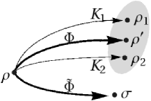
Figure 1: A quantum channel $\Phi$ represents a device preparing the ensemble of quantum states $\mathcal{E}=\{p_{i},\rho_{i}\}_{i=1}^{2}$. The average of this ensemble is denoted as $\rho^{\prime}=\Phi(\rho)=\sum_{i=1}^{2}K^{i}\rho K^{i\dagger}$. The complementary channel $\tilde{\Phi}$ transforms an initial state $\rho$ into the state $\sigma$ of the environment.

Independently of the interpretation of the Kraus operators $K^{i}$ the following theorem proved in [49] holds.

Theorem 4.

Let $\sum_{i=1}^{k}K^{i\dagger}K^{i}={\rm 1\rule{0.43057pt}{6.54443pt}\hskip 0.86108pt}$ be the identity decomposition and $\rho$ an arbitrary quantum state. Define the probability distribution $p_{i}=\operatorname*{Tr}K^{i}\rho K^{i\dagger}$ and a set of density matrices $\rho_{i}=\frac{K^{i}\rho K^{i\dagger}}{\operatorname*{Tr}K^{i}\rho K^{i\dagger}}$. The Holevo quantity $\chi(\{\rho_{i},p_{i}\})$ is bounded by the entropy of the correlation matrix, $\sigma=\sum_{i,j=1}^{k}\operatorname*{Tr}K^{i}\rho K^{j\dagger}|i\rangle\langle j|$:

$$\chi(\{\rho_{i},p_{i}\})=S\big{(}\sum_{i=1}^{k}p_{i}\rho_{i}\big{)}-\sum_{i=1}^{k}p_{i}S(\rho_{i})\leq S(\sigma)\leq H(P),$$ (87)

where $H(P)$ is the Shannon entropy of the probability distribution $P=\{p_{1},...,p_{k}\}$.

Proof.

The right hand side of the inequality: $S(\sigma)\leq H(P)$, is a consequence of the majorization theorem, see e.g. [15]. Since the probability vector $P$ forms a diagonal of a correlation matrix, we have $S(\sigma)\leq S({\rm diag}(\sigma))=H(P)$. The left hand side of the inequality (87) is proved due to the strong subadditivity of the von Neumann entropy [60]. The multipartite state $\omega_{123}$ is constructed in such a way that entropies of its partial traces are related to specific terms of (87).

The multipartite state $\omega_{123}$ is constructed by using an isometry $F|\phi\rangle=\sum_{i=1}^{k}|i\rangle\otimes|i\rangle\otimes K^{i}|\phi\rangle$. The state $\omega_{123}=F\rho F^{\dagger}$ is given explicitly by the formula

$$\omega_{123}=F\rho F^{\dagger}=\sum_{i,j=1}^{k}|i\rangle\langle j|\otimes|i\rangle\langle j|\otimes K^{i}\rho K^{j\dagger}.$$ (88)

States of the subsystems $\omega_{i}$ are given by partial traces over the remaining subsystems, for example, $\omega_{1}={\rm Tr}_{23}\omega_{123}$ and so on.

Let us introduce the following notation $A_{ij}=K^{i}\rho K^{j\dagger}$. In this notation the quantities from the Theorem 4 take the form $p_{i}=\operatorname*{Tr}A_{ii}$ and $\rho_{i}=A_{ii}/p_{i}$. Notice that

$$S(\omega_{12})=S(\sigma),$$ (89)

$$S(\omega_{3})=S\big{(}\sum_{i=1}^{k}p_{i}\rho_{i}\big{)}.$$ (90)

Moreover

$$-\sum_{i=1}^{k}p_{i}S(\rho_{i}) =\sum_{i=1}^{k}\operatorname*{Tr}A_{ii}\log A_{ii}-\sum_{i=1}^{k}\operatorname*{Tr}(A_{ii})\log\operatorname*{Tr}(A_{ii})$$

$$=S(\omega_{1})-S(\omega_{23}).$$ (91)

The strong subadditivity relation in the form which is used most frequently

$$S(\omega_{123})+S(\omega_{2})\leq S(\omega_{12})+S(\omega_{23})$$ (92)

does not lead to the desired form (87). However, due to the purification procedure and the fact that a partial trace of a pure state has the same entropy as the complementary partial trace, inequality (92) can be rewritten in an alternative form [21]:

$$S(\omega_{3})+S(\omega_{1})\leq S(\omega_{12})+S(\omega_{23}).$$ (93)

This inequality applied to the partial traces of the state (88) proves Theorem 4. ∎

For an ensemble of pure states $\rho_{i}=|\psi_{i}\rangle\langle\psi_{i}|$, the left hand side of (87) consists of the term $S(\sum_{i}p_{i}|\psi_{i}\rangle\langle\psi_{i}|)$ only. The correlation matrix $\sigma$ in the case of pure states is given by the Gram matrix. Due to the simple observation (55), the left inequality (87) is saturated in case of any ensemble $\mathcal{E}$ consisting of pure states only.

Using a different method an inequality analogous to Theorem 4 has been recently proved in [71] for the case of infinite dimension. It can be also found in [72] in context of quantum cryptography. The authors analyse there the security of a cryptographic key created by using so called ’private qubits’. In such a setup an inequality analogous to (87) appears as a bound on the information of the eavesdropper.

2.1 Other inequalities for the Holevo quantity

Methods similar to that used to prove Theorem 4 can be applied to prove other useful bounds.

Proposition 1.

Consider a POVM measurement characterized by operators $\sum_{i=1}^{k}K^{i\dagger}K^{i}={\rm 1\rule{0.43057pt}{6.54443pt}\hskip 0.86108pt}$ which define the outcome states, $\rho_{i}=\frac{K^{i}\rho K^{i\dagger}}{\operatorname*{Tr}K^{i}\rho K^{i\dagger}}$ and their probabilities, $p_{i}=\operatorname*{Tr}K^{i}\rho K^{i\dagger}$. The average entropy of the output states is smaller than entropy of the initial state,

$$\sum_{i=1}^{k}p_{i}S(\rho_{i})\leq S(\rho).$$ (94)

Proof.

Due to the fact that the transformation $F$ in Eq. (88) is an isometry, the three-partite state $\omega_{123}$ has the same nonzero spectrum as the initial state $\rho$. Hence $\omega_{123}$ and $\rho$ have the same entropy. Due to equality (91) and the Araki–Lieb inequality [76]:

$$S(\omega_{1})-S(\omega_{23})\leq S(\omega_{123}),$$ (95)

one completes the proof of Proposition 94. ∎

Note that concavity of entropy implies also another inequality $\sum_{i=1}^{k}p_{i}S(\rho_{i})\leq S(\rho^{\prime})=S(\sum_{i=1}^{k}p_{i}\rho_{i})$. Proposition 94 has been known before [77] as the quantum information gain.

Definition of the channel capacity (83) encourages one to consider bounds on the Holevo quantity for the concatenation of two quantum operations. Treating the probabilities $p_{i}$ and states $\rho_{i}$ as the outputs from the first channel one can replace maximization over $\mathcal{E}=\{\rho_{i},p_{i}\}_{i=1}^{k}$ in (83) by maximization over the initial state $\rho$ and the quantum operation $\Phi_{1}$. The strategy similar to that used in Theorem 4 allows us to prove the following relations.

Proposition 2.

Consider two quantum operations: $\Phi_{1}(\rho)=\sum_{i=1}^{k_{1}}K_{1}^{i}\rho K^{i\dagger}_{1}$ and $\Phi_{2}(\rho)=\sum_{i=1}^{k_{2}}K^{i}_{2}\rho K^{i\dagger}_{2}$. Define $p_{i}=\operatorname*{Tr}K^{i}_{1}\rho K_{1}^{i\dagger}$ and $\rho_{i}=\frac{K^{i}_{1}\rho K_{1}^{i\dagger}}{\operatorname*{Tr}K^{i}_{1}\rho K_{1}^{i\dagger}}$. The following inequality holds:

$$S\big{(}\Phi_{2}\circ\Phi_{1}(\rho)\big{)}-\sum_{i=1}^{k_{1}}p_{i}S\big{(}\Phi_{2}(\rho_{i})\big{)}\leq S(\Phi_{1}(\rho))-\sum_{i=1}^{k_{1}}p_{i}S(\rho_{i}).$$ (96)

Proof.

Let us consider the four–partite state:

$$\omega^{\prime}_{1234}=\sum_{n,l=1}^{k_{1}}\sum_{i,j=1}^{k_{2}}|i\rangle\langle j|\otimes|nn\rangle\langle ll|\otimes K^{i}_{2}K^{n}_{1}\rho K^{l\dagger}_{1}K^{j\dagger}_{2},$$ (97)

where $|nn\rangle\equiv|n\rangle\otimes|n\rangle$, and the strong subadditivity relation in the form

$$S(\omega^{\prime}_{124})+S(\omega^{\prime}_{4})\leq S(\omega^{\prime}_{14})+S(\omega^{\prime}_{24}).$$ (98)

Notice that

$$S(\omega^{\prime}_{4})=S(\Phi_{2}\circ\Phi_{1}(\rho)),$$

$$S(\omega^{\prime}_{3})-S(\omega^{\prime}_{24})=-\sum_{i}p_{i}S\big{(}\Phi_{2}(\rho_{i})\big{)},$$

$$S(\omega^{\prime}_{14})=S(\sum_{i,j=1}^{k_{2}}|i\rangle\langle j|\otimes K^{i}_{2}\Phi_{1}(\rho)K^{j\dagger}_{2})=S(\Phi_{1}(\rho)).$$

The third equality is due to the fact that an isometry, $F_{2}|\phi\rangle=\sum_{i=1}^{k_{2}}|i\rangle\otimes K^{i}_{2}|\phi\rangle$, does not change the nonzero part of spectrum. This property is also used to justify the following equation

$$S(\omega^{\prime}_{3})-S(\omega^{\prime}_{124})=-\sum_{i=1}^{k_{1}}p_{i}S(\rho_{i}).$$ (99)

Substituting these quantities to the strong subadditivity relation (98) we finish the proof. ∎

Inequality 96 is known [8] as the property that the Holevo quantity decreases under a quantum operation $\chi(p_{i},\rho_{i})\geq\chi(p_{i},\Phi(\rho_{i}))$.

Consider notation used in the proof of Proposition 96. Concavity of the entropy gives

$$\sum_{i=1}^{k_{1}}p_{i}S\Big{(}\Phi_{2}(\rho_{i})\Big{)}=\sum_{i=1}^{k_{1}}p_{i}S\Big{(}\sum_{j=1}^{k_{2}}q_{j}\rho_{ij}\Big{)}\geq\sum_{i=1}^{k_{1}}\sum_{j=1}^{k_{2}}p_{i}q_{j}S(\rho_{ij}).$$ (100)

where $\rho_{ij}=\frac{K^{j}_{2}K^{i}_{1}\rho K^{i\dagger}_{1}K^{j\dagger}_{2}}{\operatorname*{Tr}K^{j}_{2}K^{i}_{1}\rho K^{i\dagger}_{1}K^{j\dagger}_{2}}$ and probabilities $p_{i}q_{j}=\operatorname*{Tr}K^{j}_{2}K^{i}_{1}\rho K^{i\dagger}_{1}K^{j\dagger}_{2}$. Using Theorem 4 and concavity of entropy (100) one proves:

Proposition 3.

Consider two quantum operations: $\Phi_{1}(\rho)=\sum_{i=1}^{k_{1}}K^{i}_{1}\rho K^{i\dagger}_{1}$ and $\Phi_{2}(\rho)=\sum_{i=1}^{k_{2}}K^{i}_{2}\rho K^{i\dagger}_{2}$. Define $p_{i}=\operatorname*{Tr}K^{i}_{1}\rho K_{1}^{i\dagger}$ and $\rho_{i}=\frac{K^{i}_{1}\rho K_{1}^{i\dagger}}{\operatorname*{Tr}K^{i}_{1}\rho K_{1}^{i\dagger}}$. The following inequality holds:

$$S\Big{(}\Phi_{2}\circ\Phi_{1}(\rho)\Big{)}-\sum_{i=1}^{k_{1}}p_{i}S\Big{(}\Phi_{2}(\rho_{i})\Big{)}\leq S(\sigma_{II}),$$ (101)

where the output of the complementary channel to $\Phi_{2}\otimes\Phi_{1}$ is denoted as $\sigma_{II}=\widetilde{\Phi_{2}\circ\Phi_{1}}(\rho)$.

2.1.1 Some consequences

This section provides three applications of theorems proved in Sections 2 and 2.1. One of them concerns the coherent information. This quantity is defined for a given quantum operation $\Phi$ and an initial state $\rho$ as follows [73]

$$I_{coh}(\Phi,\rho)=S\big{(}\Phi(\rho)\big{)}-S\big{(}\tilde{\Phi}(\rho)\big{)},$$ (102)

where $\tilde{\Phi}(\rho)$ is the output state of the channel complementary to $\Phi$. To some extent, coherent information in quantum information theory plays a similar role to mutual information in classical information theory. It is known [8] that $I_{coh}(\Phi,\rho)\leq S(\rho)$. That is a relation similar to (74). Moreover, it has been shown that only if $I_{coh}(\Phi,\rho)=S(\rho)$ the process $\Phi$ can be perfectly reversed. In this case the perfect quantum error correction is possible [73]. The coherent information is also used to define the quantum capacity of a quantum channel [74]

$$C_{Q}(\Phi)=\max_{\rho}I_{coh}(\Phi,\rho).$$ (103)

The definition of the coherent information (102) can be formulated alternatively [73] by means of an extended quantum operation $\Phi\otimes\operatorname{id}$ acting on a purification $|\psi\rangle\in\mathcal{H}_{2}\otimes\mathcal{H}_{3}$ of an initial state, $\rho={\rm Tr}_{3}|\psi\rangle\langle\psi|$. This fact is justified as follows. The purification of $\rho$ determines as well the purification $\Omega_{123}\in\mathcal{H}_{1}\otimes\mathcal{H}_{2}\otimes\mathcal{H}_{3}$ of the state $\omega\in\mathcal{H}_{1}\otimes\mathcal{H}_{2}$ in (29),

$$\Omega_{123}=U_{12}\otimes\operatorname{id}_{3}\Big{(}|1\rangle\langle 1|_{1}\otimes|\psi\rangle\langle\psi|_{23}\Big{)}U_{12}^{\dagger}\otimes\operatorname{id}_{3}.$$ (104)

The partial trace over the environment (subspace $\mathcal{H}_{1}$) reads

$$\Omega_{23}=[\Phi\otimes\operatorname{id}]\left(|\psi\rangle\langle\psi|\right).$$ (105)

It has the same entropy as the partial trace over the second and third subspace, $\Omega_{1}=\sigma,$ which is a state of environment after evolution,

$$S(\sigma)=S([\Phi\otimes\operatorname{id}]\left(|\psi\rangle\langle\psi|\right)),$$ (106)

and $S(\sigma)=S(\tilde{\Phi}(\rho))$.

Coherent information (102) can be written as

$$I_{coh}(\Phi,\rho)=S({\rm Tr}_{3}\Omega_{23})-S(\Omega_{23}).$$ (107)

The classical counterpart of the coherent information can be defined by using the Shannon entropy instead of the von Neumann entropy and probability vectors instead of density matrices in Eq. (107). The classical coherent information is always negative, since the entropy of a joint probability distribution cannot be smaller than its marginal distribution.

Inequalities proved in Theorem 4 and Proposition 94 together provide the following bound on the coherent information,

$$I_{coh}(\Phi,\rho)\leq\sum_{i=1}^{k}p_{i}S(\rho_{i})\leq S(\rho),$$ (108)

where $p_{i}=\operatorname*{Tr}K^{i}\rho K^{i\dagger}$ and $\rho_{i}=K^{i}\rho K^{i\dagger}/p_{i}$ are defined by Kraus representations of the channel, $\Phi(\rho)=\sum_{i=1}^{k}K^{i}\rho K^{i\dagger}$. The equality between coherent information and the entropy of initial state $S(\rho)$ guarantees that $\Phi$ is reversible. Inequality (108) implies a similar, weaker statement: only if the following equality holds $\sum_{i=1}^{k}p_{i}S(\rho_{i})=S(\rho)$, the quantum operation $\Phi$ can be reversed.

Another consequence of inequalities proved in Section 2.1 concerns the so called degradable channels. These channels are considered in quantum information theory in the context of their capacity [42]. A channel $\Phi_{deg}$ is called degradable if there exists a channel $\Psi$ such that $\Psi\circ\Phi_{deg}=\tilde{\Phi}_{deg}$. Substituting the degradable channel $\Phi_{1}=\Phi_{deg}$ and the additional channel $\Phi_{2}=\Psi$ to inequality in Proposition 96 one obtains a lower bound for the average entropy of $\Psi(\rho_{i})$, where $\rho_{i}$ are output states from the channel $\Phi_{deg}$,

$$0\leq\sum_{i=1}^{k}p_{i}S(\rho_{i})-I_{coh}(\Phi_{\deg},\rho)\leq\sum_{i=1}^{k}p_{i}S\big{(}\Psi(\rho_{i})\big{)},$$ (109)

where $I_{coh}(\Phi,\rho)=S\big{(}\Phi_{deg}(\rho)\big{)}-S\big{(}\tilde{\Phi}_{deg}(\rho)\big{)}$. The left inequality is due to inequality (108). Therefore Proposition 96 provides some characterization of the channel $\Psi$ which is associated with a degradable channel.

The third application of propositions from Section 2.1 is given as follows. The Jamiołkowski isomorphism [34] gives a representation of a quantum map $\Phi$ which acts on $N$ dimensional system by a density matrix on the extended space of size $N^{2}$. This state can be written as:

$$\sigma_{\Phi}=[\operatorname{id}\otimes\Phi]\big{(}\left|\phi^{+}\right\rangle\left\langle\phi^{+}\right|\big{)},$$ (110)

where $\left|\phi^{+}\right\rangle=\frac{1}{\sqrt{N}}\sum_{i=1}^{N}\left|i\right\rangle\otimes\left|i\right\rangle$ is the maximally entangled state. A rescaled state $D_{\Phi}=N\sigma_{\Phi}$ is called the dynamical matrix. In the special case, if the initial state is maximally mixed, $\rho=\frac{1}{N}{\rm 1\rule{0.43057pt}{6.54443pt}\hskip 0.86108pt}$, the entropy of the correlation matrix $\sigma$ written in (106) is equal to the entropy of the dynamical matrix.

A quantum map $\Phi$ can by defined using its Kraus representation (30). Since the Kraus representation is not unique [15], one can associate many different correlation matrices with a given quantum operation $\Phi$ depending on both, the initial state and the set of Kraus operators. However the entropy of the dynamical matrix $D_{\Phi}$ is invariant under different decompositions. This entropy characterizes the quantum operation and is called the entropy of a map [49], denoted by $S^{\operatorname*{map}}(\Phi)$ as defined in Eq. (45).

Due to Theorem 4 the entropy of a map has the following interpretation. It determines an upper bound on the Holevo quantity (76) for a POVM measurement defined by the Kraus operators of $\Phi$ if the initial state is maximally mixed $\rho=\rho_{*}=\frac{1}{N}{\rm 1\rule{0.43057pt}{6.54443pt}\hskip 0.86108pt}$. Moreover, the entropy of a map is an upper bound for the Holevo quantity for POVM given by any set of Kraus operators $\{K^{i\dagger}K^{i}\}$ which realize the same quantum operation $\Phi$,

$$\max_{\{K^{i}\}}\quad\chi\Big{(}\{p_{i}=\operatorname*{Tr}K^{i}\rho_{*}K^{i\dagger},\ \ \rho_{i}=\frac{K^{i}\rho_{*}K^{i\dagger}}{\operatorname*{Tr}K^{i}\rho_{*}K^{i\dagger}}\}\Big{)}\leq S(\Phi),$$ (111)

where $\rho^{\prime}=\Phi(\rho)=\sum_{i=1}^{k}K^{i}\rho K^{i\dagger}$.

Proposition 3 provides also an alternative lower bound for the entropy of composition of two quantum maps given by Theorem 3 in [46]. The inequality for the entropy of composition of two maps can be now stated as

$$0\leq{\rm MAX}\Big{\{}S(\Phi_{2}\circ\Phi_{1}(\rho_{*}))-\sum_{i=1}^{k}p_{i}S(\Phi_{2}(\rho_{i})),\ S(\Phi_{1})+\Delta\Big{\}}\leq S(\Phi_{2}\circ\Phi_{1}),$$ (112)

where $\Delta=S\big{(}\Phi_{2}\circ\Phi_{1}(\rho_{*})\big{)}-S\big{(}\Phi_{1}(\rho_{*})\big{)}$ and $\Phi(\rho)=\sum_{i=1}^{k}p_{i}\rho_{i}$. The lower bound proved in our earlier paper [46] could be smaller than $0$. The improved bound is always greater than $0$ due to concavity of entropy.

2.2 Discussion on the Lindblad inequality

Lindblad [75] proved an inequality which relates the von Neumann entropy of a state $\rho$, its image $\rho^{\prime}=\Phi(\rho)=\sum_{i=1}^{k}p_{i}\rho_{i}$ and the entropy of the correlation matrix $\sigma$ equal to the output state of the complementary channel $\sigma=\tilde{\Phi}(\rho)$,

$$|S(\rho^{\prime})-S(\rho)|\leq S(\sigma)\leq S(\rho^{\prime})+S(\rho).$$ (113)

Another two Lindblad inequalities are obtained by permuting the states $\rho,\rho^{\prime}$ and $\sigma$ in this formula. The proof of Lindblad proceeds in a similar way to the proof of Theorem 4. It involves a bi–partite auxiliary state $\omega^{\prime\prime}=\sum_{i,j=1}^{k}|i\rangle\langle j|\otimes K_{i}\rho K_{j}^{\dagger}$, where the identity $S(\rho)=S(\omega^{\prime\prime})$ is due to an isometry similar to $F$ in (88). The Araki–Lieb inequality [76], $|S(\rho_{1})-S(\rho_{2})|\leq S(\rho_{12})$ applied to $\omega^{\prime\prime}$ proves the left hand side inequality of (113), while the subadditivity relation $S(\rho_{12})\leq S(\rho_{1})+S(\rho_{2})$ applied to $\omega^{\prime\prime}$ proves the right hand side inequality of (113).

Inequalities from Theorem 4 and Proposition 94

$$S(\rho^{\prime})-\sum_{i=1}^{k}p_{i}S(\rho_{i})\leq S(\sigma),$$ (114)

$$\sum_{i=1}^{k}p_{i}S(\rho_{i})\leq S(\rho)$$ (115)

use a three–partite auxiliary state $\omega=\sum_{i,j=1}^{k}|ii\rangle\langle jj|\otimes K_{i}\rho K_{j}^{\dagger}$. As in the case of the Lindblad inequality (113), the identity $S(\rho)=S(\omega)$ holds due to isometry. The strong subadditivity relation applied to $\omega$ proves inequality (114), while the Araki–Lieb inequality applied for $\omega$ proves inequality (115). Notice that an extension of the auxiliary state and application of the strong subadditivity relation allows one to use the average entropy to new inequalities for interesting quantities: the entropy of the initial state, the entropy of the output state of a quantum channel $\rho^{\prime}=\Phi(\rho)$ and the entropy of the output state of the complementary channel $\tilde{\Phi}(\rho)$.

In the case $S(\rho^{\prime})\geq S(\rho)$ (e.g. for any bistochastic operations) the result (114) gives a better lower constraints for $S(\sigma)$ than the Lindblad bound (113). In this case

$$S(\rho^{\prime})-S(\rho)\leq S(\rho^{\prime})-\sum_{i=1}^{k}p_{i}S(\rho_{i})\leq S(\sigma),$$ (116)

due to Prop. 94. However, if $S(\rho^{\prime})\leq S(\rho)$ the result of Lindblad can be more precise depending on the values of $S(\rho)$, $S(\rho^{\prime})$ and the average entropy $\sum_{i=1}^{k}p_{i}S(\rho_{i})$. In consequence, due to Lindblad inequality (113) and the inequality (111) one obtains another lower bound for the entropy of a map:

$${\rm MAX}\Big{\{}\log(N)-S(\Phi(\rho_{*})),\ \ \ \max_{\{K^{i}\}}\ \chi\Big{(}p_{i}=\operatorname*{Tr}K^{i}\rho_{*}K^{i\dagger},\ \ \rho_{i}=\frac{K^{i}\rho_{*}K^{i\dagger}}{\operatorname*{Tr}K^{i}\rho_{*}K^{i\dagger}}\Big{)}\Big{\}}\leq S^{\operatorname*{map}}(\Phi),$$ (117)

where $\rho^{\prime}=\Phi(\rho)=\sum_{i=1}^{k}K^{i}\rho K^{i\dagger}=\sum_{i=1}^{k}p_{i}\rho_{i}$.

2.3 Inequalities for other entropies

Inequality (87) uses the strong subadditivity relation in the form (93) which is a specific feature of the von Neumann entropy. Relation (93) can be equivalently formulated in terms of relative von Neumann entropies.

The relative von Neumann entropy $D(\rho_{1},\rho_{2})$ is defined as follows

$$D(\rho_{1},\rho_{2})=\operatorname*{Tr}\rho_{1}\big{[}\log{\rho_{1}}-\log(\rho_{2})\big{]}$$ (118)

and is finite for $\rho_{2}\in{\rm supp}(\rho_{1})$, otherwise it becomes infinite.

Monotonicity of relative entropy states that for any three–partite quantum state $\omega_{123}$ and its partial traces the following inequality holds:

$$D(\omega_{23},\omega_{2}\otimes\omega_{3})\leq D(\omega_{123},\omega_{12}\otimes\omega_{3}).$$ (119)

It is an important and nontrivial property of the von Neumann entropy [60], [78]. Monotonicity of the von Neumann entropy (119) rewritten using the definition (118) leads to the strong subadditivity relation:

$$S(\omega_{123})+S(\omega_{3})\leq S(\omega_{13})+S(\omega_{23}).$$ (120)

Complementary partial traces of any multipartite pure state have the same entropy. This fact can be applied to purifications of $\omega_{123}$. Therefore, relation (120) is equivalent to (93) which can be applied to the specific three–partite state (88)

$$\omega_{123}=\sum_{i,j=1}^{k}|i\rangle\langle j|\otimes|i\rangle\langle j|\otimes K_{i}\rho K_{j}^{\dagger}$$ (121)

and used to prove the upper bound on the Holevo quantity in terms of a correlation matrix $\chi\leq S(\sigma)$. Hence, inequality (87) is a consequence of the monotonicity of the relative von Neumann entropy.

Monotonicity of entropy holds also for some generalized entropies e.g. Tsallis entropies of order $0\leq\alpha<1$ [79] or Rényi entropies of order $0\leq q\leq 2$ [80]. Direct generalization of $\chi\leq S(\sigma)$ is not so easy, since the key step in the proof was the strong subadditivity form (93). In case of generalized entropies such a form cannot be obtained from the monotonicity of relative entropy.

The Holevo quantity can be expressed by the relative entropy. Consider the state (121) and the notation: $K^{i}\rho K^{i\dagger}=p_{i}\rho_{i}$, and $\sum_{i=1}^{k}p_{i}\rho_{i}=\rho^{\prime}$. The relative entropy reads:

$$D(\omega_{23},\omega_{2}\otimes\omega_{3})=$$ (122)

$$= \operatorname*{Tr}\omega_{23}\log{\omega_{23}}-\operatorname*{Tr}\omega_{23}\log{\omega_{2}}-\operatorname*{Tr}\omega_{23}\log\omega_{3}$$ (123)

$$= \sum_{i=1}^{k}\operatorname*{Tr}p_{i}\rho_{i}\log{p_{i}\rho_{i}}-\sum_{i=1}^{k}p_{i}\log{p_{i}}-\operatorname*{Tr}\rho^{\prime}\log{\rho^{\prime}}$$ (124)

$$= \sum_{i=1}^{k}p_{i}\operatorname*{Tr}\rho_{i}\log{\rho_{i}}-\operatorname*{Tr}\rho^{\prime}\log{\rho^{\prime}}$$ (125)

$$= S(\rho^{\prime})-\sum_{i=1}^{k}p_{i}S(\rho_{i})=\sum_{i=1}^{k}p_{i}D(\rho_{i},\rho^{\prime})=\chi.$$ (126)

The equality between the Holevo quantity and relative entropy holds also for the Tsallis entropies of any order $q$

$$T_{\alpha}(\rho)=\frac{1}{1-\alpha}\Big{[}1-\operatorname*{Tr}\rho^{\alpha}\Big{]},$$ (127)

where the relative Tsallis entropy $D^{T}_{\alpha}$ of order ${\alpha}$ is defined as [79]

$$D^{T}_{\alpha}(\rho_{1},\rho_{2})=\frac{1}{{\alpha}-1}\Big{[}1-\operatorname*{Tr}\rho_{1}^{\alpha}\rho_{2}^{1-{\alpha}}\Big{]}.$$ (128)

It is now possible to compute the Tsallis–like generalized relative entropy $D^{T}_{\alpha}$ between a bipartite state $\omega_{23}$ and the product of its partial traces which leads to the generalized Holevo quantity $\chi^{T}_{\alpha}$. If one considers the state (121)

$$D^{T}_{\alpha}(\omega_{23},\omega_{2}\otimes\omega_{3}) = \frac{1}{{\alpha}-1}\Big{[}1-\operatorname*{Tr}\omega_{23}^{\alpha}(\omega_{2}\otimes\omega_{3})^{1-{\alpha}}\Big{]}$$ (129)

$$= \frac{1}{{\alpha}-1}\Big{[}1-\sum_{i=1}^{k}\operatorname*{Tr}(p_{i}\rho_{i})^{\alpha}p_{i}^{1-{\alpha}}\rho^{\prime 1-{\alpha}}\Big{]}$$ (130)

$$= \sum_{i=1}^{k}p_{i}\frac{1}{{\alpha}-1}(1-\operatorname*{Tr}\rho_{i}^{\alpha}\rho^{\prime 1-{\alpha}})$$ (131)

$$= \sum_{i=1}^{k}p_{i}D^{T}_{\alpha}(\rho_{i},\rho^{\prime})\equiv\chi^{T}_{\alpha}.$$ (132)

In a similar way we can work with the Rényi entropy $S_{q}^{R}(\rho)=\frac{1}{1-\alpha}\log[\operatorname*{Tr}\rho^{\alpha}]$. The corresponding relative Rényi entropy reads [81]

$$D^{R}_{q}(\rho_{1},\rho_{2})=\frac{1}{q-1}\log\operatorname*{Tr}[\rho_{1}^{q}\rho_{2}^{1-q}]$$ (133)

and the Rényi–Holevo quantity is given by

$$\chi^{R}_{q}=\frac{1}{q-1}\log\operatorname*{Tr}(\sum_{i}p_{i}\rho_{i}^{q})^{1/q}.$$ (134)

Equality between the generalized Rényi–Holevo quantity (134) and the Rényi relative entropy (133) holds if relative entropy concerns partial traces of (121) and the state $\rho^{\prime\prime}=(\sum_{i}p_{i}\rho_{i}^{q})^{1/q}$ as follows

$$\chi^{R}_{q}=D^{R}_{q}(\omega_{23},\omega_{2}\otimes\rho^{\prime\prime}).$$ (135)

The Holevo quantity (135) is smaller than $D^{R}_{q}(\omega_{23},\omega_{2}\otimes\omega_{3})$ [81].

The monotonicity of relative entropy for three considered types of generalized entropies: von Neumann entropy, Tsallis entropy of order $0\leq\alpha<1$ and Rényi entropy of order $0\leq q\leq 2$ gives

$$\chi\leq D(\omega_{123},\sigma\otimes\rho^{\prime}),$$ (136)

$$\chi^{T}_{\alpha}\leq D^{T}_{\alpha}(\omega_{123},\sigma\otimes\rho^{\prime}),$$ (137)

$$\chi^{R}_{q}\leq D^{R}_{q}(\omega_{123},\sigma\otimes\rho^{\prime}).$$ (138)

These relations state that the Holevo quantity is bounded by the relative entropy between the joint state of the quantum system and its environment and the states of these subsystems taken separately.

In case of von Neumann entropy, inequality (136) can be written explicitly as

$$\chi\leq S(\sigma)+S(\rho^{\prime})-S(\rho).$$ (139)

Notice that $\rho$ is an initial state and $S(\rho)=S(\omega_{123})$ due to isometry transformation, $F:\rho\rightarrow\omega_{123}$. Relation (139) joints entropies of the initial state, the final state, the state of the environment and the Holevo quantity in a single formula. Inequality (139) which can be rewritten as

$$S(\rho)\leq S(\sigma)+\sum_{i=1}^{k}p_{i}S(\rho_{i})$$ (140)

gives a finer bound than that provided by the Lindblad inequality: $S(\rho)\leq S(\sigma)+S(\rho^{\prime})$. Inequality (139) can be written as $\chi\leq S(\sigma)+Y$, where $|Y|=|S(\rho^{\prime})-S(\rho)|\leq S(\sigma)$, due to one of the Lindblad inequalities. In some cases this inequality confines the relation (87).

2.4 Searching for the optimal bound

The state $\sigma$ can be defined for a triple consisting of a probability distribution, set of $k$ density matrices of size $N$ and a set of $k$ unitary matrices, $\{p_{i},\rho_{i},U_{i}\}_{i=1}^{k}$. Every triple $(p_{i},\rho_{i},U_{i})$ defines uniquely the pure state $|\psi_{i}\rangle$ which is the purification of state $\rho_{i}$ as follows

$$|\psi_{i}\rangle=\sum_{r=1}^{N}(U_{i}\otimes\sqrt{\rho_{i}}V_{i})|e_{r}\rangle\otimes|e_{r}\rangle$$ (141)

as shown in (49). The Holevo quantity depends only on $\mathcal{E}=\{p_{i},\rho_{i}\}_{i=1}^{k}$. Therefore, Theorem 4 can be reformulated as follows:

Theorem 5.

For any ensemble $\{p_{i},\rho_{i},U_{i}\}_{i=1}^{k}$ the Holevo quantity is bounded by the entropy of the correlation matrix $\sigma$ minimized over all unitary matrices $U_{i}$

$$\chi(\{p_{i},\rho_{i}\})=S(\sum_{i=1}^{k}p_{i}\rho_{i})-\sum_{i=1}^{k}p_{i}S(\rho_{i})\leq\min_{\{U_{i}\}}S(\sigma)=\min_{\{U_{i}\}}S(\sum_{i=1}^{k}p_{i}|\psi_{i}\rangle\langle\psi_{i}|),$$ (142)

where $|\psi_{i}\rangle=\sum_{r=1}^{N}(U_{i}\otimes\sqrt{\rho_{i}}V_{i})|e_{r}\rangle\otimes|e_{r}\rangle$ and $\sigma_{ij}=\sqrt{p_{i}p_{j}}\operatorname*{Tr}\sqrt{\rho_{i}}\sqrt{\rho_{j}}U_{j}^{\dagger}U_{i}$.

The last equality of (142) holds since the correlation matrix $\sigma$ can be represented as the Gram matrix of purifications of $\rho_{i}$. It is known that for any Gram matrix equality (55) holds.

Finding minimization of $S(\sigma)$ over unitaries is not an easy problem in general. In the following chapter the problem will be solved for the ensemble of $k=2$ states, and the solution is written in terms of square root of the fidelity between both states. A conjecture that the matrix of the square roots of fidelities also bounds the Holevo quantity for ensembles of $k=3$ states will be formulated and some weaker bounds will be proved in the next section.

2.4.1 Optimal bound for two matrices

The tightest upper bound on the Holevo quantity occurring in Theorem 5 is obtained by taking minimum of $S(\sigma)$ over the set of unitaries. This is equivalent to the POVM which minimizes the correlation matrix among all POVM which give the same output states. For two output states $\rho_{1}$ and $\rho_{2}$ occurring with probabilities $(\lambda,1-\lambda)$ the correlation matrix is given by

$$\sigma=\begin{pmatrix}\lambda&\sqrt{\lambda(1-\lambda)}\operatorname*{Tr}\sqrt{\rho_{1}}\sqrt{\rho_{2}}U_{2}^{\dagger}U_{1}\\ \sqrt{\lambda(1-\lambda)}\operatorname*{Tr}\sqrt{\rho_{2}}\sqrt{\rho_{1}}U_{1}^{\dagger}U_{2}&1-\lambda\end{pmatrix}.$$ (143)

Its entropy is the lowest, if the absolute values of the off–diagonal elements are the largest. As has been shown in Eq. (67) the expression $\operatorname*{Tr}\sqrt{\rho_{1}}\sqrt{\rho_{2}}U_{2}^{\dagger}U_{1}$ attains its maximum over unitary matrices at the value

$$\sqrt{F_{12}}=\operatorname*{Tr}{\sqrt{\sqrt{\rho_{1}}\rho_{2}\sqrt{\rho_{1}}}},$$ (144)

where for brevity we use $F_{12}$ instead of $F(\rho_{1},\rho_{2})$. This quantity is equal to the square root fidelity (62). Therefore the correlation matrix of the smallest entropy can be rewritten in terms of the square root fidelity,

$$\sigma_{min}=\begin{pmatrix}\lambda&\sqrt{\lambda(1-\lambda)}\sqrt{F_{12}}\\ \sqrt{\lambda(1-\lambda)}\sqrt{F_{12}}&1-\lambda\end{pmatrix}.$$ (145)

2.5 Jensen Shannon Divergence

Minimal entropy of the correlation matrix characterizing an ensemble of two density matrices is related to the distance between them in the set of density matrices. If the probability distribution in (145) is uniform, $\lambda=1/2$, the square root of the von Neumann entropy of $\sigma_{min}$ forms a metric [53]. It is called the entropic distance $D_{E}(\rho_{1},\rho_{2})$

$$D_{E}(\rho_{1},\rho_{2})=\sqrt{S(\sigma_{min})},\qquad\sigma_{min}=\frac{1}{2}\begin{bmatrix}1&\sqrt{F(\rho_{1},\rho_{2})}\\ \sqrt{F(\rho_{1},\rho_{2})}&1\end{bmatrix}.$$ (146)

Inequality (142) provides the relation between this metric and another one defined by means of the Jensen–Shannon Divergence. The Jensen–Shannon Divergence $JSD(\{\alpha_{\nu}P_{\nu}\})$ has been initially defined [69], [82] as the divergence of classical probability distributions $P_{\nu}$ occurring with probabilities $\alpha_{\nu}$

$$JSD(\{\alpha_{\nu}P_{\nu}\})=H\Big{(}\sum_{\nu}\alpha_{\nu}P_{\nu}\Big{)}-\sum_{\nu}\alpha_{\nu}H(P_{\nu})=\sum_{\nu}\alpha_{\nu}H(P_{\nu}||\bar{P})$$ (147)

where $H(P)$ denotes the Shannon entropy of the probability distribution $P$, $H(P_{\nu}||\bar{P})$ is the relative entropy between $P_{\nu}$ and $\bar{P}$, while the average probability distribution reads $\bar{P}=\sum_{\nu}\alpha_{\nu}P_{\nu}$.

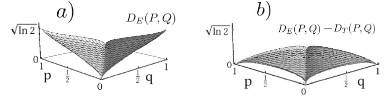
Figure 2: $a)$ The entropic distance $D_{E}$ (146) for two $2$–point probability distributions $P=(p,1-p)$ and $Q=(q,1-q)$. $b)$ The difference between the entropic distance $D_{E}$ and the transmission distance $D_{T}$ (149).

The square root of the Jensen-Shannon divergence between two probability distributions $P$ and $Q$,

$$JSD(P||Q)=\frac{1}{2}H(P||M)+\frac{1}{2}H(P||M),$$ (148)

where $M=\frac{1}{2}(P+Q)$, forms a metric in the set of classical probability distributions [82], [83] called the transmission distance $D_{T}(P,Q)$,

$$D_{T}(P,Q)=\sqrt{JSD(P||Q)}.$$ (149)

A probability distribution can be considered as a diagonal density matrix. Therefore, Eq. (142) in Theorem 5 demonstrates a relation between functions of two distances in the set of diagonal density matrices. Fig. 2 and Fig. 3 shows the comparison between these two distances for exemplary probability distributions.

A quantum counterpart of the Jensen–Shannon divergence, in fact coinciding with the Holevo quantity, was also considered [69], [82]. Inequality (142) provides thus an upper bound on the quantum Jensen–Shannon divergence.

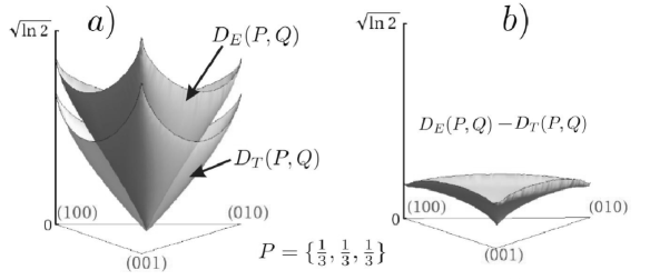
Figure 3: $a)$ The entropic distance $D_{E}$ (146) and the transmission distance $D_{T}$ (149) for two probability distributions, $P=(\frac{1}{3},\frac{1}{3},\frac{1}{3})$ and $Q=(q_{1},q_{2},q_{3})$ which is arbitrary distribution of dimension $3$ represented by a point in the simplex – the base of the figure. $b)$ The difference between the entropic distance $D_{E}$ and the transition distance $D_{T}$ for the same distributions $P$ and $Q$.

3 Conjecture on three–fidelity matrix

The minimization problem for the entropy of the correlation matrix (143) has been solved for an ensemble consisting of $k=2$ quantum states. In this case the solution is given by the square root fidelity matrix. In the case of $k=3$ states in the ensemble the optimization over the set of three unitary matrices is more difficult. Our numerical tests support the following conjecture, which is a generalization of the bound found for the case of $k=2$.

Conjecture 1.

For an ensemble of $k=3$ quantum states, $\{p_{i},\rho_{i}\}_{i=1}^{3}$ the entropy of the square root fidelity matrix $G_{ij}=\sqrt{p_{i}p_{j}}\sqrt{F(\rho_{i},\rho_{j})}$ gives the upper bound on the Holevo quantity,

$$\chi(\{p_{i},\rho_{i}\})\leq S\left(\begin{bmatrix}p_{1}&\sqrt{p_{1}p_{2}}\sqrt{F_{12}}&\sqrt{p_{1}p_{3}}\sqrt{F_{13}}\\ \sqrt{p_{2}p_{1}}\sqrt{F_{21}}&p_{2}&\sqrt{p_{2}p_{3}}\sqrt{F_{23}}\\ \sqrt{p_{3}p_{1}}\sqrt{F_{31}}&\sqrt{p_{3}p_{2}}\sqrt{F_{32}}&p_{3}\end{bmatrix}\right),$$ (150)

where fidelity between two quantum states reads $F_{ij}=F(\rho_{i},\rho_{j})=\big{(}{\rm Tr}\sqrt{\sqrt{\rho_{i}}\rho_{j}\sqrt{\rho_{i}}}\big{)}^{2}$.

It has been shown [84], [52] that the matrix $G$ containing square root fidelities is positively semi–defined for $k=3$. However, the square root fidelity matrix is in general not positive for $k>3$. Numerical tests provide several counterexamples for positivity of $G$ for $k>3$, even in case of an ensemble of pure states. Note that the matrix $G$ is not a special case of the correlation matrix $\sigma$, which is positive by construction.

Theorem 4 implies that Conjecture 1 holds for ensembles containing three pure states. Inequality (87) is in this case saturated as discussed in section 2. Square root fidelity matrix $G$ is obtained from the Gram matrix of given pure states by taking modulus of its matrix entries. Taking modulus of entries of a positive $3\times 3$ matrix does not change neither the trace nor the determinant of the matrix. Only the second symmetric polynomial of the eigenvalues is growing. Since the entropy is a monotonic increasing function of the second symmetric polynomial [67], the entropy of the square root fidelity matrix $G$ is larger than the entropy of the Gram matrix and therefore it is also larger than the Holevo quantity.

3.1 A strategy of searching for a proof of the conjecture

The proof of Theorem 4 consist of two steps. In the first step one has to find suitable multipartite state. In the second step the strong subadditivity relation of entropy has to be applied for the constructed multipartite state. The same strategy will be used searching for the proof of Conjecture 1 or for proving other weaker inequalities.

For the purpose of obtaining the Holevo quantity from suitable terms of the strong subadditivity relation, the multipartite state $\omega$ should have a few features:

• it is a block matrix which is positive,

• blocks on the diagonal should contain states $\rho_{i}$ multiplied by probabilities $p_{i}$,

• traces of off-diagonal blocks should give square root fidelities, or some smaller numbers if one aims to obtain a weaker bound.

The following matrix satisfies above conditions,

$$X=\begin{bmatrix}p_{1}\rho_{1}&0&0\mid&0&*&0\mid&0&0&*\\ 0&0&0\mid&0&0&0\mid&0&0&0\\ \underline{0}&\underline{0}&\underline{0}\mid&\underline{0}&\underline{0}&\underline{0}\mid&\underline{0}&\underline{0}&\underline{0}\\ 0&0&0\mid&0&0&0\mid&0&0&0\\ *&0&0\mid&0&p_{2}\rho_{2}&0\mid&0&0&*\\ \underline{0}&\underline{0}&\underline{0}\mid&\underline{0}&\underline{0}&\underline{0}\mid&\underline{0}&\underline{0}&\underline{0}\\ 0&0&0\mid&0&0&0\mid&0&0&0\\ 0&0&0\mid&0&0&0\mid&0&0&0\\ *&0&0\mid&0&*&0\mid&0&0&p_{3}\rho_{3}\\ \end{bmatrix},$$ (151)

where in place of $*$ one can put any matrix, provided the matrix $X$ remains positive. If in place of $*$ one substitutes zeros, the strong subadditivity relation implies the known formula that $\chi(\{p_{i},\rho_{i}\})\leq S(\{p_{i}\})$. Examples presented in the next section use described strategy to prove some entropic inequalities for the Holevo quantity.

The main problem is to find a suitable positive block matrix. In order to check positivity the Schur complement method [85] is very useful.

Lemma 1 (Schur).

Assume that $A$ is invertible and positive matrix, then

$$X=\begin{bmatrix}A&B\\ B^{\dagger}&C\end{bmatrix}$$ (152)

is positive if and only if $\mathsf{S}=C-B^{\dagger}A^{-1}B$ is positive semi–definite:

$$A>0\ =>\ (X>0\ <=>\ \mathsf{S}\geq 0).$$ (153)

The matrix $\mathsf{S}$ is called the Schur complement.

3.1.1 Three density matrices of an arbitrary dimension

The strategy mentioned in the previous section will be used to prove the following

Proposition 4.

For a three states ensemble $\{p_{i},\rho_{i}\}_{i=1,2,3}$ the following bound for the Holevo quantity $\chi$ holds

$$\chi(p_{i},\rho_{i})\leq S\left(\begin{bmatrix}p_{1}&\sqrt{p_{1}p_{2}}\sqrt{F_{12}}/b&\sqrt{p_{1}p_{3}}\sqrt{F_{13}}/b\\ \sqrt{p_{2}p_{1}}\sqrt{F_{21}}/b&p_{2}&\sqrt{p_{2}p_{3}}\sqrt{F_{23}}/b\\ \sqrt{p_{3}p_{2}}\sqrt{F_{31}}/b&\sqrt{p_{3}p_{2}}\sqrt{F_{32}}/b&p_{3}\end{bmatrix}\right),$$ (154)

where $b\geq 2$.

Proof.

It will be assumed that considered density matrices $\{\rho_{i}\}_{i=1}^{3}$ are invertible. After [106] the square root of the product of two density matrices $\sqrt{\rho\sigma}$ will be defined as follows:

$$\sqrt{\rho\sigma}\equiv\rho^{1/2}\sqrt{\rho^{1/2}\sigma\rho^{1/2}}\rho^{-1/2}=\sigma^{-1/2}\sqrt{\sigma^{1/2}\rho\sigma^{1/2}}\sigma^{1/2}.$$ (155)

In this notation the fidelity between two states $\rho_{i}$ and $\rho_{j}$ can be written as:

$$F_{ij}=F(\rho_{i},\rho_{j})=\left(\operatorname*{Tr}\sqrt{\rho_{i}^{1/2}\rho_{j}\rho_{i}^{1/2}}\right)^{2}=(\operatorname*{Tr}\sqrt{\rho_{i}\rho_{j}})^{2}.$$ (156)

Formula (156) can be generalized for non-invertible matrices [52].

One can use the Schur complement Lemma 1 to prove positivity of the block matrix:

$$X=\begin{bmatrix}\rho_{1}&\sqrt{\rho_{1}\rho_{2}}\\ \sqrt{\rho_{2}\rho_{1}}&\rho_{2}\end{bmatrix}.$$ (157)

In this case the matrices $A$ and $\mathsf{S}$, which enter the Lemma 1, take the form: $A=\rho_{1}$, assume that it is invertible, and $\mathsf{S}=\rho_{2}-\sqrt{\rho_{2}\rho_{1}}\rho_{1}^{-1}\sqrt{\rho_{1}\rho_{2}}$. Notice that

$$\rho_{2}-\mathsf{S} =\sqrt{\rho_{2}\rho_{1}}\rho_{1}^{-1}\sqrt{\rho_{1}\rho_{2}}\rho_{1}\rho_{1}^{-1}$$ (158)

$$=\sqrt{\rho_{2}\rho_{1}}\sqrt{\rho_{2}\rho_{1}}\rho_{1}^{-1}=\rho_{2},$$ (159)

therefore in the case of matrix (157), $\mathsf{S}=0$ and $X>0$. Hence the following matrix $Y$ is also positive:

$$Y=\begin{bmatrix}\frac{1}{2}\rho_{1}&0&0&\frac{1}{2}\sqrt{\rho_{1}\rho_{2}}&0&0&0&0&\\ 0&\frac{1}{2}\rho_{1}&0&0&0&0&0&\frac{1}{2}\sqrt{\rho_{1}\rho_{3}}&0\\ 0&0&0&0&0&0&0&0&0\\ \frac{1}{2}\sqrt{\rho_{2}\rho_{1}}&0&0&\frac{1}{2}\rho_{2}&0&0&0&0&0\\ 0&0&0&0&0&0&0&0&0\\ 0&0&0&0&0&\frac{1}{2}\rho_{2}&0&0&\frac{1}{2}\sqrt{\rho_{2}\rho_{3}}\\ 0&0&0&0&0&0&0&0&0\\ 0&\frac{1}{2}\sqrt{\rho_{3}\rho_{1}}&0&0&0&0&0&\frac{1}{2}\rho_{3}&0\\ 0&0&0&0&0&\frac{1}{2}\sqrt{\rho_{3}\rho_{2}}&0&0&\frac{1}{2}\rho_{3}\end{bmatrix}.$$ (160)

Using strong subadditivity as described in section 3.1 to the multipartite state ${\rm Tr}_{2}Y$ extended by some rows and columns of zeros, one proves inequality (154) for $b=2$. To prove relation (154) for $b\geq 2$ a small modification of matrix (160) is needed. The off–diagonal elements can be multiplied by the number $0\leq r\leq 1$ without changing the positivity of the block matrix. ∎

3.1.2 Three density matrices of dimension $2$

Proposition 4 can be amended for the case of $2\times 2$ by decreasing the parameter $b$ to the value at least $\sqrt{3}$.

Proposition 5.

For an ensemble of three states of size two, $\{p_{i},\rho_{i}\}_{i=1}^{3}$ one has

$$\chi(p_{i},\rho_{i})\leq S\left(\begin{bmatrix}p_{1}&\sqrt{p_{1}p_{2}}\sqrt{F_{12}}/b&\sqrt{p_{1}p_{3}}\sqrt{F_{13}}/b\\ \sqrt{p_{2}p_{1}}\sqrt{F_{21}}/b&p_{2}&\sqrt{p_{2}p_{3}}\sqrt{F_{23}}/b\\ \sqrt{p_{3}p_{2}}\sqrt{F_{31}}/b&\sqrt{p_{3}p_{2}}\sqrt{F_{32}}/b&p_{3}\end{bmatrix}\right)$$ (161)

with $b\geq\sqrt{3}$.

Proof.

The main task in the proof is to show that the block matrix

$$Y=\begin{bmatrix}p_{1}\rho_{1}&\sqrt{p_{1}p_{2}}\sqrt{\rho_{1}\rho_{2}}/b&\sqrt{p_{1}p_{3}}\sqrt{\rho_{1}\rho_{3}}/b\\ \sqrt{p_{2}p_{1}}\sqrt{\rho_{2}\rho_{1}}/b&p_{2}\rho_{2}&\sqrt{p_{2}p_{3}}\sqrt{\rho_{2}\rho_{3}}/b\\ \sqrt{p_{3}p_{2}}\sqrt{\rho_{3}\rho_{1}}/b&\sqrt{p_{3}p_{2}}\sqrt{\rho_{3}\rho_{2}}/b&p_{3}\rho_{3}\end{bmatrix}$$ (162)

is positive for $b\geq\sqrt{3}$ as well as the analogous matrix enlarged by adding rows and columns of zeros in order to have a matrix of the form (151). The Schur complement method described in section 3.1 will be used, where:

$$A=\begin{bmatrix}{\rm 1\rule{0.43057pt}{6.54443pt}\hskip 0.86108pt}&0\\ 0&p_{1}\rho_{1}\end{bmatrix},\qquad C=\begin{bmatrix}p_{2}\rho_{2}&\sqrt{p_{2}p_{3}}\sqrt{\rho_{2}\rho_{3}}/b\\ \sqrt{p_{2}p_{3}}\sqrt{\rho_{3}\rho_{2}}/b&p_{3}\rho_{3}\end{bmatrix},$$ (163)

$$B=\begin{bmatrix}0&0\\ \sqrt{p_{1}p_{2}}\sqrt{\rho_{1}\rho_{2}}/b&\sqrt{p_{1}p_{3}}\sqrt{\rho_{1}\rho_{3}}/b\end{bmatrix},\qquad B^{\dagger}=\begin{bmatrix}0&\sqrt{p_{1}p_{2}}\sqrt{\rho_{2}\rho_{1}}/b\\ 0&\sqrt{p_{1}p_{3}}\sqrt{\rho_{3}\rho_{1}}/b\end{bmatrix}.$$ (164)

Due to the fact that $A$ is positive one needs to prove the positivity of $\mathsf{S}=C-B^{\dagger}A^{-1}B$:

$${\footnotesize\mathsf{S}=\begin{bmatrix}p_{2}\rho_{2}(1-\frac{1}{b^{2}})&\sqrt{p_{2}p_{3}}(\sqrt{\rho_{2}\rho_{3}}/b-\sqrt{\rho_{2}\rho_{1}}\rho_{1}^{-1}\sqrt{\rho_{1}\rho_{3}}/b^{2})\\ \sqrt{p_{2}p_{3}}(\sqrt{\rho_{3}\rho_{2}}/b-\sqrt{\rho_{3}\rho_{1}}\rho_{1}^{-1}\sqrt{\rho_{1}\rho_{2}}/b^{2})&p_{3}\rho_{3}(1-\frac{1}{b^{2}})\end{bmatrix}}.$$ (165)

To prove positivity of (162) the Schur complement $\mathsf{S}$ should be positive. One can apply the Schur complement Lemma second time to the matrix $\mathsf{S}$. Positivity condition required by Lemma 1 enforces that

$$b^{2}(b^{2}-3)\rho_{1}+by\geq 0,$$ (166)

where $y=\sqrt{\rho_{1}\rho_{2}}\rho_{2}^{-1}\sqrt{\rho_{2}\rho_{3}}\rho_{3}^{-1}\sqrt{\rho_{3}\rho_{1}}+h.c.$ For $2\times 2$ matrices one can assume without lost of generality that $\frac{1}{\sqrt{\rho_{1}}}y\frac{1}{\sqrt{\rho_{1}}}\geq 0$. It is so because the matrix $\sqrt{\rho_{1}}^{-1}\sqrt{\rho_{1}\rho_{2}}\rho_{2}^{-1}\sqrt{\rho_{2}\rho_{3}}\rho_{3}^{-1}\sqrt{\rho_{3}\rho_{1}}\sqrt{\rho_{1}}^{-1}$ is a unitary matrix and its determinant is equal to $1$, therefore its eigenvalues are two conjugate numbers. The matrix $\frac{1}{\sqrt{\rho_{1}}}y\frac{1}{\sqrt{\rho_{1}}}$, which consists of sum of the unitary matrix and its conjugation, is proportional to identity. If it is negative one can change $\sqrt{\rho_{1}\rho_{2}}$ into $-\sqrt{\rho_{1}\rho_{2}}$ and $\sqrt{\rho_{2}\rho_{1}}$ into $-\sqrt{\rho_{2}\rho_{1}}$ in (162). Transformation changing the sign does not act on the final result because off-diagonal blocks do not take part in forming the Holevo quantity and in the case of $3\times 3$ matrices we can take modulus of each element of the matrix without changing its positivity.

Let us take $y=0$ in the positivity condition (166). This condition implies $b\geq\sqrt{3}$. Knowing that (162) is a positive matrix, the rest of the proof of (161) goes like in section 3.1. ∎

3.1.3 Fidelity matrix for one–qubit states

In previous section some bounds on the Holevo quantity were established. These bounds are weaker than the bound postulated by Conjecture 1, since decreasing the off–diagonal elements of a matrix one increases its entropy. In previous proposition the square root fidelities were divided by numbers greater than $1$. In the following section the squares of the off–diagonal elements of the matrix $G$ in (150) will be taken. For such modified matrices the following proposition holds for an arbitrary number of $k$ states in the ensemble.

Proposition 6.

Consider the ensemble $\{\rho_{i},p_{i}\}_{i=1}^{k}$ of arbitrary number $k$ of one-qubit states and their probabilities. The Holevo information $\chi(\{p_{i},\rho_{i}\})$ is bounded by the entropy of the auxiliary state $\varsigma$ which acts in the $k$ - dimensional Hilbert space,

$$\chi(\{p_{i},\rho_{i}\})\leq S(\varsigma),$$ (167)

where $\varsigma_{ij}=\sqrt{p_{i}p_{j}}\,(\operatorname*{Tr}\sqrt{\rho_{i}\rho_{j}})^{2}=\sqrt{p_{i}p_{j}}\,F(\rho_{i},\rho_{j})$.

Proof.

A positive block matrix $W$ is constructed in the following way:

$$W=\begin{bmatrix}M_{1}&0&...&0\\ ...&...&...&...\\ M_{K}&0&...&0\end{bmatrix}\begin{bmatrix}M_{1}^{\dagger}&...&M_{K}^{\dagger}\\ 0&...&0\\ ...&...&...\\ 0&...&0\end{bmatrix},$$ (168)

where $M_{i}=\sqrt{p_{i}}(A_{i},B_{i})$ are block vectors of size $2\times 4$ and $A_{i}=\rho_{i}$ and $B_{i}=\sqrt{{\rm det}\rho_{i}}{\rm 1\rule{0.43057pt}{6.54443pt}\hskip 0.86108pt}$ are sub–blocks of size $2\times 2$. The blocks of the block matrix $W$ read

$$W_{ij}=\sqrt{p_{i}p_{j}}(\rho_{i}\rho_{j}+\sqrt{{\rm det}\rho_{i}\rho_{j}}{\rm 1\rule{0.43057pt}{6.54443pt}\hskip 0.86108pt}).$$ (169)

This formula can be compared with an expression for the square root of any $2\times 2$ positive matrix $X$

$$\sqrt{X}=\frac{(X+\sqrt{\det{X}}{\rm 1\rule{0.43057pt}{6.54443pt}\hskip 0.86108pt})}{{\rm Tr}{\sqrt{X}}}.$$ (170)

Therefore the block matrix (168) is given by

$$W_{ij}=\sqrt{p_{i}p_{j}}\sqrt{\rho_{i}\rho_{j}}\,{\rm Tr}\sqrt{\rho_{i}\rho_{j}}.$$ (171)

The matrix $W$ is positive by construction. Partial trace of this matrix gives matrix of fidelities (without square root). The rest of the proof of Proposition 6 goes in analogy to proofs analysed in Section 3.1. ∎

This proposition holds for one-qubit states only since we applied relation (170), which holds for matrices of dimension $d=2$.

The fidelity matrix $\varsigma_{ij}=\sqrt{p_{i}p_{j}}\,(\operatorname*{Tr}\sqrt{\rho_{i}\rho_{j}})^{2}=\sqrt{p_{i}p_{j}}\,F_{ij}$ is not positive for a general $k$ and general dimensionality of $\rho_{i}$. However the fidelity matrix is positive and bounds the Holevo quantity in the case of an ensemble containing an arbitrary number of pure quantum states of an arbitrary dimension. This is shown in the following proposition.

Proposition 7.

Let $\{|\varphi_{j}\rangle\}$ be a set of vectors, then

$$\chi(\{p_{i},\rho_{i}\})\leq S(\mathsf{F}),$$ (172)

where $\mathsf{F}_{ij}=\sqrt{p_{i}p_{j}}|\langle\varphi_{i}|\varphi_{j}\rangle|^{2}$.

Proof.

Introduce a complex conjugation $\varphi\mapsto\overline{\varphi}$ by taking complex conjugations of all coordinates of the state in a given basis. Hence for any choice of $\varphi,\ \psi$ one has

$$\langle\varphi|\psi\rangle=\langle\overline{\psi}|\overline{\varphi}\rangle.$$ (173)

The matrix $F_{2}:=[F(\rho_{i},\rho_{j})^{2}]_{ij}$ can be rewritten as

$$\begin{split}[|\langle\varphi_{i}|\varphi_{j}\rangle|^{2}]_{ij}&=[\langle\varphi_{i}|\varphi_{j}\rangle\langle\varphi_{j}|\varphi_{i}\rangle]_{ij}\\ &=[\langle\varphi_{i}|\varphi_{j}\rangle\langle\overline{\varphi_{i}}|\overline{\varphi_{j}}\rangle]_{ij}\\ &=[(\langle\varphi_{i}|\otimes\langle\overline{\varphi_{i}}|)(|\varphi_{j}\rangle\otimes|\overline{\varphi_{j}}\rangle)]_{ij}.\end{split}$$ (174)

This last matrix is the Gram matrix of the set of product states $\{|\varphi_{j}\rangle\otimes|\overline{\varphi_{j}}\rangle\}_{j=1}^{k}$ and therefore is positively defined.

The next part of the proof continues according to the scheme presented in Section 3.1. We use the multipartite state

$$\omega=\sum_{ij}\sqrt{p_{i}p_{j}}\langle\varphi_{i}|\varphi_{j}\rangle|ii\rangle\langle jj|\otimes|\varphi_{i}\rangle\langle\varphi_{j}|.$$ (175)

Its positivity is shown by taking the partial trace of the Gram matrix

$$\tilde{\omega}=\sum_{ij}|ii\rangle\langle jj|\otimes|\varphi_{i}\rangle\otimes|\bar{\varphi}_{i}\rangle\langle\varphi_{j}|\otimes\langle\bar{\varphi}_{j}|.$$ (176)

The proof is completed by considering partial traces of the state $\omega$ and using the strong subadditivity relation. ∎

3.1.4 Special case of the correlation matrix

The previous propositions use the strategy from the proof of Theorem 4 and apply it to positive block matrices which are not necessary related to the correlation matrices. Construction of multipartite states allows one to obtain the matrices containing fidelities after a partial trace. The following section deals again with the correlation matrices $\sigma_{ij}=\sqrt{p_{i}p_{j}}\operatorname*{Tr}\sqrt{\rho_{i}}\sqrt{\rho_{j}}U_{j}^{\dagger}U_{i}$. Since the Holevo quantity does not depend on unitaries $U_{i}$, these matrices can be chosen in such a way that the three–diagonal of $\sigma$ consists of the square fidelity matrices, $\sigma_{ij}=\sqrt{F(\rho_{i},\rho_{j})}$, where $|i-j|\leq 1$. This construction is used in the following proposition.

Proposition 8.

Consider an ensemble $\{\rho_{i},p_{i}\}_{i=1}^{k}$ consisting of arbitrary number $k$ of invertible states of an arbitrary dimension. The Holevo information $\chi(\{p_{i},\rho_{i}\})$ is bounded by the exchange entropy $S(\sigma)$,

$$\chi(\{p_{i},\rho_{i}\})\leq S(\sigma),$$ (177)

where the correlation matrix $\sigma$ is given by:

$$\sigma_{ii} = p_{i},$$ (178)

$$\sigma_{ij} = \sqrt{p_{i}p_{j}}(\operatorname*{Tr}\sqrt{\rho_{i}\rho_{j}}),\quad{\rm iff}\quad|i-j|=1,$$ (179)

and the upper off-diagonal matrix elements, where $(j-i)>1$, read:

$$\sigma_{ij}=\sqrt{p_{i}p_{j}}\,\operatorname*{Tr}\sqrt{\rho_{j}\rho_{j-1}}\ \frac{1}{\rho_{j-1}}\ \sqrt{\rho_{j-1}\rho_{j-2}}\ \frac{1}{\rho_{j-2}}\ \ ...\ \ \frac{1}{\rho_{i+1}}\ \sqrt{\rho_{i+1}\rho_{i}},$$ (180)

while lower off diagonal satisfy $\sigma_{ij}=\bar{\sigma}_{ji}$.

The matrix $\sigma$ has a layered structure presented here for $k=4$,

$$\sigma=\begin{bmatrix}p_{1}&0&0&0\\ 0&p_{2}&0&0\\ 0&0&p_{3}&0\\ 0&0&0&p_{4}\\ \end{bmatrix}+\begin{bmatrix}0&f_{12}&0&0\\ f_{21}&0&f_{23}&0\\ 0&f_{32}&0&f_{34}\\ 0&0&f_{43}&0\\ \end{bmatrix}+\begin{bmatrix}0&0&f_{13}^{(2)}&f_{14}^{(3)}\\ 0&0&0&f_{24}^{(2)}\\ f_{31}^{(2)}&0&0&0\\ f_{41}^{(3)}&f_{42}^{(2)}&0&0\\ \end{bmatrix}$$ (181)

with entries of this matrix equal to $\sigma_{ij}$ specified in Proposition 8.

Proof.

Consider a correlation matrix:

$$\sigma_{ij}=\sqrt{p_{1}p_{3}}\operatorname*{Tr}\sqrt{\rho_{i}}\sqrt{\rho_{j}}U^{\dagger}_{j}U_{i}$$ (182)

where unitaries $U_{i}$ are chosen in such a way that elements $\sigma_{i\ i\pm 1}$ are square root fidelities: $\sqrt{F_{i\ i\pm 1}}=\operatorname*{Tr}\sqrt{\rho_{i}\ \rho_{i\pm 1}}$. Hence

$$U^{\dagger}_{j}=V_{j-1,j}^{\dagger}\ U^{\dagger}_{j-1},$$ (183)

where $V_{j-1,j}^{\dagger}$ is the unitary matrix from the polar decomposition,

$$\sqrt{\rho_{i}}\sqrt{\rho_{j}}=|\sqrt{\rho_{i}}\sqrt{\rho_{j}}|V_{i,j}=\sqrt{\rho_{i}^{1/2}\rho_{j}\rho_{i}^{1/2}}V_{i,j}.$$ (184)

Here the Hermitian conjugated unitary matrix $V_{i,j}^{\dagger}$ reads:

$$V_{i,j}^{\dagger}=\frac{1}{\sqrt{\rho_{j}}}\frac{1}{\sqrt{\rho_{i}}}\sqrt{\rho_{i}^{1/2}\rho_{j}\rho_{i}^{1/2}}.$$ (185)

The first unitary $U_{1}$ can be chosen arbitrarily. The recurrence relation (183) allows one to obtain formula (180). ∎

To analyse properties of the matrix $\sigma$ consider, for example, the matrix element $\sigma_{13}$.

$$\sigma_{13} = \sqrt{p_{1}p_{3}}\operatorname*{Tr}\sqrt{\rho_{1}}\sqrt{\rho_{3}}\,U^{\dagger}_{3}U_{1}$$ (186)

$$= \sqrt{p_{1}p_{3}}\operatorname*{Tr}\sqrt{\rho_{1}}\sqrt{\rho_{3}}\,V^{\dagger}_{2,3}U^{\dagger}_{2}U_{1}$$

$$= \sqrt{p_{1}p_{3}}\operatorname*{Tr}\sqrt{\rho_{1}}\sqrt{\rho_{3}}\,V^{\dagger}_{2,3}V^{\dagger}_{1,2}.$$

Using Eq. (185) one obtains

$$\sigma_{13} \!\!\!\!\!\!\!= \!\!\!\!\!\!\!\!\!\!\sqrt{p_{1}p_{3}}\operatorname*{Tr}\sqrt{\rho_{1}}\sqrt{\rho_{3}}\frac{1}{\sqrt{\rho_{3}}}\frac{1}{\sqrt{\rho_{2}}}\sqrt{\rho_{2}^{1/2}\rho_{3}\rho_{2}^{1/2}}\frac{1}{\sqrt{\rho_{2}}}\frac{1}{\sqrt{\rho_{1}}}\sqrt{\rho_{1}^{1/2}\rho_{2}\rho_{1}^{1/2}}$$ (187)

$$= \sqrt{p_{1}p_{3}}\operatorname*{Tr}\frac{1}{\sqrt{\rho_{2}}}\sqrt{\rho_{2}^{1/2}\rho_{3}\rho_{2}^{1/2}}\sqrt{\rho_{2}}\frac{1}{\rho_{2}}\frac{1}{\sqrt{\rho_{1}}}\sqrt{\rho_{1}^{1/2}\rho_{2}\rho_{1}^{1/2}}\sqrt{\rho_{1}}$$

$$= \sqrt{p_{1}p_{3}}\operatorname*{Tr}\sqrt{\rho_{3}\rho_{2}}\frac{1}{\rho_{2}}\sqrt{\rho_{2}\rho_{1}},$$

that gives the matrix element $\sigma_{13}$ of (180). The assumption that the matrices are invertible is used in (185) where the unitary matrix of the polar decomposition of $\sqrt{\rho_{i}}\sqrt{\rho_{j}}$ is given explicitly. However, the same strategy of the proof leads to analogous proposition involving non–invertible matrices. Only the equations (185) and (180) are changed in this case.

3.1.5 Hierarchy of estimations

One can compare average values of entropies from Conjecture 1 and Propositions 4, 6 and 8. The average values are situated on the scale in which the Holevo quantity is set to $0$ and the entropy $S(P)$ of probability distribution is set to unity. The variable $\frac{x-\chi}{S(P)-\chi}$ is used, where $x$ is replaced by the entropy of respective state. The standard deviations are also computed. The probability distributions are generated according to the Dirichlet measure, while the set of $k=3$ density matrices is chosen randomly according to the Hilbert–Schmidt measure [86] on the set of density matrices of size $2$.

• $<\chi>=0$

• $<S_{fid}>=0.176\pm 0.065$, where $S_{fid}$ corresponds to the entropy from Conjecture 1.

• $<S_{layered}>=0.193\pm 0.087$, where $S_{layered}$ corresponds to the entropy from Proposition 8 for $k=3$ states in the ensemble.

• $<S_{fid^{2}}>=0.37\pm 0.13$, where $S_{fid^{2}}$ corresponds to the entropy from Proposition 6 for $k=3$ states in the ensemble.

• $<S_{fid/b}>=0.750\pm 0.015$, where $S_{fid/b}$ corresponds to the entropy from Proposition 4.

• $<S(P)>=1$.

For an ensemble of $k=3$ one–qubit states Conjecture 1 is the strongest, as it gives on average the lowest bound, while among the statements proved in Propositions 4, 6 and 8 the tightest bound (on average) is provided by Proposition 8.

3.2 Fidelity bound on the Holevo quantity for a special class of states

Although, Conjecture 1 has been confirmed in several numerical tests, it has been proved so far for the set of pure states (Section 3) only. The aim of the following section is to prove that the square root fidelity matrix bounds the Holevo quantity for a restricted set of states. It will be shown that for one–qubit states among which two are pure and one is mixed and for the uniform probability distribution, $\{\frac{1}{3},\frac{1}{3},\frac{1}{3}\}$, Conjecture 1 holds.

Proposition 9.

Consider $k=3$ one–qubit states $\rho_{i}$ among which two are pure $\rho_{1}=|\phi_{1}\rangle\langle\phi_{1}|$, $\rho_{2}=|\phi_{2}\rangle\langle\phi_{2}|$, and the state $\rho_{3}$ is mixed. The square root fidelity matrix $G$ for these states and the uniform distribution $P=\{\frac{1}{3},\frac{1}{3},\frac{1}{3}\}$ bounds the Holevo quantity,

$$\chi(\{\rho_{i},p_{i}\})\leq S\left(\frac{1}{3}\begin{bmatrix}1&\sqrt{F_{12}}&\sqrt{F_{13}}\\ \sqrt{F_{21}}&1&\sqrt{F_{23}}\\ \sqrt{F_{31}}&\sqrt{F_{32}}&1\end{bmatrix}\right),$$ (188)

where $F_{ij}=(\operatorname*{Tr}\sqrt{\sqrt{\rho_{i}}\rho_{j}\sqrt{\rho_{i}}})^{2}$.

The proof goes as follows. First proper parameters characterizing three states will be chosen. After that the formulas for the left and right side of inequality (188), which are functions of two variables only, will be given. The fact that one of these functions is greater than the other is shown graphically.

Notice that the left hand side of Eq. (188) depends only on the lengths of the Bloch vectors which represent the mixed state $\rho_{3}$ and the average state $\bar{\rho}=\frac{1}{3}(\rho_{1}+\rho_{2}+\rho_{3})$ inside the Bloch ball. The same average $\bar{\rho}$ can be realized by many triples $\{\rho_{1},\rho_{2},\rho_{3}\}$ where $\rho_{1},\rho_{2}$ are pure and $\rho_{3}$ is mixed of given length of the Bloch vector. The family of such triples is parametrized by two numbers $\alpha$ and $\beta$ as shown in Fig. 4. The points $B,D,E$ denote the following states: $B\rightarrow\rho_{3}$ which is mixed, $D\rightarrow\rho_{1}=|\phi_{1}\rangle\langle\phi_{1}|$ and $E\rightarrow\rho_{2}=|\phi_{2}\rangle\langle\phi_{2}|$, while $A\rightarrow\bar{\rho}$ represents the average state. The vector $\vec{OA}$ of length $a$ denotes the Bloch vector of the average state $\bar{\rho}$, the vector $\vec{OB}$ of length $b$ characterizes the mixed state $\rho_{3}$. The position of the vector $\vec{OB}$ with respect to $\vec{OA}$ can be parametrized by an angle $\alpha$. These two vectors, $\vec{OB}$ and $\vec{OA}$, determine, but not uniquely, two pure states from the same triple characterized by $\vec{OD}$ and $\vec{OE}$. Equivalently one can rotate the vectors $\vec{OD}$ and $\vec{OE}$ by an angle $\beta$ around the axis $\vec{OC}$ and obtain pure states denoted by $F$ and $G$. The ratio $|AB|:|AC|$ is equal to $2:1$ because in this case the average $A$ is the barycenter of three points $B$, $D$ and $E$ or a triple $B$, $F$ and $G$. The method of obtaining the points $C,D,E,F$ and $G$, when $a,b$ and $\alpha$ are given, is presented in Appendix 1. Given a pair of parameters $(a,b)$ distinguishes the family of triples $\{|\phi_{1}\rangle\langle\phi_{1}|,|\phi_{2}\rangle\langle\phi_{2}|,\rho_{3}\}$ characterized by two angles $\alpha$ and $\beta$. The range of $\alpha$ is given by condition $|OC|\leq 1$, it is

$$\begin{cases}\frac{1}{2}\sqrt{9a^{2}-6b\cos(\alpha)a+b^{2}}\leq 1\\ 0\leq\alpha\leq\pi,\end{cases}$$ (189)

while the range of $\beta$ is $(0,\pi)$.

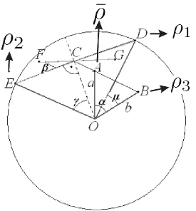
Figure 4: The Bloch representation of the three states $\{\rho_{1}=|\phi_{1}\rangle\langle\phi_{1}|,\rho_{2}=|\phi_{2}\rangle\langle\phi_{2}|,\rho_{3}\}$ and the parameters used in the proof of Proposition 9 are presented schematically in the Bloch ball. Two angles $(\alpha,\beta)$ characterize all possible triples $\{\rho_{1},\rho_{2},\rho_{3}\}$ if parameters $(a,b)$ are fixed.

Left hand side of Eq. (188) depends only on the lengths $a$ and $b$, and is independent of the concrete realization of the triple. Therefore to prove (188) for given $a$ and $b$ one has to find minimum of the entropy of the square root fidelity matrix over all triples parametrized by the angles $\alpha$ and $\beta$.

The entropy of the square–root fidelity matrix defined $G_{ij}=\sqrt{p_{i}p_{j}}\sqrt{F_{ij}}$ in Eq. (188) is a function of roots of the characteristic polynomial:

$$(\frac{1}{3}-\lambda)^{3}+p(\frac{1}{3}-\lambda)+q=0,$$ (190)

where

$$p = -(F_{12}+F_{13}+F_{23})/9$$ (191)

$$q = 2\sqrt{F_{12}F_{13}F_{23}}/27.$$ (192)

The parameter $p$ determines the second symmetric polynomial $s_{2}$ of eigenvalues of the square root fidelity matrix $G$

$$s_{2}=\frac{1}{9}\sum_{i<j}(1-F_{ij}).$$ (193)

The roots of equation (190) are equal to:

$$\lambda_{k}=\frac{1}{3}+2\sqrt{\frac{-p}{3}}\cos\Big{[}\Big{(}\frac{1}{3}\arccos{(\frac{3q}{2p}\sqrt{\frac{3}{-p}})}+k\frac{2\pi}{3}\Big{)}\Big{]},$$ (194)

where $k=1,...,3$.

The entropy of the square root fidelity matrix is a function of $p$ and $q$, which determine the second symmetric polynomial of eigenvalues (193) and the third symmetric polynomial is in this case equal to the determinant of the $3\times 3$ matrix $G_{ij}=\sqrt{p_{i}p_{j}}\sqrt{F_{ij}}$. The von Neumann entropy is a monotonically increasing function of all symmetric polynomials of eigenvalues [67]. The parameter $q$ is a function of $(a,b,\alpha,\beta)$, while parameter $p$ depends only on $a$ and $b$ which is shown in following lemma:

Lemma 2.

For any triple of two pure and one mixed state of an arbitrary dimension the sum of fidelities depends only on the purity of the mixed state and the barycenter of the ensemble.

Proof.

Denote by $\bar{\rho}$ the barycenter of a mixed state $\rho$ and two pure states, $\left|\phi_{1}\right\rangle$, $\left|\phi_{2}\right\rangle$,

$$\bar{\rho}=\frac{1}{3}\rho+\frac{1}{3}\left|\phi_{1}\right\rangle\left\langle\phi_{1}\right|+\frac{1}{3}\left|\phi_{2}\right\rangle\left\langle\phi_{2}\right|.$$ (195)

The purity of $\bar{\rho}$ is given by

$$\operatorname*{Tr}{\bar{\rho}^{2}}=\frac{1}{9}\Big{(}\operatorname*{Tr}{\rho^{2}}+2+2\left\langle\phi_{1}\right|\rho\left|\phi_{1}\right\rangle+2\left\langle\phi_{2}\right|\rho\left|\phi_{2}\right\rangle+2\left|\left\langle\phi_{1}\right|\left.\phi_{2}\right\rangle\right|^{2}\Big{)}.$$ (196)

After reordering the terms one gets

$$F_{12}+F_{13}+F_{23}=\frac{1}{2}(9\operatorname*{Tr}{\bar{\rho}^{2}}-\operatorname*{Tr}{\rho^{2}}-2),$$ (197)

where

$$F_{12}=\left|\left\langle\phi_{1}\right|\left.\phi_{2}\right\rangle\right|^{2},$$ (198)

$$F_{23}=\left\langle\phi_{2}\right|\rho\left|\phi_{2}\right\rangle,$$ (199)

$$F_{13}=\left\langle\phi_{1}\right|\rho\left|\phi_{1}\right\rangle.$$ (200)

Since $\operatorname*{Tr}\bar{\rho}^{2}=\frac{1}{2}(1+a^{2})$ and $\operatorname*{Tr}\rho^{2}=\frac{1}{2}(1+b^{2})$, the parameter $p$ defined in (191) does not depend on the angles $\alpha$ and $\beta$. This completes the proof of Lemma 2. ∎

The parameter $p$ and the second symmetric polynomial (193) does not depend on the angles $\alpha$ and $\beta$. Therefore, for given $a$ and $b$, the entropy of the square root fidelity matrix attains its minimum over $\alpha$ and $\beta$ for minimal value of the determinant of $G$, since the entropy is an increasing function of the determinant. The determinant is given by

$$\det{\left(\frac{1}{3}\begin{bmatrix}1&\sqrt{F_{12}}&\sqrt{F_{13}}\\ \sqrt{F_{21}}&1&\sqrt{F_{23}}\\ \sqrt{F_{31}}&\sqrt{F_{32}}&1\end{bmatrix}\right)}=\frac{1}{27}\left(1+2\sqrt{F_{12}F_{13}F_{23}}-(F_{12}+F_{13}+F_{23})\right).$$ (201)

It is the smallest for the smallest value of the parameter $q$ which is the function (192) of the off–diagonal elements of the matrix. During computations of the minimal value of $q$ another lemma will be useful:

Lemma 3.

Among triples of one–qubit states which realize the same barycenter, where one state is mixed of a given purity and two others are pure, the product of three pairwise fidelities is the smallest if three states and the average lie on the plane containing the great circle of the Bloch ball, i.e. $\beta=0$.

Proof.

The function $f(a,b,\alpha,\beta)=F_{12}F_{13}F_{31}$ is given explicitly in Appendix 2 based on Appendix 1. For given $a,b$ and $\alpha$ this function has minimum only at $\beta=0$ and equivalently for $\beta=\pi$. ∎

In consequence, searching for the minimum of the entropy of the square root fidelity matrix we can restrict our attention to the case $\beta=0$. In fact, for our purpose it suffices to take the specific value of $\alpha$ which is shown in the following lemma.

Lemma 4.

Among triples of one–qubit states which realize the same barycenter, in which one state is mixed of given purity and two others are pure, the product of three pairwise fidelities is the smallest when two pure states are symmetric with respect to the mixed state i.e. $\beta=0$ and $\alpha=0$ or $\alpha=\pi$.

Proof.

The function $f_{0}(a,b,\alpha,\beta=0)=F_{12}F_{13}F_{31}$ is given directly in Appendix 1. It has only one minimum at $\alpha=0$ but in certain cases, depending on $a$ and $b$, the value on the edge of variable range, i.e. at $\alpha=0$ or $\alpha=\pi$ is smaller. ∎

3.2.1 Proof of the fidelity bound

To prove inequality (188) the smallest entropy of the square root fidelity matrix for three states consistent with the left hand side of this inequality should be found. Entropy is a function of four parameters, $(a,b,\alpha,\beta)$. The left hand side of (188), which is the Holevo quantity depends on two parameters $(a,b)$ as follows

$$\chi=S\left(\frac{1}{2}\begin{bmatrix}1+a&0\\ 0&1-a\end{bmatrix}\right)-\frac{1}{3}S\left(\frac{1}{2}\begin{bmatrix}1+b&0\\ 0&1-b\end{bmatrix}\right).$$ (202)

For given parameters $a$ and $b$ lemmas 1, 2 and 3 allows us to find specific $\alpha$ and $\beta$ for which minimization of right hand side of (188) is obtained. One can fix $\alpha=0$ or $\alpha=\pi$ and $\beta=0$. That means, that minimal entropy of the square root fidelity $G$ over the angles is obtained if the three states $\{\rho_{1}=|\phi_{1}\rangle\langle\phi_{1}|,\rho_{2}=|\phi_{2}\rangle\langle\phi_{2}|,\rho_{3}\}$ are lying on the great circle and the two pure states are symmetric with respect to the mixed state. In this case the matrix $G$ is characterized by two parameters, $F=F_{12}=F_{23}$ and $b$. Here $F$ is the fidelity between the pure state $\rho_{1}$ and the mixed state $\rho_{3}$ whereas $b$ characterize the length of the Bloch vector of the mixed state $\rho_{3}$. The matrix $G$ reads

$$G=\frac{1}{3}\begin{pmatrix}1&\sqrt{F}&|\frac{2F-1}{b}|\\ \sqrt{F}&1&\sqrt{F}\\ |\frac{2F-1}{b}|&\sqrt{F}&1\end{pmatrix},$$ (203)

where $F$ is a function of $b$, such that $F(b)=\frac{1}{2}(1-bc)$, and $c$ is the length of the Bloch vector representing the barycenter of two pure states $\rho_{1}$ and $\rho_{2}$. The fidelity $F$ is equal to $1/2$ if $b$ tends to $0$. The parameter $c$ determines also the projection of the Bloch vector of the pure state $\rho_{1}$ on the Bloch vector of the mixed state $\rho_{3}$. The absolute value $|c|$ is equal to the square root fidelity between the two pure states. The range of variables are $0\leq b\leq 1$ and $\frac{1}{2}(1-b)\leq F\leq\frac{1}{2}(1+b)$.

Considered case is shown in Fig. 5. There are two surfaces – functions of two parameters $F$ and $b$. The lower surface represents the Holevo quantity $\chi$, and the upper surface denotes the entropy of the square root fidelity matrix (203). The surface $S(G)$ lies always above $\chi$ and is composed of two smooth functions characterizing cases in which all vectors lay on the same semicircle or pure states and the mixed state belong to the opposite semicircles.

Fig. 5 suggests that in the case of three pure states, $b=1$, laying on the same semicircle the inequality is saturated, $\chi=S(G)$. In this case, $F\geq 1/2$, the rank of the square root fidelity matrix is equal to $2$, and the nonzero eigenvalues are $(1\pm a)/2$, where $a=(4F-1)/3$ is the length of the Bloch vector of the average state $\bar{\rho}$. In general we have $a=\frac{1}{3}(b+2\frac{2F-1}{b})$. In case of $\chi=S(G)$ the Holevo quantity is equal to the entropy of the average state $\bar{\rho}$. This finishes the proof of Proposition 9.

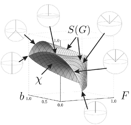
Figure 5: Evidence in favour of Proposition 9. The Holevo quantity as function of two variables: fidelity $F$ between the pure state $\rho_{1}$ and the mixed state $\rho_{3}$, and the length $b$ of the Bloch vector characterizing the state $\rho_{3}$. The upper surface representing the square root fidelity matrix $G$ is composed of two smooths parts. Every circle represents schematically the Bloch ball with exemplary positions of Bloch vectors characterizing three states $\{\rho_{1}=|\phi_{1}\rangle\langle\phi_{1}|,\rho_{2}=|\phi_{2}\rangle\langle\phi_{2}|,\rho_{3}\}$ of the ensemble.

Part III Minimal output entropy and map entropy

4 Entropies for one-qubit channels

The question on additivity of the channel capacity is one of the most interesting problems in quantum information theory [40]. Shor showed [39] that this problem has several equivalent formulations. One of them concerns the minimal output entropy,

$$S^{\min}(\Phi)=\min_{\rho}S(\Phi(\rho)).$$ (204)

In the case of one–qubit channel the minimal output entropy is the entropy of a state characterized by point on the ellipsoid, which is the image of the Bloch sphere, the closest to this sphere. The pure state which is transformed into a state of the minimal entropy is called minimizer.

For any setup in which minimal output entropy is additive the quantum channel capacity is additive as well. Additivity implies that an entangled state cannot increase capacity of two channels with respect to the sum of their capacities taken separately. The additivity conjecture can also be formulated as a statement that capacity of two channels is minimized for a product state.

The conjecture was confirmed in many special cases. For instance, additivity holds, if one of the channels is arbitrary and the second one is: bistochastic one–qubit map [87], a unitary transformation [40], generalized depolarizing channel [41], entanglement breaking channel [88], very noisy map [89] and others. A useful review on this subject was written by Holevo [90]. Different strategies of proving the additivity conjecture are analyzed there. For a recent relation on the additivity conjecture see also [18].

Also counterexamples to the additivity conjecture have been found. One of them was presented by Hastings [16]. He found the lower bound for the output entropy of some channels when the input was a product state. Next he estimated the output entropy for a maximally entangled input. Due to such estimations it was shown that the entangled state decreases channel capacity below the value achievable for product states.

The proof of Hastings used pairs of complementary channels. His argument was not constructive and works in high dimensional spaces. Counterexamples for the additivity hypothesis are also studied in [17].

It is still an open question, whether the additivity holds for an arbitrary one–qubit channel. Originally, the hypothesis on additivity of minimal output entropy was formulated for the von Neumann entropy. One of the approaches to the problem uses a one–parameter family of entropies, called Rényi entropies characterized by a parameter $q$,

$$S_{q}(\rho):=\frac{1}{1-q}\log\operatorname*{Tr}\rho^{q}.$$ (205)

Calculations are sometimes easier when the Rényi entropies are considered. The quantity $S_{q}$ tends to the von Neumann entropy in the limit $q\rightarrow 1$. Additivity of the minimal output Rényi entropy has been proved only in some range of the parameter $q$ depending on the channels considered [87, 41, 18].

Although the Rényi entropy is sometimes computationally more feasible, finding minimum over entire set of quantum states is still a hard problem. One of the ideas how to omit this difficulty tries to use some relations between minimal output entropy and other quantities which are easier to calculate. In the following chapter the Rényi entropy of a map (the map entropy) will be used to estimate the minimal output entropy. Map entropy (entropy of a map) is defined by the entropy of the Choi-Jamiołkowski state (28) corresponding to the map. This quantity is easy to obtain. Numerical tests presented in Fig. 7, 9, 10 show that there is no simple functional relation between the map entropy and the minimal output entropy. Nevertheless being aware of the structure of the set of quantum maps projected on the plane $(S^{\operatorname*{map}}_{q},S^{\min}_{q})$ can be useful. Knowledge of entropies of maps at the boundaries of the allowed set can be used to estimate the minimal output entropy by the entropy of the map.

4.1 Structure of the set of Pauli channels

Quantum channels which preserve the maximally mixed state are called bistochastic. All bistochastic one–qubit channels can be represented as a convex combination of the identity matrix $\sigma_{0}={\rm 1\rule{0.43057pt}{6.54443pt}\hskip 0.86108pt}$ and three Pauli matrices $\sigma_{i=1,2,3}$ (39)

$$\Phi_{\vec{p}}(\rho)=\sum_{i=0}^{3}p_{i}\sigma_{i}\rho\sigma_{i},\qquad\sum_{i=0}^{3}p_{i}=1,\qquad\forall_{i}p_{i}\geq 0.$$ (206)

Bistochastic one–qubit quantum operations are thus called Pauli channels. The structure of the set of all Pauli channels forms a regular tetrahedron $\Delta_{3}$ as shown in Fig. 6a. There are many channels characterized by the points of tetrahedron which can be obtained from other channels following a unitary transformation. Our considerations are often restricted to the asymmetric tetrahedron $K$ (see Fig. 6b) which is a subset of $\Delta_{3}$. All maps in $\Delta_{3}$ can be obtained from channels of $K$ by concatenation these channels with unitary transformations. The set $K$ is formed by the convex combination of four vectors $\vec{p}$ from (206), $A=(0,0,0,0),\ B=(1/2,1/2,0,0),\ C=(1/3,1/3,1/3,0)$, and $D=(1/4,1/4,1/4,1/4)$.

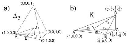
Figure 6: The structure of one–qubit bistochastic quantum operations corresponds to the regular tetrahedron $\Delta_{3}$. This figure is spanned by four extremal vectors $\vec{p}$ from formula (206). Symmetries of the tetrahedron allow us to distinguish the asymmetric set $K$ inside $\Delta_{3}$. Any vector $\vec{p}$ characterizing a Pauli channel can be obtained by permutation of elements of vectors from $K$.

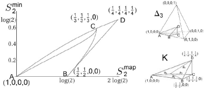
Figure 7: Lines $AB$, $BD$ and $AD$, which correspond to the edges of asymmetric tetrahedron $K$ form the boundaries of the entire set of Pauli matrices projected on the plane $(S^{\operatorname*{map}}_{2},S^{\min}_{2})$.

Extremal lines of the asymmetric tetrahedron correspond to the following families of maps: $AB$ - dephasing channels, $BD$ - classical bistochastic maps, $AD$ and $CD$ - depolarizing channels. The families mentioned above are also shown in Fig. 7 which presents boundaries of the set of all one–qubit bistochastic channels projected onto the plane $(S_{2}^{\operatorname*{map}},S_{2}^{\min})$. A following proposition proved in [51] characterizes this projection.

Proposition 10.

Extremal lines of asymmetric tetrahedron correspond to boundaries of the set of all bistochastic one–qubit maps on the plot $(S_{2}^{\operatorname*{map}},S_{2}^{\min})$.

4.2 Depolarizing channels

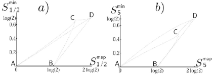
Figure 10: As in Fig. 9a: projection of the set of Pauli channels onto the plane spanned by the Rényi entropy of a map $S_{q}^{\operatorname*{map}}$ and the minimal Rényi output entropy $S_{q}^{\min}$ obtained for $a)$ $q=1/2$ and $b)$ $q=5$.

Fig. 9 and Fig. 10 show the projection of the Pauli channels on the plane $(S_{q}^{\operatorname*{map}},S_{q}^{\min})$ with parameter $q$ different than $2$. Comparison of these figures with Fig. 7 shows that the structure of the set of channels on the plane $(S_{q}^{\operatorname*{map}},S_{q}^{\min})$ is the simplest in case of the Rényi entropy of order $q=2$. In this case, the depolarizing channels form one of the edges of the set of all quantum one–qubit maps projected onto the plane. Indeed the following theorem proved in [51] confirms the special role of depolarizing channels in the set of all quantum channels acting on states of arbitrary dimension $N$.

Theorem 6.

Depolarizing channels have the smallest map Rényi entropy $S_{2}^{\operatorname*{map}}$ among all channels with the same minimal output Rényi entropy $S_{2}^{\min}$.

The family of depolarizing channels is represented in the plane $(S_{2}^{\operatorname*{map}},S_{2}^{\min})$ by the continuous line on the entire range of $S_{2}^{\operatorname*{map}}$. The minimal output entropy of a depolarizing channel $\Lambda_{N}$ acting on $\mathcal{M}_{N}$ is the following function of the map entropy

$$S_{2}^{\mathrm{min}}\Big{(}S_{2}^{\mathrm{map}}(\Lambda_{N})\Big{)}=-\log\Big{(}\frac{1+N\mathrm{e}^{-S_{2}^{\mathrm{map}}(\Lambda_{N})}}{N+1}\Big{)}.$$ (207)

This is a monotonously increasing function from $0$ to $\log{N}$. Therefore the following theorem holds.

Theorem 7.

Depolarizing channels have the greatest minimal output Rényi entropy $S_{2}^{\min}$ among all maps of the same Rényi entropy of a map $S_{2}^{\operatorname*{map}}$.

One can try to use the extremal position of depolarizing channels to estimate the minimal output entropy of some channels. In the case of Hastings’ counterexample for the additivity conjecture the author showed that due to a maximally entangled input state one can obtain smaller output entropy of the product of two channels than in the case of any product state taken as an input. Let us estimate the Rényi $q=2$ output entropy for a product channel when the input is maximally entangled. Following proposition proved in [51] presents one of estimations.

Proposition 11.

For any entropy $\mathcal{S}$ which is subadditive the following inequality holds

$$|\mathcal{S}^{\operatorname*{map}}(\Phi_{1})-\mathcal{S}^{\operatorname*{map}}(\Phi_{2})|\leq\mathcal{S}\Big{(}[\Phi_{1}\otimes\Phi_{2}](|\phi_{+}\rangle\langle\phi_{+}|)\Big{)}\leq\mathcal{S}^{\operatorname*{map}}(\Phi_{1})+\mathcal{S}^{\operatorname*{map}}(\Phi_{2}),$$ (208)

where $|\phi_{+}\rangle\langle\phi_{+}|$ is a maximally entangled state.

Proof.

The proof starts form the Lindblad inequality [75], which is based on the subadditivity of the von Neumann entropy,

$$\bigl{|}\mathcal{S}(\rho)-\mathcal{S}\big{(}\varsigma(\Phi,\rho)\big{)}\bigr{|}\leq\mathcal{S}(\Phi(\rho))\leq\mathcal{S}(\rho)+\mathcal{S}\big{(}\varsigma(\Phi,\rho)\big{)},$$ (209)

where $\varsigma(\Phi,\rho)=[\operatorname{id}\otimes\Phi]\Big{(}|\phi\rangle\langle\phi|\Big{)}$ and $|\phi\rangle$ is a purification of $\rho$ as in (106). The entropy of this state, $S(\varsigma(\Phi,\rho))$, is the exchange entropy which does not depend on the choice of purification [29]. The state $\varsigma$ defined for a channel $\Phi$ and the maximally mixed state $\rho_{*}={\rm 1\rule{0.43057pt}{6.54443pt}\hskip 0.86108pt}/N$ is equal to the normalized dynamical matrix of $\Phi$ (25),

$$\varsigma(\Phi,\rho_{*})=\sigma_{\Phi}=\frac{1}{N}D_{\Phi},$$ (210)

The entropy of this state defines $\mathcal{S}^{\operatorname*{map}}(\Phi)$. Since the map $\Phi$ is trace preserving, the condition ${\rm Tr}_{2}\sigma_{\Phi}=\frac{1}{N}{\rm 1\rule{0.43057pt}{6.54443pt}\hskip 0.86108pt}$ holds, see (26). Apply Lindblad formula (209) to the state

$$[\Phi_{1}\otimes\Phi_{2}](|\psi_{+}\rangle\langle\psi_{+}|)=[\Phi_{1}\otimes\operatorname{id}]\left([\operatorname{id}\otimes\Phi_{2}](|\psi_{+}\rangle\langle\psi_{+}|)\right),$$ (211)

where $|\psi_{+}\rangle=\frac{1}{\sqrt{N}}\sum_{i=1}^{N}|i\rangle\otimes|i\rangle$ is the maximally mixed state which is a purification of $\rho_{*}$. Expression (209) applied to this state gives

$$\bigl{|}\mathcal{S}^{\mathrm{map}}(\Phi_{2})-\mathcal{S}\bigl{(}\varsigma(\Phi_{1}\otimes\operatorname{id},\,\sigma_{\Phi_{2}})\bigr{)}\bigr{|} \leq \mathcal{S}\bigl{(}(\Phi_{1}\otimes\Phi_{2})(|\psi_{+}\rangle\langle\psi_{+}|)\bigr{)}$$

$$\leq \mathcal{S}^{\mathrm{map}}(\Phi_{2})+\mathcal{S}\bigl{(}\varsigma(\Phi_{1}\otimes\operatorname{id},\,\sigma_{\Phi_{2}})\bigr{)}.$$

The exchange entropy $\mathcal{S}\bigl{(}\varsigma(\Phi_{1}\otimes\operatorname{id},\,\sigma_{\Phi_{2}})\bigr{)}$ is the same as $\mathcal{S}\bigl{(}\varsigma(\Phi_{1},\,\operatorname*{Tr}_{2}\sigma_{\Phi_{2}})\bigr{)}$ since a purification of $\sigma_{\Phi_{2}}$ is as well the purification of $\operatorname*{Tr}_{2}\sigma_{\Phi_{2}}$ and the exchange entropy does not depend on a purification. Due to the trace preservation formula, $\operatorname*{Tr}_{2}\sigma_{\Phi_{2}}=\rho_{*}$, the state $\varsigma(\Phi_{1},\,\operatorname*{Tr}_{2}\sigma_{\Phi_{2}})=\varsigma(\Phi_{1},\,\rho_{*})=\sigma_{\Phi_{1}}$ which completes the proof. ∎

Proposition 11 is applicable for any entropy which is subadditive. The Rényi entropy of order $q=2$ is not subadditive, however, it is a function of the Tsallis entropy of order $2$ for which the subadditivity holds. Therefore Proposition 11 can be used to estimate the output Rényi $q=2$ entropy of a product channel if the input state is maximally entangled. The following inequality corresponds to Rényi $q=2$ version of the lower bound in (208),

$$-\log\Big{(}1-|e^{-S_{2}^{\operatorname*{map}}(\Phi_{1})}-e^{-S_{2}^{\operatorname*{map}}(\Phi_{2})}|\Big{)}\leq S_{2}\Big{(}(\Phi_{1}\otimes\Phi_{2})(|\psi_{+}\rangle\langle\psi_{+}|)\Big{)}.$$ (213)

It is possible to find channels $\Phi_{1}$ and $\Phi_{2}$ such that the left hand side of (213) is greater than $S^{\min}_{2}$ of depolarizing channel $\Lambda$, which has the same map entropy as $S_{2}^{\operatorname*{map}}(\Phi_{1}\otimes\Phi_{2})$. Notice that for any two channels the map entropy of their tensor product is characterized by the following result.

Proposition 12.

The Rényi map entropy $S_{q}^{\operatorname*{map}}$ is additive with respect to tensor product of quantum maps for any parameter $q\geq 0$:

$$S_{q}^{\operatorname*{map}}(\Phi_{1}\otimes\Phi_{2})=S_{q}^{\operatorname*{map}}(\Phi_{1})+S_{q}^{\operatorname*{map}}(\Phi_{2}).$$ (214)

Proof.

The map entropy $S_{q}^{\operatorname*{map}}(\Phi)$ is defined as the entropy of normalized dynamical matrix $D_{\Phi}$. The matrix representation of $D_{\Phi_{1}\otimes\Phi_{2}}$ is related to superoperator matrix of the quantum operation $\Phi_{1}\otimes\Phi_{2}$, due to formula (28). Using explicit calculations on matrix elements one can show that $D_{\Phi_{1}\otimes\Phi_{2}}$ is unitarily equivalent with $D_{\Phi_{1}}\otimes D_{\Phi_{2}}$. That implies the additivity of the map entropies, since the quantum Rényi entropy of any order of a given state is a function of its spectrum.

Consider a set of $N$-dimensional matrices equipped with the Hilbert-Schmidt inner product

$$\langle A|B\rangle_{\mathbf{h}}:=\operatorname*{Tr}A^{\dagger}B.$$ (215)

In this space the matrix units $\bigl{\{}|i\rangle\langle j|\,\bigm{|}\,i,j=1,2,\ldots,N\bigr{\}}$ form an orthonormal basis. The elements of this basis are denoted by $|i\rangle\langle j|:=|ij\rangle_{\mathbf{h}}$. A quantum operation $\Phi$ is represented by a matrix $\hat{\Phi}$:

$$\langle ij|\hat{\Phi}|k\ell\rangle_{\mathbf{h}}=\operatorname*{Tr}\Bigl{(}|j\rangle\langle i|\,\Phi(|k\rangle\langle\ell|)\Bigr{)},$$ (216)

hence

$$\Phi(|k\rangle\langle\ell|)=\sum_{i,j}\langle ij|\hat{\Phi}|k\ell\rangle_{\mathbf{h}}\,|i\rangle\langle j|.$$ (217)

Due to the reshuffling procedure (28), the entries of the dynamical matrix $D_{\Phi}$ read

$$\langle ab|D_{\Phi}|cd\rangle_{\mathbf{h}}=\langle ac|\hat{\Phi}|bd\rangle_{\mathbf{h}}.$$ (218)

The entries of $D_{\Phi_{1}\otimes\Phi_{2}}$ are obtained by using unnormalized maximally entangled state $|\Psi_{+}\rangle:=\sum_{i,\ell}|i\ell\rangle\otimes|i\ell\rangle$ according to definition (25) as follows

$$\,\langle abcd|D_{\Phi_{1}\otimes\Phi_{2}}|efgh\rangle =\langle abcd|\bigl{[}(\Phi_{1}\otimes\Phi_{2})\otimes\operatorname{id}\bigr{]}\bigl{(}|\Psi_{+}\rangle\langle\Psi_{+}|\bigr{)}|efgh\rangle$$

$$=\sum_{i,\ell,j,m}\langle abcd|\bigl{[}(\Phi_{1}\otimes\Phi_{2})(|i\ell\rangle\langle jm|)\otimes|i\ell\rangle\langle jm|\bigr{]}|efgh\rangle.$$ (219)

Now expression (217) is used and the matrix elements of $D_{\Phi_{1}\otimes\Phi_{2}}$ read

$$\langle abcd|D_{\Phi_{1}\otimes\Phi_{2}}|efgh\rangle=\sum_{\alpha,\beta,\gamma,\delta}\langle\alpha\beta|\widehat{\Phi_{1}}|ij\rangle_{\mathbf{h}}\,\langle\gamma\delta|\widehat{\Phi_{2}}|ij\rangle_{\mathbf{h}}\,\langle abcd|\alpha\gamma i\ell\rangle\,\langle\beta\delta jm|efgh\rangle.$$ (220)

Since $\langle abcd|\alpha\gamma i\ell\rangle$ is expressed in terms of Kronecker deltas $\delta_{a\alpha}\delta_{b\gamma}\delta_{ci}\delta_{d\ell}$ and $\langle\beta\delta jm|efgh\rangle$ analogously, the summation over the Greek indexes gives,

$$\langle abcd|D_{\Phi_{1}\otimes\Phi_{2}}|efgh\rangle =\langle ac|D_{\Phi_{1}}|eg\rangle\,\langle bd|D_{\Phi_{2}}|fh\rangle$$

$$=\langle acbd|D_{\Phi_{1}}\otimes D_{\Phi_{2}}|egfh\rangle.$$ (221)

The matrix $D_{\Phi_{1}\otimes\Phi_{2}}$ is related to $D_{\Phi_{1}}\otimes D_{\Phi_{2}}$ by a unitary matrix
$U=\sum_{a,b,c,d}|abcd\rangle\langle acbd|$. Therefore both matrices have the same eigenvalues and the same entropies. ∎

Since minimal output entropy of a depolarizing channel $\Lambda$ is a function of its map entropy (207), the estimation on the left hand side of (213) can be made in terms of such $\Lambda$ for which $S_{2}^{\operatorname*{map}}(\Lambda)=S_{2}^{\operatorname*{map}}(\Phi_{1})+S_{2}^{\operatorname*{map}}(\Phi_{2})$. As a result of this estimation one obtains condition on the pair of channels, for which a maximally mixed input state does not decrease the output entropy below the smallest value obtained by the product input state,

$$1-\frac{MN+1}{MN}|e^{-S_{2}^{\operatorname*{map}}(\Phi_{1})}-e^{-S_{2}^{\operatorname*{map}}(\Phi_{2})}|\leq e^{-S_{2}^{\operatorname*{map}}(\Phi_{1}\otimes\Phi_{2})}=e^{-\big{[}S_{2}^{\operatorname*{map}}(\Phi_{1})+S_{2}^{\operatorname*{map}}(\Phi_{2})\big{]}},$$ (222)

where $\Phi_{1}$ acts on $\mathcal{M}_{N}$ and $\Phi_{1}$ on $\mathcal{M}_{M}$.

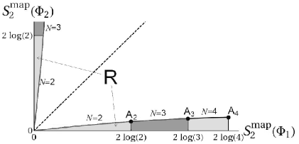
Figure 8: Colored parts of the figure denote the region described by inequality (222). This region contains pairs of maps characterized by their map entropy for which the additivity is conjectured. The dotted line contains the pairs of complementary channels. The region is enlarged if a larger dimensions are considered.

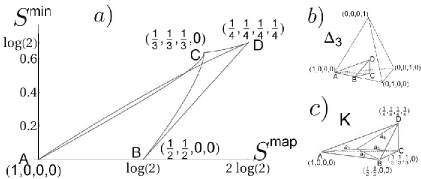
Figure 9: The set of the Pauli channels projected on the plane spanned by the map entropy $S^{\operatorname*{map}}$ and the minimal output entropy $S^{\min}$. The von Neumann entropies are considered. Solid curves correspond to the edges of the asymmetric tetrahedron K. The curve AD characterizing the family of depolarizing channels does not belong to the boundary of the set.

Fig. 8 presents the region defined by (222). Such a set is not empty and contains maps, for which $S^{\operatorname*{map}}_{2}(\Phi_{1})<<S^{\operatorname*{map}}_{2}(\Phi_{2})$ or $S^{\operatorname*{map}}_{2}(\Phi_{2})<<S^{\operatorname*{map}}_{2}(\Phi_{1})$. The dotted line represents the set of complementary channels for which both map entropies are equal. This set contains the channels breaking the conjecture of additivity of minimal output entropy according to the proof of Hastings. The region defined by (222) does not intersect the set. It was also shown [40], [89] that additivity holds if one of the channels is unitary or if one of the channels is very noisy. These both cases are covered by condition (222). These examples support formulation of

Conjecture 2 ([51]).

The additivity of minimal output Rényi $q=2$ entropy holds for pair of channels satisfying inequality (222).

Recent literature does not answer the question, whether the additivity conjecture is broken for low dimensional channels and the Rényi entropy of order $q=2$. Our Conjecture 2 suggests for which pairs of channels finding a counterexample of additivity is unlikely.

Conjecture 2 uses the map entropy and is formulated for the Rényi entropy of order $2$, for which the theorem about extremal position of the depolarizing channels was proved. This is the key theorem which allows us to derive estimations (213) and (222). Numerical tests (Fig. 9 and 10) suggest that the depolarizing channels are not situated at the boundary of the set of all channels in the plane $(S_{q}^{\operatorname*{map}},S_{q}^{\min})$ for $q\leq 2$, while their extremal position could be confirmed in case $q\geq 2$. Nevertheless, the Rényi entropy is a smooth function of $q$. Therefore, a conjecture similar to Conjecture 2 may hold also for other values of the Rényi parameter $q$.

4.3 Transformations preserving minimal output entropy

In previous chapter the set of one–qubit quantum operations was considered in context of the plot $(S_{q}^{\operatorname*{map}},S_{q}^{\min})$. One could ask, whether the family of maps lying at the same vertical or horizontal line can be characterized. The following section gives a partial answer to this question. Transformations of one qubit maps which preserve the minimal output entropy will be considered. Such a transformation changes the quantum channel and moves the corresponding point in the plane $(S_{q}^{\operatorname*{map}},S_{q}^{\min})$ along a given horizontal line. In the following section we consider the geometrical picture of one–qubit maps acting on the set of pure states. One–qubit quantum operation transforms the Bloch ball into an ellipsoid inside the ball. A transformation of quantum operation which changes the lengths of the axes of the ellipsoid and their orientation and leaves the minimal output entropy unchanged will be studied.

Consider the superoperator matrix of a one–qubit quantum operation:

$$\Phi=\begin{pmatrix}\Phi_{11}&\Phi_{12}&\overline{\Phi_{12}}&\Phi_{14}\\ \Phi_{21}&\Phi_{22}&\overline{\Phi_{32}}&\Phi_{24}\\ \overline{\Phi_{21}}&\Phi_{32}&\overline{\Phi_{22}}&\overline{\Phi_{34}}\\ 1-\Phi_{11}&-\Phi_{12}&-\overline{\Phi_{12}}&1-\Phi_{14}\end{pmatrix}.$$ (223)

Parameters $\Phi_{11}$ and $\Phi_{14}$ are real, the complex conjugation of $\Phi_{ij}$ is denoted by $\overline{\Phi_{ij}}$. The form (223) guarantees that the dynamical matrix of $\Phi$ is Hermitian and the trace preserving condition (26) is satisfied.

Assume that the quantum operation $\Phi_{1}$ has the output entropy minimizer at the point

$$\rho_{p}=\begin{pmatrix}p&\sqrt{p(1-p)}\\ \sqrt{p(1-p)}&1-p\end{pmatrix}.$$ (224)

Such an assumption is not restrictive since one can always treat the operation $\Phi_{1}$ as a concatenation of a given operation with a unitary rotation which does not change the minimal output entropy. The quantum operation (223) acting on a pure state

$$\rho_{in}=\begin{pmatrix}a&\sqrt{a(1-a)}\\ \sqrt{a(1-a)}&1-a\end{pmatrix}$$ (225)

gives an output state

$$\rho_{out}\ \ = a\begin{pmatrix}\Phi_{11}&\Phi_{21}\\ \overline{\Phi_{21}}&1-\Phi_{11}\end{pmatrix}+(1-a)\begin{pmatrix}\Phi_{14}&\Phi_{24}\\ \overline{\Phi_{24}}&1-\Phi_{14}\end{pmatrix}+$$ (226)

$$+\sqrt{a(1-a)}\begin{pmatrix}2\Re(\Phi_{12}e^{i\phi})&\Phi_{22}e^{i\phi}+\overline{\Phi_{32}}e^{-i\phi}\\ \overline{\Phi_{22}}e^{-i\phi}+\Phi_{32}e^{i\phi}&-2\Re(\Phi_{12}e^{i\phi})\end{pmatrix},$$

which attains the minimum entropy if $a=p$.

• Transformation changing the lengths of the axes of the ellipsoid.

  Consider a quantum operation $\Phi_{ellipsoid}$, which transforms the Bloch ball into such an ellipsoid that the end of its longest axis touches the Bloch sphere in the "North Pole",

  $$\Phi_{ellipsoid}=\left(\begin{array}[]{cccc}1&0&0&1-\text{$\eta$3}\\ 0&\frac{\text{$\eta_{1}$}+\text{$\eta_{2}$}}{2}&\frac{\text{$\eta_{1}$}-\text{$\eta_{2}$}}{2}&0\\ 0&\frac{\text{$\eta_{1}$}-\text{$\eta_{2}$}}{2}&\frac{\text{$\eta_{1}$}+\text{$\eta_{2}$}}{2}&0\\ 0&0&0&\text{$\eta_{3}$}\end{array}\right).$$ (227)

  Suitable rotations of the Bloch ball before and after the action of $\Phi_{ellipsoid}$ guarantees that the point of contact with the Bloch sphere is the minimizer of $\Phi_{1}$. Therefore the concatenation of $\Phi_{1}\cdot\Phi_{rotation}\cdot\Phi_{ellipsoid}\cdot\Phi_{rotation}$ has the same minimal output entropy and the same minimizer that $\Phi_{1}$. The rotation operation is given by

  $$\Phi_{rotation}=\left(\begin{array}[]{cccc}p&-\sqrt{(1-p)p}&-\sqrt{(1-p)p}&1-p\\ \sqrt{(1-p)p}&p&p-1&-\sqrt{(1-p)p}\\ \sqrt{(1-p)p}&p-1&p&-\sqrt{(1-p)p}\\ 1-p&\sqrt{(1-p)p}&\sqrt{(1-p)p}&p\end{array}\right),$$ (228)

  where $p$ is defined by the minimizer of output entropy for $\Phi_{1}$. This transformation changes the lengths of axes of the ellipsoid but it does not change the point at the ellipsoid which is the closest to the Bloch sphere. In other words, this transformation does not change the directions of the axes of the image of $\Phi_{1}$ into the Bloch ball, but only their lengths.

• Transformation changing directions of the axis.

  The next transformation changes directions of axes of an ellipsoid but preserves the entropy minimizer. In particular, if the image of the minimizer is on the longest axis of an ellipsoid, after the transformation the point which is the closest to the Bloch sphere is no longer on the main axis of the ellipsoid.

  Entropy of an output state (226) is a function of its determinant. The minimum of the determinant determines the minimum of the entropy. Consider a transformation which preserves the value of the determinant and compute its derivative in a minimizer. It is useful to introduce the compact notation of Eq. (226):

  $$\rho_{out}=aA+(1-a)B+\sqrt{a(1-a)}C,$$ (229)

  where matrices $A,B$ and $C$ correspond to the matrices (226). Consider a transformation $\Phi_{1}\rightarrow\Phi_{1}+\Phi_{direction}$. The output of $\Phi_{1}+\Phi_{direction}$ is given by

  $$\rho^{\prime}=a(A+\frac{1}{2}\frac{\sqrt{1-p}}{\sqrt{p}}X)+(1-a)(B+\frac{1}{2}\frac{\sqrt{p}}{\sqrt{1-p}}X)+\sqrt{a(1-a)}(C-X),$$ (230)

  where $X$ is a matrix, which is hermitian and has trace equal to zero. Moreover, the matrix $X$ satisfies the condition guaranteeing that $\Phi_{1}+\Phi_{direction}$ is completely positive. The state $\rho^{\prime}$ coincides with (229) if $a=p$. Moreover, the derivative of formula (229) with respect to $a$ is the same as the derivative of Eq. (230) at the point $a=p$. Therefore, the determinants of (229) and (230) are the same and the derivative at $a=p$ is equal to zero. A proper choice of parameters in $X$ guarantees that there is a minimum at point $a=p$. Hence both maps, $\Phi_{1}$ and $\Phi_{1}+\Phi_{direction}$ have the same minimal output entropy.

  The part $\Phi_{direction}$ can be characterized by two parameters $(t,n)$,

  $$\Phi_{direction}=\frac{1}{2}\left(\begin{array}[]{cccc}\sqrt{\frac{1-p}{p}}\ t&-t&-t&\sqrt{\frac{p}{1-p}}\ t\\ i\sqrt{\frac{1-p}{p}}\ n&-i\ n&-i\ n&i\sqrt{\frac{p}{1-p}}\ n\\ -i\sqrt{\frac{1-p}{p}}\ n&i\ n&i\ n&-i\sqrt{\frac{p}{1-p}}\ n\\ -\sqrt{\frac{1-p}{p}}\ t&t&t&-\sqrt{\frac{p}{1-p}}\ t\end{array}\right).$$ (231)

Such a form guarantees that the output state of $\Phi_{1}+\Phi_{direction}$ is given by Eq. (230).

The map $\Phi_{2}$ of the same minimal output entropy as $\Phi_{1}$ obtained by joint action of three transformations, $\Phi_{rotation}$, $\Phi_{ellipsoid}$ and $\Phi_{direction}$, on $\Phi_{1}$ can be given by:

$$\Phi_{2}=\Phi_{1}\Phi_{rotation}\cdot\Phi_{ellipsoid}\cdot\Phi^{T}_{rotation}+\Phi_{direction}.$$ (232)

We are not able to prove that this transformation contains all possibilities of obtaining maps with the same minimal output entropy as a given one, however, the transformation is characterized by $5$ parameters and also $5$ parameters are needed to have all different (up to one rotation) ellipsoids tangent to the sphere on its inner side in a given point. Three parameters are associated with the lengths of axes $|\eta_{1}|,|\eta_{2}|,|\eta_{3}|$, while two parameters define the direction of the longest axis $n,t$.

Above considerations introduce a $5$-parameter transformation of a quantum map $\Phi_{1}\rightarrow\Phi_{2}$. The transformation preserves the minimal output entropy. Therefore, it determines the family of maps which are situated at the same horizontal line of the plot $(S^{\operatorname*{map}},S^{\min})$. Characterization of the family of quantum maps parametrized by the minimal output entropy can be useful to further investigations of relations between $S^{\min}$ and $S^{\operatorname*{map}}$ and their consequences.

5 Davies maps for qubits and qutrits

Explicit description of general continuous dynamics of an open quantum system is difficult in practice. Exact formulas describing the time evolution are known in some special cases only. One of the cases in which the problem can be solved uses the assumption of a week coupling [91] of a low dimensional quantum system interacting with much bigger reservoir in the thermal equilibrium. Such an interaction changes only the state of the system whereas the state of the environment remains unchanged. By analogy to the classical process, in which the evolution of a state does not depend on the history, such an evolution is called a Markov process.

However, while analysing the continuous evolution of the input state, sometimes there is no need to know the entire time evolution since only the output state is relevant. The "black box" description is useful in such cases. A "black box" acts like an evolution discrete in time and can be described using completely positive maps, represented as matrices of superoperators.

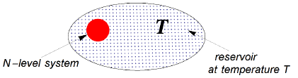
Figure 11: Model of a quantum $N$–level system characterized by Hamiltonian $H$ interacting with a much larger environment in a thermal equilibrium at temperature $T$.

The following chapter distinguishes a concrete class of physical processes described by a Davies map [92]. Such a process is compatible with the interaction of a quantum state with an environment in a given temperature, see Fig. 11. Due to a suitable choice of the entries of a superoperator matrix $\Phi$ and relations between them one can say whether some continuous time evolution is described by a given discrete quantum map. The solution concerns the maps acting on one–qubit, $N=2$, and one–qutrit, $N=3$. In the case of one-qubit maps we determine the state which is the most resistant on Davies channels. It will be shown that the maximal output $2$–norm of Davies maps is additive with respect to the tensor product of two such maps.

5.1 Quantum Markov process

The quantum Markov process is characterized by quantum maps belonging to the one-parameter completely positive semigroup, $\Phi_{t}=\exp{\mathcal{G}t}$, where $\mathcal{G}$ denotes a generator and positive parameter $t$ is associated with time.

The most general form of the generator of a completely positive semigroup was given by Gorini, Kossakowski, Sudarshan [93] and Lindblad [43]. It can be written as

$$\mathcal{G}=i\delta+\mathcal{L},$$ (233)

where $\delta$, given by the commutator with the effective Hamiltonian of the system $\delta:\rho\rightarrow[\rho,H]$, describes the unitary part of the evolution. The dissipative part $\mathcal{L}$ has the Lindblad form

$$\mathcal{L}:\rho\rightarrow\sum_{\alpha}\Big{(}K^{\alpha}\rho K^{\alpha\dagger}-\frac{1}{2}\{K^{\alpha\dagger}K^{\alpha},\rho\}\Big{)},$$ (234)

where $\{A,B\}=AB+BA$ is anticommutator, while operators $K^{\alpha}$ can be associated with the Kraus representation of the quantum operation.

Deciding whether a given superoperator matrix belongs to the completely positive semigroup was shown [94] to be a problem ’NP’ hard with respect to the dimension $N$. Nevertheless, some additional assumptions allow one to characterize matrices from completely positive semigroups at least for a few low dimensions. In following chapter, such a solution will be given for $N=2$, and $N=3$, under additional conditions: independence of unitary and dissipative parts of the evolution and the detailed balance condition. These three conditions define the so–called Davies maps [92]. Sometimes the uniqueness of the invariant state is also added to the definition.

5.2 Characterization of the model

Consider a quantum $N$ - level system characterized by the Hamiltonian in its eigenbasis,

$$H=\sum_{i=1}^{N}\epsilon_{i}|i\rangle\langle i|.$$ (235)

Assume that such a system is weekly coupled to the environment of a given temperature $T$, see Fig. 11. An interaction with the environment preserves one invariant state, which is the Gibbs state

$$\rho_{\beta}=\frac{1}{\mathcal{Z}}\exp(-\beta H),$$ (236)

where $\mathcal{Z}=\sum_{i=1}^{N}\exp(-\beta\epsilon_{i})$ is a partition function and $\beta=\frac{1}{kT}$. Here $k$ represents the Boltzmann constant. A quantum map $\Phi$ satisfies the detailed balance condition if it is Hermitian with respect to the scalar product defined by the Gibbs state

$$\operatorname*{Tr}\rho_{\beta}A\Phi^{*}(B)=\operatorname*{Tr}\rho_{\beta}\Phi^{*}(A)B,$$ (237)

where $A$ and $B$ are arbitrary observables and $\Phi^{*}$ the quantum operation in the Heisenberg picture. Detailed description of this condition can be found in [96].

The name "detailed balance" was taken from the theory of stochastic processes. Detailed balance means that in an equilibrium state any two levels of the evolving system remain in an equilibrium: the rate of transition from the level $i$ to $j$ and the transition rate from $j$ to $i$ are equal. Mathematical formula describing this fact reads

$$\mathcal{F}_{ij}p_{i}=\mathcal{F}_{ji}p_{j},$$ (238)

where $\mathcal{F}_{ij}$ are entries of a stochastic transition matrix and $p_{i}$ represent the components of the invariant probability vector.

5.3 Matrix representation of Davies maps

One qubit map in the "black box" description is represented by a superoperator matrix. It is a matrix acting on the vector formed by the entries of a density matrix ordered in a single column. A superoperator $\Phi$ represents a Davies map, if the following conditions are satisfied.

• The map $\Phi$ is completely positive.

  This condition is guaranteed if the Choi–Jamiołkowski matrix $D_{\Phi}$ (25) of the map is positive. One has to reshuffle the elements of the matrix $\Phi$ according to (28) and check positivity of the resulting dynamical matrix $D_{\Phi}=\Phi^{R}$.

• Superoperator $\Phi$ belongs to the semigroup of completely positive maps.

  This is equivalent to existence of a generator $\mathcal{G}$ of the Lindblad form (234) and the parameter $t\geq 0$ such that $\mathcal{G}t=\log\Phi$. Knowing the logarithm of $\Phi$ one has to determine whether it is of the Lindblad form. It was shown in [95] that if the Choi-Jamiołkowski matrix of a given generator is positive in the subspace orthogonal to the maximally entangled state, then the generator can be written in the Lindblad form.

  It is not a trivial task to write an analytical expression for the logarithm of a given matrix if its dimension is greater than two. Such a problem for $3\times 3$ stochastic matrices is discussed in the last section of the following chapter.

• Since the rotational part of the evolution is independent of the dissipative (contractive) part, the structure of the superoperator is restricted to the block diagonal form. Off–diagonal elements of the density matrix are just multiplied by numbers, while the diagonal elements can be mixed between themselves. More detailed discussion on this property is given in Section 5.7.

• The detailed balance condition introduces further restrictions on the elements of the block acting on the diagonal part of the density matrix. This block is a stochastic matrix, the entries of which satisfy Eq. (238).

Since now, only the dissipative part of the evolution will be considered. Due to the above conditions the dissipative part of the generator of the one–qubit Davies maps can be written as

$$\mathcal{L}_{\alpha,\lambda,p}=\begin{pmatrix}-\alpha&0&0&\alpha\frac{p}{1-p}\\ 0&\lambda&0&0\\ 0&0&\lambda&0\\ \alpha&0&0&-\alpha\frac{p}{1-p}\end{pmatrix},$$ (239)

while the corresponding superoperator acting on two-dimensional states (in the Hamiltonian basis) has the form

$$\Phi_{a,c,p}=\begin{pmatrix}1-a&0&0&a\frac{p}{1-p}\\ 0&c&0&0\\ 0&0&c&0\\ a&0&0&1-a\frac{p}{1-p}\end{pmatrix}.$$ (240)

Here, $p$ is a function of temperature, $p=\big{(}1+\exp{(-\frac{\epsilon}{(kT}})\big{)}^{-1}$, which determines the invariant state

$$\Phi_{a,c,p}(\rho_{*})=\rho_{*}=\begin{pmatrix}p&0\\ 0&1-p\end{pmatrix}.$$ (241)

Notice that (240) has a block diagonal form which is a consequence of independence of rotational and contractive evolution. This is also equivalent to independence of changes in diagonal and off–diagonal entries of a density matrix. The detailed balance condition $(\ref{cdetbal})$ implies the form of the outer block in Eq. (240). One–qubit Davies maps form a three-parameter family characterized by $(a,c,p)$, where $p$ is a function of the temperature. Conditions that such a matrix is an element of the semigroup of completely positive maps introduce the following restrictions on the parameters $(a,c,p)$:

$$a+p<1,\qquad 0<c<\sqrt{1-\frac{a}{1-p}}.$$ (242)

Equality $\Phi=\exp{\mathcal{L}t}$ allows one to write explicit formulas for time dependence of parameters $a$ and $c$,

$$a=(1-p)\Big{(}1-\exp(-At)\Big{)},\qquad c=\exp(-\Gamma t),$$ (243)

where $A$ and $\Gamma$ are parameters such that $A\geq\frac{1}{2}\Gamma\geq 0$. The entire paths of the semigroup are showed in Fig. 12

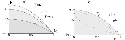
Figure 12: Panel $a)$ contains the region of parameters $(a,c)$ allowed by relation (242) and describing the one–qubit Davies maps. The upper border lines are also drawn for different temperature $T$. Panel $b)$ shows the region allowed for a given temperature $T$. The lines describe two semigroup corresponding to two different randomly chosen generators $\mathcal{L}_{1}$ and $\mathcal{L}_{2}$. The extremal lines corresponding to the solid line on panel $a$ describe the semigroup with the smallest ratio of decoherence to the damping rate. Maps $\operatorname{id},\Phi_{0},\Phi_{CG}$ are the identity channel, completely depolarizing and coarse graining channel respectively.

One–qubit Davies map can be written using the Bloch parametrization (42)

$$\Phi=\bordermatrix{&{}\cr&1&0&0&0\cr&0&\eta_{1}&0&0\cr&0&0&\eta_{1}&0\cr&\kappa_{3}&0&0&\eta_{3}\cr}.$$ (244)

where $|\eta_{i}|$ denote the lengths of axes of the ellipsoid and $\vec{\kappa}$ is the translation vector. These parameters are related to the parameters $(a,c,p)$

$$\eta_{1}=c\geq 0,\qquad\eta_{3}=1-\frac{a}{1-p}\geq 0,$$

$$\kappa_{1}=\kappa_{2}=0,\qquad\kappa_{3}=a\frac{2p-1}{1-p}\geq 0.$$ (245)

The image of the set of pure states under an action of one–qubit Davies map is shown in Fig. 13. The image of the Bloch ball forms an ellipsoid with rotational symmetry. Fig. 13 presents the image of an exemplary one–qubit Davies map for which $\eta_{1}\geq\eta_{3}$, however conditions (242) admits also the case $\eta_{3}\geq\eta_{1}$.

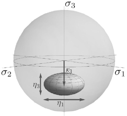
Figure 13: Ellipsoid obtained by an action of a one–qubit Davies channel on the Bloch sphere. The channel is characterized by parameters $(\eta_{1},\eta_{3},\kappa_{3})$ defined in (245).

5.4 Physical examples

Qubit maps of the structure similar to (244) were analysed before in context of quantum optics. The unitary evolution is induced by the laser field, while the dissipative dynamics is caused by an interaction with the environment. The state of a two level atom is characterized by the Bloch vector $(x,y,z)$, where $z$ represents the difference between the diagonal entries of a density matrix equal to the inversion of populations of the atomic levels. Variables $x$ and $y$ are associated with the atomic dipole operators. The evolution in this set has been defined by means of variables describing the decay rate $\tau_{1}$ of the coherences and the rate $\tau_{2}$ of attaining the equilibrium state. These parameters correspond to the variables considered in the Section 5.3, $\eta_{1}=\exp{(-t/\tau_{1})}$ and $\eta_{3}=\exp{(-t/\tau_{3})}$ which are related to squeezing of the axes of the ellipsoid. Formula (242) corresponds to the relation between the decay rates:

$$\tau_{1}\leq 2\tau_{3}.$$ (246)

This relation was obtained by analysing a concrete physical model of the evolution of the two level system by means of Bloch equations [97]. The one–qubit operations (244) were also studied by [98].

5.5 Minimal output entropy of Davies maps

In context of transmission of quantum information, it is natural to ask, which pure states are the most resistant with respect to the changes caused by the Davies maps. The answer depends on the selected measure of decoherence. Such a measure can be described, for example, by means of some matrix norm of the output state maximized over the input states. Among quantities measuring the decoherence, the minimal output entropy is of special importance because some questions concerning the channel capacity, such as additivity problem, can be related with similar problem written in terms of minimal output entropy. The minimal output entropy is related to the maximal norm of the output state if the input is pure.

Since a Davies map has rotational symmetry, the minimizer can be chosen to be a real state:

$$\rho=\begin{pmatrix}\mu&\nu\\ \nu&1-\mu\end{pmatrix},$$ (247)

where $\nu^{2}=(1-\mu)\mu$ since the state is pure. After an action of the operation (240) this state is transformed into

$$\rho^{\prime}=\begin{pmatrix}(1-a)\mu+b(1-\mu)&c\nu\\ c\nu&a\mu+(1-b)(1-\mu)\end{pmatrix},$$ (248)

where $b=ap/(1-p)$. Computing the eigenvalues and minimizing the entropy over $\mu$ one can characterize the minimizer in two cases:

• If $c^{2}\leq(1-a-b)(1-2b)$ the minimizer is characterized by $\mu=0$ and it forms an eigenstate of the Hamiltonian $H$.

• If $c^{2}\geq(1-a-b)(1-2b)$ the minimizer is characterized by

  $$\mu=\frac{(a+b-1)(2b-1)-c^{2}}{2(a+b-1)^{2}-2c^{2}}.$$ (249)

  It is no longer the eigenvalue of the Hamiltonian, however, after some time of the evolution $t\gg 0$ the second case changes into the first one and the minimizer is a state ${\rm diag}(0,1)$. This is an eigenstate of the Hamiltonian. The situation that the minimizer is in the vector ${\rm diag}(0,1)$ reminds the classical evolution of two–dimensional vector governed by the stochastic matrix. In this case the extremal vector like $(0,1)$ is the minimizer of the Shannon entropy of the output.

5.6 Multiplicativity of maximal output norm of one–qubit Davies maps

As discussed in the introduction to Chapter 4, the question of additivity of minimal output von Neumann entropy with respect to the tensor product of quantum operations is one of the most interesting problem in quantum information theory. This problem can be equivalently stated in terms of channel capacity. In general, the conjecture on additivity of channel capacity is false, however, there is still an interesting problem, for which class of maps the conjecture can be confirmed.

Recent studies of the problem use the notion of the Rényi entropy of order $q$. This entropy tends to the von Neumann version as $q\rightarrow 1$. The problem of additivity of minimal output Rényi $q$ entropy is directly related to multiplicativity of the maximal output Schatten $q$–norm. This norm is defined as

$$\|X\|^{S}_{q}=(\operatorname*{Tr}|X|^{q})^{1/q},$$ (250)

where $|X|=\sqrt{X^{\dagger}X}$. Maximal Schatten $q$ norm of a quantum map $\Phi$ is:

$$\|\Phi\|^{S}_{q}:=\max_{\rho}(\operatorname*{Tr}|\Phi(\rho)|^{q})^{1/q},$$ (251)

where maximization is taken over the entire set of density matrices $\rho$. The Rényi entropy of order $q$ of a state $\rho$ can be defined as follows [107]

$$S_{q}(\rho)=\frac{q}{1-q}\log\|\rho\|^{S}_{q}.$$ (252)

Due to logarithm in this formula the multiplicativity of maximal $q$–norm is equivalent to the additivity of minimal output entropy $S^{\min}_{q}$.

In this section, multiplicativity of operator 2–norm induced by the Euclidean vector norm will be proved for the quantum one–qubit Davies maps. This vector induced norm is not related to the Rényi entropy by such an elegant formula like it is in the case for Schatten norm, however, it is a bit easier to calculate than the Schatten counterpart. These particular results support the general solution for multiplicativity problem for Schatten 2–norm which implies the additivity property for minimal output Rényi entropy of order 2 and which has been already proved for general one–qubit quantum operations [99] (see also [18]).

5.6.1 Outline of the proof of multiplicativity

The Euclidean norm (2–norm) of a vector $x=(x_{1},...,x_{n})$ is defined as:

$$\left\|x\right\|_{2}=\sqrt{\sum_{i=1}^{n}\ \left|x_{i}\right|^{2}}.$$ (253)

This vector norm induces the 2–norm of an operator $A$:

$$\left\|A\right\|_{2}={\rm max}_{x\neq 0}\frac{\left\|Ax\right\|_{2}}{\left\|x\right\|_{2}}.$$ (254)

One of the property of this norm (see [100]) is that $\|A\|_{2}$ is equal to square root of the spectral radius of $A^{\dagger}A$ or equivalently to the greatest singular value of the matrix $A$,

$$\left\|A\right\|_{2}=\left[r(A^{\dagger}A)\right]^{1/2},$$ (255)

where a spectral radius $r(A^{\dagger}A)={\rm max}_{i}\left|\xi_{i}\right|$ and $\xi_{i}$ are eigenvalues of $A^{\dagger}A$. In this section the maximal two norm of the output of a quantum map $\Phi:\mathcal{M}_{N}\rightarrow\mathcal{M}_{N}$ will be considered

$$M_{\Phi}=\max_{\rho\in\mathcal{M}_{N}}\|\Phi(\rho)\|_{2}=\max_{A\geq 0}\frac{\|\Phi(A)\|_{2}}{\operatorname*{Tr}A}.$$ (256)

One can ask, whether the maximal two–norm is multiplicative in a sense:

$$M_{\Phi\otimes\Omega}=M_{\Phi}M_{\Omega}.$$ (257)

It will be shown that if $\Phi$ is one–qubit Davies map and $\Omega$ is an arbitrary quantum map acting on $N$–dimensional state the multiplicativity holds.

The idea of the proof of the theorem given below is borrowed from the paper of King and Ruskai [54]. These authors prove an analogical theorem about a bistochastic quantum map $\Phi$. They noted that the same proof holds as well for stochastic one–qubit maps. Here we will present an explicit calculations for the case of Davies maps with $|\eta_{3}|\leq|\eta_{1}|$.

Theorem 8.

Let $\Phi:\mathcal{M}_{2}\rightarrow\mathcal{M}_{2}$ be an one–qubit Davies map and $\Omega:\mathcal{M}_{N}\rightarrow\mathcal{M}_{N}$ be an arbitrary quantum map. The maximal two norm of the output is multiplicative:

$$M_{\Phi\otimes\Omega}=M_{\Phi}M_{\Omega}.$$ (258)

In this section the sketch of the proof will be given, while some details of the calculation will be presented in the next section. In order to present the proof we need to introduce the following set. An arbitrary density matrix on $\mathcal{H}_{2}\otimes\mathcal{H}_{N}$ can be written as a block matrix

$$\rho=\bordermatrix{&{}\cr&\rho_{1}&\gamma\cr&\gamma^{\dagger}&\rho_{2}\cr},$$ (259)

where $\rho_{1},\ \rho_{2},\ \gamma$ are $N\times N$ matrices and the trace condition ${\rm Tr}(\rho_{1}+\rho_{2})=1$ is satisfied. The output state of the product of two quantum operations $\Phi\otimes\Omega$, can be described by:

$$\big{(}\Phi\otimes\Omega\big{)}(\rho)=\bordermatrix{&{}\cr&P&L\cr&L^{\dagger}&Q\cr}.$$ (260)

Here $\Phi$ denotes an one–qubit operation, while the map $\Omega$ acts on $\mathcal{M}_{N}$. Also other block matrices will occur and their positivity will play an important role during the proof. The Schur complement lemma [101] ensures positivity of block matrices, see Lemma 1, Section 3.1.

To demonstrate additivity (258) we shall analyse the inequality $M_{\Phi\otimes\Omega}\geq M_{\Phi}M_{\Omega}$ which is almost immediate since the equality is attained by a product of states which maximize output norm of each map. Because the entire set of states is larger, it contains product and entangled states, the result of maximizing over the entire set can give only a better result. Therefore to prove multiplicativity of maximal output $2$–norm with respect to the tensor product of two maps it is enough to show that

$$z\geq M_{\Phi}M_{\Omega}\Rightarrow z{\rm 1\rule{0.43057pt}{6.54443pt}\hskip 0.86108pt}-\big{(}\Phi\otimes\Omega\big{)}(\rho)\geq 0.$$ (261)

Insert the block matrix form (260) to (261). Due to the Schur complement lemma the right hand side of (261) is positive if and only if

$$L(z{\rm 1\rule{0.43057pt}{6.54443pt}\hskip 0.86108pt}-P)^{-1}L^{\dagger}\leq\ z{\rm 1\rule{0.43057pt}{6.54443pt}\hskip 0.86108pt}-Q.$$ (262)

Notice that this inequality holds if

$$\left\|LL^{\dagger}\right\|_{2}\leq(z-\left\|P\right\|_{2})(z-\left\|Q\right\|_{2}),$$ (263)

since using the general property $P\leq\left\|P\right\|$ one gets:

$$L(z\mathbbm{1}-P)^{-1}L^{\dagger} \leq L(z-\left\|P\right\|_{2})^{-1}L^{\dagger}\ \leq\ \left\|LL^{\dagger}\right\|_{2}(z-\left\|P\right\|_{2})^{-1}$$ (264)

$$\leq (z-\left\|Q\right\|_{2})\ \leq\ z\mathbbm{1}-Q.$$ (265)

Therefore the positivity of $(z-\left\|P\right\|_{2})$ and $(z-\left\|Q\right\|_{2})$ and inequality (263) are the only relations needed to prove Theorem 258. These relations will be proved in the next section for the case of $\Phi$ being an arbitrary one–qubit Davies map with $|\eta_{3}|\leq|\eta_{1}|$.

5.6.2 Details of the proof of multiplicativity

Proof.

of Theorem 258. It is necessary to find the specific form of $M_{\Phi},\ P$ an $Q$ in (260), then to check positivity of $(M_{\Phi}M_{\Omega}-\left\|P\right\|_{2})$ and $(M_{\Phi}M_{\Omega}-\left\|Q\right\|_{2})$, and finally to prove (263). Let us restrict our considerations to the case of Davies maps $\Phi$, for which $\eta_{3}^{2}\leq\eta_{1}^{2}$ in (244) as discussed in Section 5.6.1.

• Maximal 2–norm of the output, $M_{\Phi}$.

  Use the Bloch parametrization of $\Phi$ as in (244), let it act on the Bloch vector $(1,x,y,z)^{\dagger}$, where $x,y,z$ are real. Moreover $x^{2}+y^{2}+z^{2}=1$ guarantees restriction to pure states. It is enough to take pure input state because the 2–norm is convex on the set of density matrices and it attains maximum at the boundary of the set. The spectral radius of the square of the output state reads according to (255):

  $$\sqrt{[r(\Phi(\rho)^{\dagger}\Phi(\rho))]}=\frac{1}{2}\big{(}1+\sqrt{(\kappa_{3}+z\eta_{3})^{2}+(1-z^{2})\eta_{1}^{2}}\big{)}.$$ (266)

  Since the image of the Davies map has rotational symmetry, there are no parameters $x$ and $y$ in this formula. Second derivative of the function (266) with respect to $z$ is negative under the condition: $\eta_{3}^{2}\ \leq\ \eta_{1}^{2}$. Therefore function (266) has a maximum:

  $$M_{\Phi}=\frac{1}{2}\left(1+\sqrt{\eta_{1}^{2}+\frac{\kappa_{3}^{2}\eta_{1}^{2}}{\eta_{1}^{2}-\eta_{3}^{2}}}\right).$$ (267)

• Output of a product map.

  Now the explicit form of matrices $P,\ Q$ and $L$ of the output state (260) will be given. Consider an one–qubit input state. A vector $(1,x,y,z)^{\dagger}$ corresponds to the density matrix:

  $$\rho=\frac{1}{2}\bordermatrix{&{}\cr&1+z&x+iy\cr&x-iy&1-z\cr}.$$ (268)

  Its image with respect to a Davies map (244) reads:

  $$\Phi(\rho)=\frac{1}{2}\bordermatrix{&{}\cr&1+z\eta_{3}+\kappa_{3}&\eta_{1}(x+iy)\cr&\eta_{1}(x-iy)&1-z\eta_{3}-\kappa_{3}\cr}.$$ (269)

  In the analogous way the initial state in a space $\mathcal{M}_{2N}$ can be given by (259)

  $$\rho=\frac{1}{2}\bordermatrix{&{}\cr&\rho_{1}+\rho_{2}+\hat{z}&\hat{x}+i\hat{y}\cr&\hat{x}-i\hat{y}&\rho_{1}+\rho_{2}-\hat{z}\cr},$$ (270)

  where $\hat{z}=\rho_{1}-\rho_{2}$ and $\hat{x}-i\hat{y}=2\gamma$ are $N\times N$ matrices. The output state of a map $\Phi\otimes{\rm 1\rule{0.43057pt}{6.54443pt}\hskip 0.86108pt}$ is: ​​​​​​

  $$\big{(}\Phi\otimes\operatorname{id}\big{)}(\rho)=$$

  $$\bordermatrix{&{}\cr&\frac{1}{2}\big{(}\rho_{1}+\rho_{2}+\eta_{3}(\rho_{1}-\rho_{2})+\kappa_{1}(\rho_{1}+\rho_{2})\big{)}&\eta_{1}\gamma\cr&\eta_{1}\gamma^{\dagger}&\frac{1}{2}\big{(}\rho_{1}+\rho_{2}-\eta_{3}(\rho_{1}-\rho_{2})-\kappa_{3}(\rho_{1}+\rho_{2})\big{)}\cr}.$$

  Finally the matrices $P,Q$ and $L$ are defined by comparison of suitable blocks of two block matrices:

  $$\big{(}\Phi\otimes\Omega\big{)}(\rho)=\bordermatrix{&{}\cr&P&L\cr&L^{\dagger}&Q\cr}$$

  $$= \!\!\!\!\!\!\!\!\!\!\!\bordermatrix{&{}\cr&\frac{1}{2}\Omega\big{(}\rho_{1}+\rho_{2}+\eta_{3}(\rho_{1}-\rho_{2})+\kappa_{3}(\rho_{1}+\rho_{2})\big{)}&\eta_{1}\Omega\big{(}\gamma\big{)}\cr&\eta_{1}\Omega\big{(}\gamma\big{)}^{\dagger}&\frac{1}{2}\Omega\big{(}\rho_{1}+\rho_{2}-\eta_{3}(\rho_{1}-\rho_{2})-\kappa_{3}(\rho_{1}+\rho_{2})\big{)}\cr}.$$

• Multiplicativity.

  One can use the property $\left\|\Omega(\rho)\right\|_{2}\leq{\rm Tr}(\rho)M_{\Omega}$ (256) to show that $(M_{\Phi}M_{\Omega}-\left\|P\right\|_{2})$ is positive. It is so if

  $$\frac{1}{2}M_{\Omega}\Big{(}1+\sqrt{\eta_{1}^{2}+\frac{\kappa_{3}^{2}\eta_{1}^{2}}{\eta_{1}^{2}-\eta_{3}^{2}}}\Big{)}>\frac{1}{2}M_{\Omega}\Big{(}{\rm Tr}(\rho_{1}+\rho_{2})+\eta_{3}(\rho_{1}-\rho_{2})+\kappa_{3}(\rho_{1}+\rho_{2})\Big{)}.$$ (273)

  Notice that ${\rm Tr}(\rho_{1}+\rho_{2})=1$. To show that the above inequality is true, it is sufficient to prove:

  $$\sqrt{\eta_{1}^{2}+\frac{t^{2}\eta_{1}^{2}}{\eta_{1}^{2}-\eta_{3}^{2}}}>\eta_{3}+\kappa_{3}.$$ (274)

  Taking the square of both sides one gets the expression:

  $$\left(\kappa_{3}\eta_{3}-(\eta_{1}^{2}-\eta_{3}^{2})\right)^{2}>0.$$ (275)

  This implies that $(M_{\Phi}M_{\Omega}-\left\|P\right\|_{2})>0$. In a similar way we prove the positivity of $(M_{\Phi}M_{\Omega}-\left\|Q\right\|_{2})$. The last step is to prove inequality (263). Consider a positive block matrix $\big{(}{\rm 1\rule{0.43057pt}{6.54443pt}\hskip 0.86108pt}\otimes\Omega\big{)}(\rho)=\bordermatrix{&{}\cr&\Omega(\rho_{1})&\Omega(\gamma)\cr&\Omega(\gamma^{\dagger})&\Omega(\rho_{2})\cr}$. Assume that $\Omega(\rho_{1})>0$ (if $\Omega(\rho_{1})\geq 0$ one can add $\epsilon{\rm 1\rule{0.43057pt}{6.54443pt}\hskip 0.86108pt}$ to $\rho_{1}$ and eventually take the limit $\epsilon\rightarrow 0$). Due to the inequality $\Omega(\rho_{1})\leq\|\Omega(\rho_{1})\|_{2}$ one can write

  $$\langle v|\Omega(\gamma)\Omega(\gamma)^{\dagger}|v\rangle\leq\|\Omega(\rho_{1})\|_{2}\langle v|\Omega(\gamma)\Omega(\rho_{1})^{-1}\Omega(\gamma)^{\dagger}|v\rangle.$$ (276)

  Due to the Schur complement lemma we have $\Omega(\rho_{2})\geq\Omega(\gamma)\Omega(\rho_{1})^{-1}\Omega(\gamma)^{\dagger}$ and therefore,

  $$\|\Omega(\rho_{1})\|_{2}\langle v|\Omega(\gamma)\Omega(\rho_{1})^{-1}\Omega(\gamma)^{\dagger}|v\rangle\leq\|\Omega(\rho_{1})\|_{2}\langle v|\Omega(\rho_{2})|v\rangle\leq\|\Omega(\rho_{1})\|_{2}\|\Omega(\rho_{2})\|_{2}.$$ (277)

  Hence the inequality $\|\Omega(\gamma)\Omega(\gamma)^{\dagger}\|_{2}\leq\|\Omega(\rho_{1})\|_{2}\|\Omega(\rho_{2})\|_{2}$ holds. This inequality together with definition (256) implies

  $$\|\Omega(\gamma)\Omega(\gamma)^{\dagger}\|_{2}\leq M_{\Omega}^{2}\operatorname*{Tr}\rho_{1}\operatorname*{Tr}\rho_{2}.$$ (278)

  Denote ${\rm Tr}(\rho_{1})$ by $x$. To prove inequality (263) it is enough to show that the second inequality holds in the expression below

  $$\left\|LL^{\dagger}\right\|_{2}=\eta_{1}^{2}\left\|\Omega(\gamma)\right\|_{2}^{2}\leq\eta_{1}^{2}x(1-x)M_{\Omega}^{2}\leq(M_{\Phi}M_{\Omega}-\left\|P\right\|_{2})(M_{\Phi}M_{\Omega}-\left\|Q\right\|_{2}),$$ (279)

  and this is true if

  $$\eta_{1}^{2}x(1-x)M_{\Omega}^{2}\leq\frac{1}{4}M_{\Omega}^{2}\Big{[}\eta_{1}^{2}+\frac{\kappa_{3}^{2}\eta_{1}^{2}}{\eta_{1}^{2}-\eta_{3}^{2}}-(\eta_{3}(2x-1)+\kappa_{3})^{2}\Big{]}.$$ (280)

  This inequality can be shown by taking the function which is the difference between the right hand side and the left hand side. The second derivative of this function is equal to $2(\eta_{1}^{2}-\eta_{3}^{2})$. Therefore whenever $(\eta_{1}^{2}>\eta_{3}^{2})$ the difference is a convex function which has minimum at $0$. That finishes the proof of the last inequality. Therefore inequality (263) holds and it proves Theorem 258.

∎

In the case $|\eta_{1}|\leq|\eta_{3}|$ the proof goes analogously. The maximal output norm (267) has in this case a simpler form, since the maximizer is a pure state described by the Bloch vector $(x=0,y=0,z=1)$. The specific form of the Davies map was used in this proof in (267) when the formula of the maximal output norm was computed and in formula (• ‣ 5.6.2). Moreover, positivity of $\kappa_{3}$ is used in (274).

5.7 Davies maps acting on qutrits

In this chapter a characterization of the Davies maps for qutrits, $N=3$, will be given. Going to higher dimensions demands more abstract and systematic approach than in the case of one–qubit maps. The entire evolution consists of the unitary part and the dissipative part and such is the structure of the generator $\mathcal{G}=i\delta+\mathcal{L}$. The unitary evolution $\delta$ is governed by the Hamiltonian which in its eigenbasis has a form $H=\sum_{i=1}^{3}\epsilon_{i}|i\rangle\langle i|$, where $\epsilon_{1}>\epsilon_{2}>\epsilon_{3}$. Differences of energies $\{\omega_{ij}=\epsilon_{i}-\epsilon_{j}\}$ are called Bohr frequencies. They are eigenvalues of the unitary part of the evolution, $\delta$ given by $\rho\rightarrow[H,\rho]$, while the eigenvectors of $\delta$ are $|i\rangle\langle j|$ for $i,j=1,2,3$. Assume that the set of Bohr frequencies is not degenerated beside the zero frequency case, $\omega_{ii}$. The subspace related to the zero frequency is $3$–dimensional. Since the dissipative part $\mathcal{L}$ of the evolution commutes with the unitary part, it has the same eigenvectors and therefore it does not couple the non-degenerated subspaces. Thus the off diagonal entries of a density matrix are not mixed with the diagonal ones, if the matrix is written in the eigenbasis of the Hamiltonian.

Like in the case of one–qubit maps only the dissipative part of the evolution will be analysed. An one–qutrit Davies map has a structure

$$\Phi=\bordermatrix{&{}\cr&1-\mathcal{F}_{21}-\mathcal{F}_{31}&0&0&0&\mathcal{F}_{12}&0&0&0&\mathcal{F}_{13}\cr&0&\mu_{1}&0&0&0&0&0&0&0\cr&0&0&\mu_{2}&0&0&0&0&0&0\cr&0&0&0&\mu_{1}&0&0&0&0&0\cr&\mathcal{F}_{21}&0&0&0&1-\mathcal{F}_{12}-\mathcal{F}_{32}&0&0&0&\mathcal{F}_{23}\cr&0&0&0&0&0&\mu_{3}&0&0&0\cr&0&0&0&0&0&0&\mu_{2}&0&0\cr&0&0&0&0&0&0&0&\mu_{3}&0\cr&\mathcal{F}_{31}&0&0&0&\mathcal{F}_{32}&0&0&0&1-\mathcal{F}_{13}-\mathcal{F}_{23}\cr},$$ (281)

where $\mathcal{F}_{21},\mathcal{F}_{31},\mathcal{F}_{32}$ and $\mu_{1},\mu_{2},\mu_{3}$ parametrize the map. The off–diagonal elements are related by the detailed balance formula

$$\mathcal{F}_{ij}p_{j}=\mathcal{F}_{ji}p_{i}.$$ (282)

Here $p_{i}$ determine the invariant Gibbs state (236). The Choi-Jamiołkowski matrix of (281) preserves the same structure:

$$D_{\Phi}=\frac{1}{3}\bordermatrix{&{}\cr&1-\mathcal{F}_{31}-\mathcal{F}_{21}&0&0&0&\mu_{1}&0&0&0&\mu_{2}\cr&0&\mathcal{F}_{12}&0&0&0&0&0&0&0\cr&0&0&\mathcal{F}_{13}&0&0&0&0&0&0\cr&0&0&0&\mathcal{F}_{21}&0&0&0&0&0\cr&\mu_{1}&0&0&0&1-\mathcal{F}_{32}-\mathcal{F}_{21}&0&0&0&\mu_{3}\cr&0&0&0&0&0&\mathcal{F}_{23}&0&0&0\cr&0&0&0&0&0&0&\mathcal{F}_{31}&0&0\cr&0&0&0&0&0&0&0&\mathcal{F}_{32}&0\cr&\mu_{2}&0&0&0&\mu_{3}&0&0&0&1-\mathcal{F}_{32}-\mathcal{F}_{31}\cr}.$$ (283)

The generator and its Choi-Jamiołkowski matrix have also the same structure.

Block of the superoperator $\Phi$ of the Davies quantum operation which is related to zero frequency space is a $3\times 3$ stochastic matrix

$$\mathcal{F}=\bordermatrix{&{}\cr&1-\mathcal{F}_{31}-\mathcal{F}_{21}&\mathcal{F}_{12}&\mathcal{F}_{13}\cr&\mathcal{F}_{21}&1-\mathcal{F}_{21}-\mathcal{F}_{32}&\mathcal{F}_{23}\cr&\mathcal{F}_{31}&\mathcal{F}_{32}&1-\mathcal{F}_{13}-\mathcal{F}_{23}\cr},$$ (284)

where $\mathcal{F}_{32},\mathcal{F}_{31},\mathcal{F}_{21}\geq 0.$ Due to the definition of the quantum detailed balance condition (237) the Davies map is Hermitian with respect to scalar product $\langle X,Y\rangle_{\beta}:=\operatorname*{Tr}\rho_{\beta}^{-1}X^{\dagger}Y$ and therefore it has a real spectrum. Moreover, the spectrum is positive, since there is real logarithm of the matrix $\Phi$ represented the Davies map. The positivity of the zero frequency block implies that

$$\begin{array}[]{c}\mathcal{F}_{32}+\mathcal{F}_{31}+\mathcal{F}_{21}\leq 1,\\ 3-4(\mathcal{F}_{32}+\mathcal{F}_{31}+\mathcal{F}_{21})+3(\mathcal{F}_{32}\mathcal{F}_{31}+\mathcal{F}_{31}\mathcal{F}_{21}+\mathcal{F}_{21}\mathcal{F}_{32})\geq 0.\end{array}$$ (285)

The question considered in this chapter concerns explicit analytical relations for entries of the superoperator (281), which imply that the superoperator represents a Davies map. One of the condition for $\Phi$ is that there exists an exponential form

$$\mathcal{F}=e^{Lt}.$$ (286)

Operator $L$ is the zero frequency part of the contractive part of the generator of completely positive Davis semigroup. It is parameterized as follows:

$$L=\bordermatrix{&{}\cr&-L_{21}-L_{31}&L_{12}&L_{13}\cr&L_{21}&-L_{12}-L_{32}&L_{23}\cr&L_{31}&L_{32}&-L_{13}-L_{23}\cr}.$$ (287)

This is only the zero frequency block which satisfies the detailed balance condition. The entire dissipative part of the generator is represented by a $9\times 9$ matrix. Its Choi matrix has on diagonal elements $L_{32},L_{31},L_{21}$. Since the Choi state of the generator has to be positive on the subspace perpendicular to the maximally entangled state we need to require that $L_{32},L_{31},L_{21}\geq 0$.

In the next section an explicit calculation of the logarithm of a stochastic matrix of order three (284) is presented.

5.7.1 Logarithm of a stochastic matrix of size three

To compute analytically the logarithm of a positive matrix (284) one may relay on the following construction. As matrix $\mathcal{F}$ has the eigenvalues $\left\{1,x+y,x-y\right\}$, where

$$\begin{array}[]{l}x=\frac{1}{2}(\operatorname*{Tr}\mathcal{F}-1),\\ y=\frac{1}{2}\sqrt{2\operatorname*{Tr}\mathcal{F}^{2}-(\operatorname*{Tr}\mathcal{F})^{2}+2\operatorname*{Tr}\mathcal{F}-3},\end{array}$$ (288)

the logarithm has the form

$$\log(\mathcal{F})=\log\Big{[}U\bordermatrix{&{}\cr&1&0&0\cr&0&x+y&0\cr&0&0&x-y\cr}U^{-1}\Big{]},$$ (289)

where $U$ is a unitary matrix which transforms $\mathcal{F}$ into its diagonal form. Let us evaluate $\log(\mathcal{F})$ without computing the matrix $U$ explicitly. One can write that

$$\log(\mathcal{F})=\frac{1}{2}\Big{[}\log(x^{2}-y^{2})Z^{2}+\log(\frac{x+y}{x-y})Z\Big{]},$$ (290)

where

$$Z=U\bordermatrix{&{}\cr&0&0&0\cr&0&1&0\cr&0&0&-1\cr}U^{-1}.$$ (291)

The matrix $\mathcal{F}$ can be given in terms of $Z$:

$$\mathcal{F}=1-Z^{2}+xZ^{2}+yZ.$$ (292)

This relation allows one to compute $yZ=(\mathcal{F}-1)-(x-1)Z^{2}.$ Formula for $Z^{2}$ can be calculated by taking the square of this equation and using the fact that $Z^{4}=Z^{2}$ and that $Z^{2}(\mathcal{F}-1)=(\mathcal{F}-1)Z^{2}=(\mathcal{F}-1)$. The last formula holds since operator $(\mathcal{F}-1)$ is defined in the subspace for which $Z^{2}$ is the identity,

$$Z^{2}=\frac{(\mathcal{F}-1)\left[(\mathcal{F}-1)-2(x-1)\right]}{y^{2}-(x-1)^{2}}.$$ (293)

Therefore the logarithm of the matrix $\mathcal{F}$ can be expressed according to Eq. (290). By comparing a suitable entries of $\log(\mathcal{F})$ with the parameters of $L$, one gets the parameter $L_{21}$ as a function of $(\mathcal{F}_{32},\mathcal{F}_{31},\mathcal{F}_{21})$,

$$L_{21}=y_{2}(1-x-y)\log(x-y)-(y_{1}(1-x+y)\log(x+y)),$$ (294)

where $x$ and $y$ are given by Eq. (288) and

$$y_{1} := 2y-\mathcal{F}_{12}-\mathcal{F}_{21}+\mathcal{F}_{13}-\mathcal{F}_{31}+\mathcal{F}_{23}-\mathcal{F}_{32}+2\frac{\mathcal{F}_{23}\mathcal{F}_{31}}{\mathcal{F}_{21}},$$ (295)

$$y_{2} := 4-2y-\mathcal{F}_{12}-\mathcal{F}_{21}+\mathcal{F}_{13}-\mathcal{F}_{31}+\mathcal{F}_{23}-\mathcal{F}_{32}+2\frac{\mathcal{F}_{23}\mathcal{F}_{31}}{\mathcal{F}_{21}}.$$ (296)

The set of points $\left\{\mathcal{F}_{23},\mathcal{F}_{13},\mathcal{F}_{12}\right\}$, which defines the set of symmetric bistochastic matrices from the dynamical semigroup, is shown in Fig. 14 and Fig. 15 denoted by $\mathsf{E}$. This set is inside the set of all bistochastic $3\times 3$ matrices which is denoted by $\mathsf{D}$. The boundaries of the set are stated by the constraints $L_{21},L_{31},L_{32}\geq 0$.

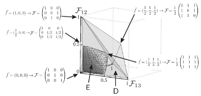
Figure 14: The set $\mathsf{E}$ of $3\times 3$ bistochastic matrices $\mathcal{F}$ (284), which form the zero frequency block of the Davies channel $\Phi$ (281) under condition $T\rightarrow\infty$, is represented by the vector of the off–diagonal elements $\vec{f}=\{\mathcal{F}_{12},\mathcal{F}_{13},\mathcal{F}_{23}\}$. The set $\mathsf{E}$ is inside the set of all bistochastic $3\times 3$ matrices $\mathsf{D}$. The characteristic points are denoted by $\vec{f}$ and the corresponding matrix $\mathcal{F}$.

Expression (294) allows one to check that the set of stochastic matrices belonging to the semigroup of completely positive maps with the detailed balance condition is not convex. Consider two exemplary points which lie near the border of the cross-section and belong to the set ($L_{21}\geq 0$): $\left\{0.5,0,0\right\}$ and $\left\{0.22744,0.22744,0.04512\right\}$. Their convex combination does not belong to the set. Therefore the set of Davies map is not convex. Fig. 15 presents the cross-section of the set of bistochastic matrices which form the zero frequency part of the Davies map represented in the space of parameters $\mathcal{F}_{21},\mathcal{F}_{31},\mathcal{F}_{32}$. Fig. 15b plots a non–convex cross–section of the set $\mathsf{E}$ by the plane $\mathsf{M}$.

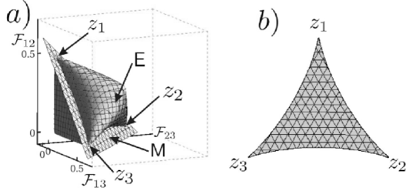
Figure 15: $a)$ The set $\mathsf{E}$ of $3\times 3$ bistochastic matrices $\mathcal{F}$ (284), which form the zero frequency block of the Davies channel $\Phi$ (281) under condition $T\rightarrow\infty$, is represented by the vector of the off–diagonal elements $\{\mathcal{F}_{12},\mathcal{F}_{13},\mathcal{F}_{23}\}$. The set $\mathsf{E}$ is cut by the plane $\mathsf{M}:\mathcal{F}_{12}+\mathcal{F}_{13}+\mathcal{F}_{23}=\frac{1}{2}$. The cross–section is presented in Panel $b)$ and shows that the set $\mathsf{M}$ is not convex.

In order to obtain a full characterization of the Davies map for qutrits, not only its zero frequency par have to be analysed. One needs to take into consideration also the complete positivity condition and the condition on the semigroup related to the Choi–Jamiołkowski matrices of the superoperator and its generator. These conditions allow us to specify the matrix entries $\mu_{i}$ from Eq. (281).

In this way the full characterization of the Davies channels for one–qubit and one–qutrits is provided.

6 Concluding remarks and open problems

The aim of this thesis was to investigate quantum channels on different levels of generality and using different approaches. For instance, general properties of quantum channels were considered in Chapter 2, while some particular classes of one–qubit and one–qutrit quantum channels were analysed in Part III of these thesis. The Davies maps motivated by a specific physical model were studied in Chapter 5. Some useful characteristics of a quantum channel are provided by different kinds of entropies. Among them we used the minimal output entropy, the entropy of a map, the entropy of an environment which takes part in an evolution described by a channel. Apart of the standard von Neumann entropy which is the quantum counterpart of the Shannon entropy, the quantum Rényi and Tsallis entropies were also applied.

In Part II the universal entropic inequality for an arbitrary ensemble of quantum states is proved for the von Neumann entropy. This part of the thesis treats a quantum channel as a device preparing a quantum ensemble. The Holevo quantity of this ensemble is shown to be bounded by the entropy of an environment, used in the preparation process. The state of the environment after a quantum operation $\Phi$ is equivalent to the output of the complementary channel $\tilde{\Phi}$.

One can define selfcomplementary channels for which $\Phi(\rho)=\tilde{\Phi}(\rho)$ for any $\rho$. Relation (38) between the Kraus operators of $\Phi$ and the Kraus operators of $\tilde{\Phi}$ is useful to specify selfcomplementary channels. Since the coherent information (102) of such channels is equal to $0$, the same holds also for the quantum channel capacity (103). Identification of selfcomplementary channels, as well as investigation of their properties are worth to be studied in future.

Chapter 3 contains the conjecture which establishes a relation between the Holevo quantity, and the matrix of fidelities. This leads to a geometric characterization of the states in the ensemble. The bound on the Holevo quantity proved in Chapter 2 can be also related to other notions of quantum information theory, such as the quantum discord [102], [103] which measures the quantum correlations in a two–partite system.

The study of quantum channels is an important task of the modern theory of quantum information. For example, the problem of additivity of the channel capacity, or equivalently, additivity of the minimal output entropy remains open even for channels acting on a single qubit. Results presented in this thesis could be further developed to investigate the additivity conjecture for different classes of quantum channels.

Some results of Chapter 4 concern general properties of quantum channels. For instance we proved the additivity of the map entropy (214), and Theorem 6 establishing the extremal position of depolarizing channels in the set of all channels characterized by the Rényi entropies $S_{2}^{\min}(\Phi)$ and $S_{2}^{\operatorname*{map}}(\Phi)$. These results allow us to pose Conjecture 2 specifying pairs of maps for which the additivity of channel capacity may hold.

In Part III, some specific types of channels are investigated. Properties of one–qubit channels are analysed in Chapter 4. Some transformations on one–qubit quantum channels defined in Section 4.3 lead to new results on the characterization of the set of quantum channels in the plane $(S^{\min}(\Phi),S^{\operatorname*{map}}(\Phi))$. The aim of this analysis is to find some conditions that enable one to estimate the minimal output entropy, which is difficult to compute, by the entropy of the map easy to calculate.

The Davies channels, which correspond to a concrete physical model, are studied in Chapter 5. Superoperators of the Davies maps are specified in the case of one–qubit maps and one–qutrit maps. The question whether the channel capacity of the Davies maps is additive is still open, although, Davies maps acting on $N$–level system compose the set of only $d=N^{2}-1$ dimensions, while the set of all quantum operations acting on system of the same $N$ has $N^{2}(N^{2}-1)$ dimensions.

The quantum information theory is a modern field of science which creates an environment for new future applications and opens new paths for development of technology. Quantum channels, which describe any possible evolution of a quantum state, play an important role in possible applications. Quantum channels describe decoherence caused by the interaction with an environment. Knowledge of their properties allows one to choose the most efficient quantum protocols for a given purpose. Theoretical investigations uncover new possibilities, new laws and fundamental restrictions on processing of quantum information.

The classical theory of information began with investigations on communication in a given language through given technological tools. However, very fast, the laws of information became treated as fundamental properties of nature. Therefore, studies in the field of quantum information are so exciting.

Appendix 1

In Appendix we analyze ensembles of three one–qubit states $\{\rho_{1}=|\phi_{1}\rangle\langle\phi_{1}|,\rho_{2}=|\phi_{2}\rangle\langle\phi_{2}|,\rho_{3}\}$ and provide calculations related to Fig. 4 necessary to prove Lemma 4 in Section 3.2.

The Bloch vector characterizing the average states can be given by

$$\vec{OA}=a(0,0,1).$$ (297)

The Bloch vector representing the mixed state $\rho_{3}$ is parameterized by an angle $\alpha$

$$\vec{OB}=b(0,\sin{\alpha},\cos{\alpha}).$$ (298)

The vector $\vec{OC}$ is chosen in such a way that the ratio $|CA|:|AB|$ is $1:2$. Therefore one has

$$\vec{OC}=\frac{1}{2}(3\vec{OA}-\vec{OB}).$$ (299)

The point $C$ is in the center of the interval $DE$, between two pure states $|\phi_{1}\rangle$ and $|\phi_{2}\rangle$ characterized by the points $D$ and $E$. Both vectors $\vec{OD}$ and $\vec{OE}$ form with vector $\vec{OC}$ the angle $\gamma$ so that

$$\cos{\gamma}=|OC|.$$ (300)

This is in turn the square root of the fidelity $|\langle\phi_{1}|\phi_{2}\rangle|^{2}$, because the angle $\gamma$ is half of the angle between two pure states,

$$F_{23}=\cos^{2}{\gamma}.$$ (301)

The fidelity between two one–qubit states represented by Bloch vectors $\vec{x}$ and $\vec{y}$ reads

$$F=\frac{1}{2}(1+\vec{x}\cdot\vec{y}).$$ (302)

The scalar product of $\vec{OB}$ and $\vec{OD}$ is equal to:

$$\vec{OB}\cdot\vec{OD}=b\cos{(\mu+\gamma-\gamma)}=b\Big{[}\cos{(\mu+\gamma)}\cos{\gamma}+\sin{(\mu+\gamma)}\sin{\gamma}\Big{]}.$$ (303)

Hence

$$F_{12}=\frac{1}{2}(1+\vec{OC}\cdot\vec{OB}+b\sqrt{1-\frac{(\vec{OC}\cdot\vec{OB})^{2}}{b^{2}\vec{OC}\cdot\vec{OC}}}\sqrt{1-\vec{OC}\cdot\vec{OC}}).$$ (304)

The third fidelity $F_{13}$ can by obtained using Lemma 2. For $\beta=0$ the product of three fidelities used in Lemma 4 is a function $f_{0}(a,b,\alpha,\beta=0)$ given by

$$f_{0}(a,b,\alpha,\beta=0)=F_{12}F_{13}F_{23}=$$ (305)

$$\frac{1}{64}\left(9a^{2}-6b\cos\alpha a+b^{2}\right)\left(b^{2}-3a\cos\alpha b-2\right)^{2}$$ (306)

$$+\frac{1}{64}\left(9a^{2}b^{2}\left(9a^{2}-6b\cos\alpha a+b^{2}-4\right)\sin^{2}\alpha\right).$$ (307)

Appendix 2

In this appendix we present computations necessary to prove Lemma 3. It is convenient to change the basis such that the vector $\vec{OB}$ (see Fig. 4) is transformed into

$$\vec{OB}^{\prime}=b(0,0,1).$$ (308)

Denote the angle $\nu:=\mu+\gamma$, where $\mu$ is the angle between $\vec{OB}$ and $\vec{OD}$. The vectors $\vec{OD}$ and $\vec{OE}$ in the new basis can be obtained by rotating the state $(0,0,1)$ around the axis $x$ by angles:

$$\vec{OD}^{\prime} = U_{x}(\mu)(0,0,1),$$ (309)

$$\vec{OE}^{\prime} = U_{x}(\mu+2\gamma)(0,0,1).$$ (310)

The vectors $\vec{OG}^{\prime}$ and $\vec{OF}^{\prime}$ are obtained by rotating the above vectors around the axis $U_{x}(\nu)(0,0,1)$ by angle $\beta$. Such a rotation can be defined as an action of a unitary matrix $U$ on vectors (309). The unitary matrix is given by

$$U=U_{z}(-\frac{\pi}{2})\,U_{y}(\nu)\,U_{z}(\beta)\,U^{\dagger}_{y}(\nu)\,U^{\dagger}_{z}(-\frac{\pi}{2}),$$ (311)

where the rotation matrices read

$$U_{x}(\alpha)=\begin{pmatrix}1&0&0\\ 0&\cos{\alpha}&-\sin{\alpha}\\ 0&\sin{\alpha}&\cos{\alpha}\end{pmatrix},\quad U_{y}(\alpha)=\begin{pmatrix}\cos{\alpha}&0&\sin{\alpha}\\ 0&1&0\\ -\sin{\alpha}&0&\cos{\alpha}\end{pmatrix},$$

$$U_{z}(\alpha)=\begin{pmatrix}\cos{\alpha}&-\sin{\alpha}&0\\ \sin{\alpha}&\cos{\alpha}&0\\ 0&0&1\end{pmatrix}.$$

One can use formula (302) to calculate the product of three fidelities for three considered states, $\vec{OB}^{\prime},\vec{OG}^{\prime}$ and $\vec{OF}^{\prime}$ as a function of the angle $\beta$.

$$f = F_{12}F_{13}F_{23}$$

$$= \!\!\!\!\!\!\frac{1}{16}\cos^{2}\gamma\left((\cos\mu+\cos(2\gamma+\mu)+2)^{2}-\cos^{2}\beta(\cos\mu-\cos(2\gamma+\mu))^{2}\right).$$

The product of three pairwise fidelities attains its minimum at $\beta=0$ as stated in Lemma 3.

References

- [1] C. Shannon, A Mathematical Theory of Communication, The Bell System Technical Journal, 27 379–423, 623–656 (1948).
- [2] A. Rényi, On measures of information and entropy, Proceedings of the 4th Berkeley Symposium on Mathematics, Statistics and Probability, 547–561 (1960).
- [3] C. Tsallis, Possible generalization of Boltzmann-Gibbs statistics, J. Stat. Phys., 52 479-487 (1988).
- [4] A. Plastino, A. R. Plastino, Tsallis Entropy and Jaynes’ Information Theory Formalism, Brazilian Journal of Physics, 29 50-60 (1999).
- [5] E. Davies, Quantum stochastic processes, Commun. Math. Phys., 15 277–306 (1970).
- [6] A. Kossakowski, On quantum statistical mechanics of non-Hamiltonian systems, Rep. Math. Phys., 3 247–274 (1972).
- [7] A. Holevo, Bounds for the quantity of information transmitted by a quantum communication channel, Prob. Inf. Transm. 9 177–83 (1973).
- [8] M. Nielsen, I. Chuang, Quantum Computation and Quantum Information, Cambridge University Press, Cambridge (2000).
- [9] C.H. Bennett, G. Brassard, C. Crépeau, R. Jozsa, A. Peres, and W.K. Wootters, Teleporting an unknown quantum state via dual classical and Einstein-Podolsky-Rosen channels, Phys. Rev. Lett., 70 1895–1899 (1993).
- [10] D. Deutsch, R. Jozsa, Rapid solutions of problems by quantum computation, Proceedings of the Royal Society of London A, 439 553–558 (1992).
- [11] Grover L.K. A fast quantum mechanical algorithm for database search, Proceedings, 28th Annual ACM Symposium on the Theory of Computing, 212–219 (1996).
- [12] P. Shor, Polynomial-Time Algorithms for Prime Factorization and Discrete Logarithms on a Quantum Computer, SIAM J.Sci.Statist.Comput., 26 1484–1509 (1997).
- [13] M. Horodecki, P. Horodecki, and R. Horodecki, General teleportation channel, singlet fraction, and quasidistillation, Phys. Rev. A, 60 1888–1898 (1999).
- [14] R. Horodecki, P. Horodecki, M. Horodecki, K. Horodecki, Quantum entanglement, Rev. Mod. Phys., 81 865–942 (2009).
- [15] I. Bengtsson and K. Życzkowski, Geometry of Quantum States: An Introduction to Quantum Entanglement, Cambridge University Press, Cambridge (2006)
- [16] M. Hastings, Superadditivity of communication capacity using entangled inputs, Nature Physics, 5 255–257 (2009).
- [17] M. Horodecki, On Hastings counterexamples to the minimum output entropy additivity conjecture, Open Systems Information Dynamics, 17 31–52 (2010) .
- [18] C. King, Remarks on the Additivity Conjectures for Quantum Channels, in: Entropy and the Quantum, eds. R. Sims, D. Ueltschi, Contemporary Mathematics, 529 177–188, University of Arizona (2010).
- [19] C. Bennett, G. Brassard, Quantum Cryptography: Public Key Distribution and Coin Tossing, Proceedings of IEEE International Conference on Computers Systems and Signal Processing, Bangalore India, 175–179 (1984).
- [20] A. Wehrl, General properties of entropy, Rev. Mod. Phys., 50 221–260 (1978).
- [21] M. B. Ruskai, Inequalities for Quantum Entropy: A Review with Conditions for Equality, J. Math. Phys., 43 4358–4375 (2002).
- [22] F. Nielsen, R. Nock, On Rényi and Tsallis entropies and divergences for exponential families, arXiv:1105.3259, (2011).
- [23] C. Shannon, Communication in the presence of noise, Proc. Institute of Radio Engineers, 37 10–21. (1949).
- [24] R. Hartley, Transmission of Information, Bell System Technical Journal, 7 535–563 (1928).
- [25] B. Schumacher, Quantum coding, Phys. Rev. A, 51 2738–2747 (1995).
- [26] E. Desurvire, Classical and Quantum Information Theory. An Introduction for the Telecommunication Scientists, Cambridge University Press, Cambridge (2009).
- [27] A. Holevo, The capacity of quantum channel with general signal states, IEEE Trans. Info. Theory, 44 269–273 (1998).
- [28] B. W. Schumacher and M. Westmoreland, Sending classical information via noisy quantum channels, Physical Review A, 56 131–138 (1997).
- [29] B. Schumacher, Sending entanglement through noisy quantum channels, Phys. Rev. A, 54 2614–2628 (1996).
- [30] C. Fuchs, Nonorthogonal quantum states maximize classical information capacity, Phys. Rev. Lett., 79 1162–1165 (1997).
- [31] M. Hayashi, H. Imai, K. Matsumoto, M. B. Ruskai, T. Shimono, Qubit channels which require four inputs to achieve capacity: Implication for additivity conjectures, Quantum Inf. Comput., 5 13–31 (2005).
- [32] E. Knill, R. Laflamme, A. Ashikhmin, H. Barnum, L. Viola and W. H. Zurek, Introduction to Quantum Error Correction, arXiv:quant-ph/0207170 (2002).
- [33] M.-D. Choi. Completely positive linear maps on complex matrices, Linear Algebra and Its Applications, 10 285–290 (1975).
- [34] A. Jamiołkowski, Linear transformations which preserve trace and positive semidefiniteness of operators, Rep. Math. Phys. 3 275 (1972).
- [35] K. Kraus. States, Effects and Operations: Fundamental Notions of Quantum Theory, Springer-Verlag, Berlin (1983).
- [36] J. De Pillis, Linear transformations which preserve hermitian and positive semidefinite operators, Pacific J. Math., 23 129–137 (1967).
- [37] A. Fujiwara and P. Algoet, Affine parametrization of quantum channels. Phys. Rev. A, 59 3290–3294 (1999).
- [38] M. B. Ruskai, S. Szarek, E. Werner, An analysis of completely-positive trace-preserving maps on , Linear Algebra and its Applications, 347 159–187 (2002).
- [39] P. Shor, Equivalence of additivity questions in quantum information theory, Commun. Math. Phys., 246 453–472 (2004).
- [40] G. Amosov, A. Holevo, and R. Werner, Additivity/multiplicativity problems for quantum communication channels, Quantum Communication, Computing, and Measurement, 3 3–10 (2001).
- [41] C. King, The capacity of the quantum depolarizing channel, IEEE Transactions on Information Theory, 49 221–229 (2003).
- [42] T. S. Cubitt, M B. Ruskai, G. Smith, The structure of degradable quantum channels, J. Math. Phys. 49 102104 (27 pp) (2008).
- [43] G. Lindblad, On the generators of quantum dynamical semigroups, Commun. Math. Phys., 48 119–130 (1976).
- [44] K. Kraus, General state changes in quantum theory, Ann. Phys. , 64 311–35 (1971).
- [45] H.-P. Breuer, F. Petruccione, The theory of open quantum systems, Clarendon Press, Oxford (2006).
- [46] W. Roga, M. Fannes, K. Życzkowski, Composition of quantum states and dynamical subadditivity, J. Phys. A. Math. Theor., 41 035305 (15 pp) (2008).
- [47] F. Verstraete, H. Verschelde, On quantum channels, arXiv:quant-ph/0202124 (2002).
- [48] M. Ziman, Incomplete quantum process tomography and principle of maximal entropy, Phys. Rev. A, 78 032118 (8 pp) (2008)
- [49] W. Roga, M. Fannes, K. Życzkowski, Universal Bounds for the Holevo Quantity, Coherent Information, and the Jensen-Shannon Divergence, Phys. Rev. Lett., 105 040505 (4 pp) (2010).
- [50] W. Roga, M. Fannes, K. Życzkowski, Davies maps for qubit and qutrits, Rep. Math. Phys., 66 311–329 (2010).
- [51] W. Roga, M. Fannes, K. Życzkowski, Entropic characterization of quantum operations, International Journal of Quantum Information, 9 1031–1045 (2011).
- [52] M. Fannes, F. de Melo, W. Roga, K. Życzkowski Matrices of fidelities for ensembles of quantum states and the Holevo quantity, arXiv/quant-ph:1104.2271 (2011).
- [53] W. Roga, M. Smaczyński, K. Życzkowski, Composition of Quantum Operations and Products of Random Matrices, Acta Physica Polonica B, 42 1123 (18 pp) (2011).
- [54] C. King and M. B. Ruskai, Minimal Entropy of States Emerging from Noisy Quantum Channels, IEEE Trans. Info. Theory., 47 192–209 (2001).
- [55] M. Agrawal, Axiomatic / Postulatory Quantum Mechanics, in Fundamental Physics in Nano-Structured, Stanford University (2008).
- [56] C. Hong, Z. Ou, L. Mandel, Measurement of subpicosecond time intervals between 2 photons by interference, Phys. Rev. Lett., 59 2044–2046 (1987).
- [57] E. B. Davies, Quantum Theory of Open Systems, Academic Press, London (1976).
- [58] E. Schmidt, Zur Theorie der linearen und nicht linearen Integralgleichungen, Math. Ann, 63 433–466 (1907).
- [59] J. von Neumann, Mathematische Grundlagen der Quantenmechanik (Mathematical Foundations of Quantum Mechanics), Springer, Berlin (1955).
- [60] E. H. Lieb and M.B. Ruskai, Proof of the strong subadditivity of quantum mechanical entropy, J. Math. Phys., 14 1938–1941 (1973).
- [61] W. Stinespring, Positive Functions on C*-algebras, Proc. Amer. Math. Soc., 6 211–216, (1955).
- [62] A. Uhlmann, The “transition probability“ in the state space of a *-algebra, Rep. Math. Phys., 9 273–279 (1976).
- [63] S. Kokkendorf, Gram matrix analysis of finite distance spaces in constant curvature, Discrete Comput. Geom., 31 515–543 (2004).
- [64] B. Bahr, B. Dittrich, Regge calculus from a new angle, New Journal of Physics, 12 033010, (10 pp) (2010).
- [65] R. Alicki, M. Fannes, Quantum dynamical systems, Oxford University Press (2001).
- [66] R. Jozsa, J. Schlienz, Distinguishability of states and von Neumann entropy, Phys. Rev. A, 62 012301 (11 pp) (2000).
- [67] G. Mitchison, R. Jozsa, Towards a geometrical interpretation of quantum–information compression, Phys. Rev. A, 69 032304 (6 pp) (2004).
- [68] W. Wootters, Statistical distance and Hilbert space, Phys. Rev. D., 23 357–362 (1981).
- [69] B. Fuglede, F. Topsøe, Jensen-Shannon divergence and Hilbert space embedding, IEEE International Symposium on Iinformation Theory, Proceedings, 31–31 (2004).
- [70] F. Topsøe, Some inequalities for information divergence and related measures of discrimination, IEEE Trans. Inform. Theory, 46 1602–1609 (2000).
- [71] A. Holevo, M. Sirokov, Mutual and coherent information for infinite-dimensional quantum channels, Problems of information transmission, 46 201–218 (2010).
- [72] K. Horodecki, M. Horodecki, P. Horodecki, J. Oppenheim, General paradigm for distilling classical key from quantum states, IEEE Transactions on Information Theory, 55 1898–1929 (2009).
- [73] B. W. Schumacher, M. A. Nielsen, Quantum data processing and error correction, Phys. Rev. A, 54 2629–2635 (1996).
- [74] S. Lloyd, Capacity of the noisy quantum channel, Phys. Rev. A, 55 1613–1622 (1997).
- [75] G. Lindblad, Quantum entropy and quantum measurements, in Quantum Aspects of Optical Communication, eds. C. Bendjaballah et al., Lecture Notes in Physics, 378 71–80, Springer-Verlag, Berlin (1991).
- [76] H. Araki, E. Lieb, Entropy inequalities, Comm. Math. Phys. 18 160–170 (1970).
- [77] G. Lindblad, An entropy inequality for quantum measurements, Commun. Math. Phys., 28 245–249 (1972).
- [78] A. Uhlmann, Relative entropy and the Wigner-Yanase-Dyson-Lieb concavity in an interpolation theory, Commun. Math. Phys., 54 21–32 (1977).
- [79] S. Furuichi, K. Yanagi, and K. Kuriyama Fundamental properties of Tsallis relative entropy, J. Math. Phys., 45 4868 (10 pp) (2004).
- [80] F. Hiai, M. Mosonyi, D. Petz, Monotonicity of f-divergences: A review with new results, arXiv/math-phys: 1008.2529 (2008).
- [81] R. Konig, S. Wehner, A Strong Converse for Classical Channel Coding Using Entangled Inputs, Phys. Rev. Lett., 103 070504 (4 pp) (2009).
- [82] J. Briët, P. Herremoës Properties of classical and quantum Jensen-Shannon divergence, Phys. Rev. A, 79 052311 (11 pp) (2009).
- [83] D. M Endres, J. E. Schindelin, A new metric for probability distributions, IEEE Trans. Inf. Theory, 49 1858–1860 (2003).
- [84] M. Fannes and D. Vanpeteghem, A three state invariant, arXiv:quant-ph/0402045 (2002).
- [85] R. Bhatia, Positive Definite Matrices, Princeton University Press, Princeton (2007).
- [86] K. Życzkowski, H.-J. Sommers, Hilbert–Schmidt volume of the set of mixed quantum states, J. Phys. A, 36 10115–10130 (2003).
- [87] C. King, Additivity for unital qubit channels, J. Math. Phys., 43 4641 (13 pages) (2002).
- [88] P. Shor, Additivity of the classical capacity of entanglement-breaking quantum channels, J. Math. Phys., 43 4334–4340, (2003).
- [89] D. DiVincenzo, P. Shor, J. Smolin, Quantum-channel capacity of very noisy channels, Phys. Rev. A, 57 830–839 (1998).
- [90] A. Holevo, The additivity problem in quantum information theory, Russian Mathematical Surveys, 61 301–339 (2006).
- [91] R. Alicki, K. Lendi, Quantum dynamical semigroups and applications, Springer-Verlag, Berlin (1987).
- [92] E. B. Davies, Markovian master equations, Commun. Math. Phys., 39 91–110 (1974).
- [93] V. Gorrini, A. Kossakowski and E. Sudarshan, Completely positive dynamical semigroups of n-level systems, J. Math. Phys., 17 821–825 (1976).
- [94] T. Cubitt, J. Eisert, M. Wolf, Deciding whether a Quantum Channel is Markovian is NP-hard, arXiv/math-phys:0908.2128v1 (2009).
- [95] M. Wolf, J. Eisert, T. S. Cubitt and J. I. Cirac, Assessing non-Markovian dynamics, Phys. Rev. Lett., 101 150402 (4 pp) (2008).
- [96] G. S. Agarwal, Open quantum Markovian systems and the microreversibility, Z. Phys., 258 409–422 (1973).
- [97] G. Kimura, Restriction on relaxation times derived from the Lindblad-type master equations for two-level systems, Phys. Rev. A, 66 062113 (4 pp) (2002).
- [98] S. Daffer, K. Wódkiewicz and J. K. McIver: Quantum Markov channels for qubits, Phys. Rev. A, 67 062312 (13 pp) (2003).
- [99] C. King, N. Koldan New multiplicativity results for qubit maps, J. Math. Phys., 47 042106 (9 pp) (2006).
- [100] J. M. Ortega, Matrix Theory, A Second Course, Plenum Press, New Yourk (1987).
- [101] R. A. Horn, C. R. Johnson, Matrix Analysis, Cambridge University Press, Cambridge (1985).
- [102] P. Coles, Non-negative discord strengthens the subadditivity of quantum entropy functions, arXiv:1101.1717 (2011).
- [103] H. Ollivier, W. Zurek, Quantum Discord: A Measure of the Quantumness of Correlations, Phys. Rev. Lett., 88 017901 (4 pp) (2002).
- [104] P. Coles, L. Yu, V. Gheorghiu, R. Griffiths, Information-theoretic treatment of tripartite systems and quantum channels, Phys. Rev. A, 83 062338 (2011).
- [105] P. W. Lamberti, M. Portesi, J. Sparacino, Natural metric for quantum information theory, International Journal of Quantum Information, 7 1009–1019 (2009).
- [106] V. Belavkin, Contravariant densities, complete distances and relative fidelities for quantum channels, Rep. Math. Phys., 55 61–77 (2005).
- [107] R. Alicki, M. Fannes, Note on Multiple Additivity of Minimal Rényi Entropy Output of the Werner-Holevo Channels, Open Sys. Information Dyn., 11 339–342 (2004).