All photons are equal but some photons are more equal than others

Abstract

Two photons are said to be identical when they are prepared in the same quantum state. Given the latter, there is a unique way to achieve this. Conversely, there are many different manners to prepare two non-identical photons: they may have different frequency, polarization, amplitude, etc. Therefore, photon distinguishability depends upon the specific degree of freedom being varied. By means of a careful analysis of the coincidence probability distribution in a Hong-Ou-Mandel experiment, we can show that photon distinguishability can be actually quantified by the rate of distinguishability of photons, an experimentally measurable parameter that crucially depends on both the photon quantum state and the degree of freedom under control.

1 Introduction

Scalable implementations of many promising linear optics quantum computation (LOQC) schemes require repeated occurrence of two-photon interference effects [1, 2, 3]. In these protocols individual photons must be carefully prepared in two distinct optical modes as, e.g., TE or TM polarization modes [4] and HG$\/{}_{01}$ or HG$\/{}_{10}$ spatial modes [5], in order to implement bona fide qubits. Arbitrary mode control of a single photon has been recently demonstrated for photon’s amplitude [6, 7, 8, 9, 10], polarization [11], frequency [12] and phase [13]. This variety of results leads to the question: are all these distinct degrees of freedom (polarization, frequency, etc.) equivalent in determining two-photon interference? As perfect interference requires identically prepared photons, the question above can be rephrased as: how the control of a specific degree of freedom (DOF) affects photon distinguishability?

In this paper we answer to this question by introducing in an operational manner the concept of rate of distinguishability of photons. This parameter permits to quantify the effects upon photon distinguishability of the variation of a single, arbitrary DOF and it can be actually measured in a two-photon interference experiment. Our results suggest the need for replacement of the strong concept of “photon indistinguishability”, with the weaker concept of “photon indistinguishability with respect to a given degree of freedom”.

2 Two-photon interference

When two equally prepared photons interfere at the two input ports of a $50/50$ beam splitter (BS), the joint probability of detection (coincidence probability) at the two outputs is exactly zero. This phenomenon is known as photon coalescence. Vice versa, when the two photons are prepared in a different manner, the coincidence probability raises up to $50\%$. This effect was first demonstrated by Hong et al. [14] and rapidly became central in a broad range of experiments in quantum physics [15, 16]. A typical experimental layout is sketched in figure 1.

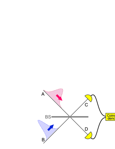
Figure 1: (color online) Two-photon interference at a $50/50$ beam splitter. Two independently prepared photons enters the two input ports $A$ and $B$ of the BS. They are eventually detected by two distinct detectors placed behind the output ports $C$ and $D$ of the BS. The plane of the figure is the plane of incidence

In the present work, the two independent photons impinging upon the $50/50$ BS are prepared in the product state $|\Psi^{AB}\rangle=|\Psi^{A}\rangle|\Psi^{B}\rangle$, where $|\Psi^{A}\rangle=\hat{a}^{\dagger}[\psi^{A}]|0\rangle$ ($|\Psi^{B}\rangle=\hat{b}^{\dagger}[\psi^{B}]|0\rangle$) denotes the single-photon state in arm $A$ ($B$), with $\hat{a}^{\dagger}[\psi^{A}]$ ($\hat{b}^{\dagger}[\psi^{B}]$) being the operator that creates one photon in the wavepacket mode (or, simply, wave function) $\psi^{A}$ ($\psi^{B}$) [17, 18]. The normalized wave functions $\psi^{A}$ and $\psi^{B}$ completely fix the spectral, polarization and spatiotemporal characteristics of the photon entering port $A$ and $B$, respectively.

Annihilation and creation operators associated to orthogonal wave functions, do commute: $\big{[}\hat{a}[\psi],\hat{b}^{\dagger}[\phi]\big{]}=\left(\psi,\phi\right)\delta_{ab}$, where $\left(\psi,\phi\right)$ denotes the scalar product in the complex linear space of the wave functions $\mathscr{L}\ni\psi,\phi$ [20]. The probability of detecting the two photons at the two output ports $C$ and $D$ is given by [21]:

$$P_{1,1}[\psi^{A},\psi^{B}]=\left(1-\left|\langle\Psi^{A}|\Psi^{B}\rangle\right|^{2}\right)/2,$$ (1)

where $\langle\Psi^{A}|\Psi^{B}\rangle=\left(\psi^{A},\psi^{B}\right)$.

Now, assume that the two input photons are prepared “almost” in the same manner, in such a way that they can be represented by the wave functions $\psi^{A}=\psi$ and $\psi^{B}=\left(\psi+\delta\psi\right)/\|\psi+\delta\psi\|\equiv\widetilde{\psi}+\widetilde{\delta\psi}$. The functional variation of the coincidence probability generated by $\delta\psi$ will be, by definition: $\Delta P_{1,1}[\psi]\equiv P_{1,1}[\psi,\widetilde{\psi}+\widetilde{\delta\psi}]-P_{1,1}[\psi,\psi]=P_{1,1}[\psi,\widetilde{\psi}+\widetilde{\delta\psi}]$, where $P_{1,1}[\psi,\psi]=0$ for identically prepared photons, as it trivially follows from (1) and normalization $\langle\Psi|\Psi\rangle=(\psi,\psi)=1$. A straightforward calculation from (1) yields

$$\Delta P_{1,1}[\psi]=\frac{1}{2}\frac{\Delta^{2}\left(1-|\alpha|^{2}\right)}{1+\Delta(\alpha+\alpha^{*})+\Delta^{2}},$$ (2)

where $\Delta^{2}\equiv(\delta\psi,\delta\psi)$, $\alpha\equiv(\psi,\delta\psi)/\Delta$ with $|\alpha|<1$ and $(\psi,\psi)=1$. This result is exact and rests on the basic properties of the scalar product in a complex linear space $\mathscr{L}$ solely.

Equation (2) may be further developed by assuming that the functional deviation $\delta\psi$ is generated by the variation of a single DOF, represented by the real parameter $f$, in such a way that $\psi^{A}=\psi(f)$ and $\psi^{B}=\psi(f+\delta\!f)$, with $|\delta\!f|\ll|f|$ and $\bigl{(}\psi(f),\psi(f)\bigr{)}=1$ for all $f$. For example, if $f=\nu$, the photon at input port $A$ has central frequency $\nu^{A}=\nu$ and the one entering port $B$ has central frequency $\nu^{B}=\nu+\delta\nu$. Defining $\delta\psi\equiv\psi(f+\delta\!f)-\psi(f)$ permits to express $\psi^{B}$ as above: $\psi^{B}=\psi+\delta\psi\equiv\widetilde{\psi}+\widetilde{\delta\psi}$. Formally expanding $\psi(f+\delta\!f)$ in powers of $\delta\!f$ as

$$\psi(f+\delta\!f)=\exp\left(\delta f\frac{\partial}{\partial f}\right)\psi(f)\simeq\psi(f)+\psi^{\prime}(f)\,{\delta f}+\psi^{\prime\prime}(f)\,\frac{{\delta f}\/^{\,2}}{2}+\dots,$$ (3)

with $\psi^{\prime}(f)=\partial\psi(f)/\partial f$, $\psi^{\prime\prime}(f)=\partial^{2}\psi(f)/\partial f^{2}$, et cetera, we can straightforwardly obtain

$$\Delta^{2}={\delta\!f}^{2}\Bigl{[}\left(\psi^{\prime},\psi^{\prime}\right)+\mathrm{Re}\left[\left(\psi^{\prime\prime},\psi^{\prime}\right)\right]\delta\!f+\Or({\delta\!f}^{2})\Bigr{]},$$ (4)

and $\alpha=\left[\left(\psi,\psi^{\prime}\right)+\left(\psi,\psi^{\prime\prime}\right)\delta\!f/2+\Or({\delta\!f}^{2})\right]/\Delta$. Since from (2) and (4) it follows that $\Delta P_{1,1}[\psi]\propto\Delta^{2}=\Or({\delta\!f}^{2})$, we define the rate of distinguishability $R_{f}[\psi]$ of the photons with respect to the degree of freedom $f$ via the relation

$$R_{f}[\psi] \equiv{\left.\frac{\partial^{2}}{\partial\,\delta\!f^{2}}P_{1,1}[\psi(f),\psi(f+\delta\!f)]\right|_{\delta\!f=0}}$$ (5)

$$=\left(\psi^{\prime},\psi^{\prime}\right)-|\left(\psi,\psi^{\prime}\right)|^{2},$$

where $0\leq R_{f}[\psi]\leq\|\psi^{\prime}\|^{2}$, and $\left(\psi,\psi^{\prime}\right)^{2}\leq 0$ because $0=\partial\left(\psi,\psi\right)/\partial f=\left(\psi,\psi^{\prime}\right)+\left(\psi^{\prime},\psi\right)$.

When defining the generator of a translation in the parameter $f$ as $\hat{K}=-\rmi\partial/\partial f$, one may understand the Taylor expansion (3) in terms of a propagator: $\psi(f+\delta\!f)=\exp(\rmi\delta\!f\hat{K})\psi(f)$. In general, $(\hat{K}\psi,\phi)\neq(\psi,\hat{K}\phi)$ for arbitrary wave functions $\psi$ and $\phi$ because $f$ is just a parameter upon which the photon wave function depends and not a dynamical variable. For this reason, the operator $\hat{K}$ is, in general, not self-adjoint. However, for some DOFs and certain states, e.g., spatial displacement of Gaussian states in wave vector representation, the relation $\left(\psi^{\prime},\psi^{\prime}\right)=-\left(\psi,\psi^{\prime\prime}\right)$ holds. In these cases the rate of indistinguishability $R_{f}[\psi]$ simplifies to the variance of $\hat{K}$, and we obtain a link to the geometry of quantum states [22].

The dimensionless parameter $R_{f}[\psi]\delta\!f^{2}$ has a straightforward physical meaning: it tells us how rapidly two identically prepared photons become distinguishable when we slightly vary, from $\psi(f)$ to $\psi(f+\delta\!f)$, the wave function of one photon with respect to the other. Thus, given a pair of photons prepared in the same state $|\Psi\rangle$, one can assert that they are maximally indistinguishable with respect to $f$ if $R_{f}[\psi]\leq R_{\bar{f}}[\psi]$ for any possible degree of freedom $\bar{f}$. In a complementary manner, provided two distinct pairs of photons, the first two photons being prepared in the state $|\Psi\rangle$ and the second ones in the state $|\Phi\rangle$, one can say that the photons in the first pair are maximally indistinguishable with respect to $\psi$ for a fixed $f$, if $R_{f}[\psi]\leq R_{f}[\phi]$ for all possible wave functions $\phi$. In this case it is not difficult to prove that the rate of distinguishability is minimal for a Gaussian shaped wave function [23]. In summary: “all photons are equal but some photons are more equal than others” , and $R_{f}[\psi]$ quantifies the degree of equality.

This result concludes the first part of this work. Next, we will apply equations (3) and (4) to the realistic case of optical Gaussian wave packets with well-defined spectral, spatiotemporal and polarization DOFs.

3 Gaussian wave packets.

Consider a single-photon wave packet of the form:

$$\left|\Psi\right>=\sum_{s=1}^{2}{\int}\rmd^{3}k\,\psi_{s}(\bi{k})\hat{a}^{\dagger}_{s}(\bi{k})\left|0\right>,$$ (6)

where $\left|0\right>$ denotes the ground state of the continuous Fock space and $\hat{a}_{s}(\bi{k})$ is the operator that annihilates one photon from the plane wave mode $\bi{e}_{s}(\bi{k})\exp\left(\rmi\bi{k}\cdot\bi{r}\right)$, with $\bigl{[}\hat{a}_{s}(\bi{k}),\hat{a}^{\dagger}_{s^{\prime}}(\bi{k}^{\prime})\bigr{]}=\delta^{(3)}(\bi{k}-\bi{k}^{\prime})\delta_{ss^{\prime}}$ [24]. Here $\left\{\bi{e}_{1}(\bi{k}),\bi{e}_{2}(\bi{k}),\bi{k}/\left|\bi{k}\right|\right\}$ denotes a right-handed orthonormal basis set attached to the wave vector $\bi{k}$. The normalization of the state is ensured by requiring $\langle\Psi|\Psi\rangle=\sum_{s=1}^{2}{\int}\rmd^{3}k\,|\psi_{s}(\bi{k})|^{2}=1$. The spectral amplitudes $\psi_{s}(\bi{k})$ ($s=1,2$) determine the shape and the polarization of the beam. They may be obtained by imposing the quantum-classical correspondence

$$\langle 0|\hat{\bi{E}}^{(+)}(\bi{r},t)|\Psi\rangle=\bi{E}^{(+)}_{\rm{cl}}(\bi{r},t),$$ (7)

where $\bi{E}^{(+)}_{\rm{cl}}(\bi{r},t)$ is the positive-frequency part of the classical field wave packet whose energy equals the mean energy of the photon in the state $|\Psi\rangle$, and

$$\eqalign{\hat{\bi{E}}^{(+)}(\bi{r},t)=&\frac{\rmi}{(2\pi)^{3/2}}\sum_{s=1}^{2}\int\rmd^{3}k\,\sqrt{\frac{\hbar\omega}{2\epsilon_{0}}}\hat{a}_{s}(\bi{k})\bi{e}_{s}(\bi{k})\exp\left[\rmi\left(\bi{k}\cdot\bi{r}-\omega t\right)\right],}$$ (8)

with $\omega=c\left|\bi{k}\right|\equiv ck$, $c$ being the speed of light in vacuum and $\epsilon_{0}$ the vacuum permittivity. The expression for $\bi{E}^{(+)}_{\rm{cl}}(\bi{r},t)$ is given by the right side of (8) with the quantum operator $\hat{a}_{s}(\bi{k})$ replaced by the classical amplitude $\tilde{a}_{s}(\bi{k})$. Then, by substituting from equations (6) and (8) into (7), one attains $\psi_{s}(\bi{k})=\tilde{a}_{s}(\bi{k})$. The total energy contained in such wave packet is given by $\mathcal{E}=\int\rmd^{3}k\,\hbar\omega\left(\left|\tilde{a}_{1}(\bi{k})\right|^{2}+\left|\tilde{a}_{2}(\bi{k})\right|^{2}\right)$.

Without loss of generality, we assume that $\tilde{a}_{s}(\bi{k})=\varepsilon_{s}(\bi{k})E(\bi{k})$, where $E(\bi{k})$ and $\varepsilon_{s}(\bi{k})$ are the scalar and the vector spectral amplitudes of the field, respectively. $E(\bi{k})$ determines the spatial characteristics of the field, and $\varepsilon_{s}(\bi{k})$ the polarization ones. Here we consider a collimated, quasi-monochromatic wave packet, with central wave vector $\bi{k}_{0}$ and central frequency $\omega_{0}=c\left|\bi{k}_{0}\right|\equiv ck_{0}$. We choose a normalized Gaussian spectral amplitude $E(\bi{k})=\gamma(\bi{k}-\bi{k}_{0})$, where

$$\gamma(\bi{q})=\frac{(\det V)^{1/4}}{\pi^{3/4}}\exp\left[-\rmi\;\bi{q}\cdot\bi{r}_{0}-\frac{1}{2}\;\bi{q}\cdot V\bi{q}\right],$$ (9)

with $V^{-1}=\mathrm{diag}\left(\sigma_{1}^{2},\sigma_{2}^{2},\sigma_{3}^{2}\right)$. This choice for $V$ yields a factorizable spectral amplitude $\gamma(\bi{q})=g(q_{1})g(q_{2})g(q_{3})$ with $g(q_{n})=\exp[-\rmi q_{n}r_{0n}-q_{n}^{2}/(2\sigma_{n}^{2})]/(\pi^{1/4}\sqrt{\sigma_{n}})$. Clearly, it is possible to consider a more general positive definite symmetric matrix $V$ that couples different wave vector coordinates. We will see later that such a coupling may have dramatic consequences upon the rate of distinguishability of photons. In (9) the real vector $\bi{r}_{0}=\{r_{01},r_{02},r_{03}\}$ gives the position, at time $t=0$, of the center of the wave packet. We fix $\varepsilon_{s}(\bi{k})$ assuming that the wave packet has passed across a polarizer that selects a uniform field polarization parallel to $\bi{p}\in\mathbb{C}^{3}$ and perpendicular to $\bi{k}_{0}$, with $\left|\bi{p}\right|^{2}=1$ and $\bi{k}_{0}\cdot\bi{p}=0$. In this case, it becomes natural to define $\varepsilon_{s}(\bi{k})$ as the normalized projection of $\bi{p}$ upon $\bi{e}_{s}(\bi{k})$, namely [25, 26]: $\varepsilon_{s}(\bi{k})={\bi{e}_{s}(\bi{k})\cdot\bi{p}}/{\sqrt{1-|(\bi{p},\bi{k})|^{2}/k^{2}}}$, with $\left|\varepsilon_{1}(\bi{k})\right|^{2}+\left|\varepsilon_{2}(\bi{k})\right|^{2}=1$ by definition.

The Gaussian distribution $\gamma(\bi{k}-\bi{k}_{0})$ implies that the wave packet is concentrated in a region of the $\bi{k}$-space of “volume” $\sigma_{1}\sigma_{2}\sigma_{3}$ centered at $\bi{k}_{0}$. Then, the assumptions of collimation and quasi-monochromaticity entail the constraints $\sigma_{i}\ll k_{0},\;(i=1,2,3)$. In this case, the total energy of the wave packet can be written as $\mathcal{E}=\int\rmd^{3}k\,\hbar\omega\left|\gamma(\bi{k}-\bi{k}_{0})\right|^{2}\simeq\hbar\omega_{0}$, where $\int\rmd^{3}k\,\left|\gamma(\bi{k}-\bi{k}_{0})\right|^{2}=1$ by definition.

For quasi-monochromatic and collimated beams the Gaussian spectral amplitude $\psi_{s}(\bi{k})=\varepsilon_{s}(\bi{k})\gamma(\bi{k}-\bi{k}_{0})$ contains $(3+3)+3+3=12$ independent real parameters corresponding to the (spectral) $\oplus$ spatial $\oplus$ polarization DOFs: $\left(\bi{k}_{0}\,\oplus\{\sigma_{1},\sigma_{2},\sigma_{3}\}\right)\,\oplus\bi{r}_{0}\,\oplus\{\bi{p}\in\mathbb{C}^{3}:\left|\bi{p}\right|^{2}=1\,\wedge\,\bi{k}_{0}\cdot\bi{p}=0\}$. Note that the central frequency $\omega_{0}$ is not an additional independent parameter, since $\omega_{0}=c\left|\bi{k}_{0}\right|$. Each of these $12$ (actually $15$ if we consider a non-diagonal symmetric $V$) parameters can be taken as the variable $f$ to evaluate the rate of distinguishability $R_{f}[\psi]$. This calculation will be the goal of the remainder.

4 Rate of distinguishability

Using rather standard methods of calculation [27, 28], it is not difficult to show that the coincidence probability (1) can be expressed in terms of the spectral amplitudes $\psi_{s}^{A}(\bi{k})$ and $\psi_{s}^{B}(\bi{k})$ of the input photons as

$$\!\!\!P_{1,1}[\psi^{A},\psi^{B}]=\frac{1}{2}\!\left[1-\biggl{|}\sum_{s=1}^{2}{\int}\rmd^{3}k\,{\psi_{s}^{A}(\bi{k})\psi_{s}^{B}}^{*}(\underline{\bi{k}})\biggr{|}^{2}\right],$$ (10)

where $\underline{\bi{k}}$ has components $\{-k_{1},k_{2},k_{3}\}$. This change of sign in the $1$-coordinate is due to the parity inversion occurring by reflection at the BS. Hereafter, we assume two Gaussian wave packets $\psi_{s}^{A}(\bi{k})=\psi_{s}(\bi{k},f)$ and $\psi_{s}^{B}(\bi{k})=\psi_{s}(\bi{\underline{k}\,},f+\delta\!f)$. Moreover, for concreteness, we choose the $3$-axis of the Cartesian reference frame directed along $\bi{k}_{0}$, namely $\bi{k}_{0}=\{0,0,k_{0}\}$.

The explicit values of $R_{f}$, calculated from (5), are given in table 1 below, for spectral and spatial DOFs:

Table 1: Rate of distinguishability $\displaystyle{R_{f}}$ for several spectral and spatial degrees of freedom $f$ of the photons, with $n=1,2,3$.

• $f$	$k_{0n}$	$\sigma_{n}$	$r_{0n}$
  $\displaystyle{R_{f}}$	$\displaystyle{\frac{1}{2\sigma_{n}^{2}}}$	$\displaystyle{\frac{1}{2\sigma_{n}^{2}}}$	$\displaystyle{\frac{\sigma_{n}^{2}}{2}}$

A remarkable consequence from table 1, is that for the complementary position$/$wave-vector variables, the following Fourier-transform equality holds:

$$R_{k_{0n}}R_{r_{0n}}={1}/{4},\qquad\forall\,n=1,2,3.$$ (11)

table 1 furnishes some valuable information. Consider, for example, the last column: it shows that $R_{r_{0n}}^{1/2}{\delta r_{0n}}$ is equal to the ratio between the variation $\delta r_{0n}$ and the standard deviation (square root of the variance) $\sqrt{2}/\sigma_{n}$ of the absolute value squared of the photon wave function in configuration space. This is in agreement with intuition: imagine the cross-section of each photon as a disc of radius $\sqrt{2}/\sigma_{n}$. Starting from an initial condition of perfect superposition between the two discs, suppose to shift one disc with respect to the other by the amount ${\delta r_{0n}}$. Now, if ${\delta r_{0n}}\ll\sqrt{2}/\sigma_{n}$ the two discs have still a large superposition and the two photons remain largely indistinguishable. Vice versa, if ${\delta r_{0n}}\sim\sqrt{2}/\sigma_{n}$ the two discs separate completely and the superposition drops to zero. In this case the photons become “quickly” distinguishable. Analogous reasonings may be reproduced for the other DOFs.

Next, we consider the case of a non-factorable spectral amplitude, which couples wave vector coordinates $1$ and $2$. Equation (9) still holds, but now $V$ has diagonal and non diagonal elements $V_{nm}=\delta_{nm}/\sigma^{2}_{n}-(\delta_{n1}\delta_{m2}+\delta_{n2}\delta_{m1})/\sigma_{nm}$, where the real parameter $\sigma_{12}$ establishes the coupling, with $\sigma_{12}^{2}>\sigma_{1}^{2}\sigma_{2}^{2}$ as required by positive definiteness of $V$. A straightforward calculation furnishes

$$R_{\sigma_{n}}=\frac{1}{2\sigma_{n}^{2}}\frac{1}{(1-\rho^{2})^{2}},\qquad(n=1,2),$$ (12)

where $\rho\equiv\sigma_{1}\sigma_{2}/\sigma_{12}$, with $\left|\rho\right|<1$. If $\rho=0$ (uncoupled DOFs) we recover the results of table 1. Vice versa, for increasing coupling one has $\rho\;\rightarrow\;1$ and $R_{\sigma_{n}}$ grows unboundedly. This result is of particular relevance to experimentalists: it tells us that wave packets whose cross section has the shape of an ellipse whose either major or minor axis does not lay on the plane of incidence (see figure 1), are much more sensitive to mode-mismatch than cylindrically symmetric wave packets. This occurrence strongly degrades photon indistinguishability and should be avoided, for example, in coalescence experiments [12, 13].

Finally, we examine the polarization DOFs of the two photons. Let us parameterize $\bi{p}^{A}$ and $\bi{p}^{B}$ as $\bi{p}^{\lambda}=\left\{\cos\vartheta^{\lambda}\exp\left(i\varphi^{\lambda}_{1}\right),\,\sin\vartheta^{\lambda}\exp\left(i\varphi^{\lambda}_{2}\right),0\right\}$, with $\lambda=A,B$ and $|\bi{p}^{A}|=|\bi{p}^{B}|=1$. The results, as expansions in powers of $\sigma_{1},\sigma_{2}$, are

$$R_{\vartheta} \simeq 1+\frac{\sigma_{1}^{2}-\sigma_{2}^{2}}{2k_{0}^{2}}\cos(2\vartheta)+\dots,$$ (13a)

$$R_{\varphi_{n}} \simeq\frac{\sin^{2}(2\vartheta)}{4}\left[1+\frac{\sigma_{1}^{2}-\sigma_{2}^{2}}{2k_{0}^{2}}\cos(2\vartheta)+\dots\right],$$ (13b)

with $n=1,2$. Unlike in the spectral and the scalar cases, $R_{\vartheta}$ and $R_{\varphi_{n}}$ are dimensionless quantities. From a physical point of view, this means that there is not a natural scale for the variation of the polarization DOFs. From equations (13) one sees that for astigmatic wave packets, namely for $\sigma_{1}\neq\sigma_{2}$, there is a coupling between spectral and polarization DOFs that affects in equal manner both $R_{\vartheta}$ and $R_{\varphi_{n}}$. The term $(\sigma_{1}^{2}-\sigma_{2}^{2})/{(2k_{0}^{2})}$ may be interpreted as a manifestation of the unavoidable spin-orbit coupling occurring in transverse electromagnetic fields [31]. In addition, its absolute value furnishes the visibility of the coincidence fringes [32]. Equation (13b) shows that $R_{\varphi_{n}}\propto\sin^{2}(2\vartheta)$. As a consequence, for linearly polarized states with $2\vartheta=0,\pm\pi,\pm 2\pi,\dots$, the phase is not a relevant DOF and $R_{\varphi_{n}}=0$.

By definition, the rate of distinguishability $R_{f}[\psi]$ can be measured by interfering two independently created photons, each prepared in a state tunable in one specific DOF $f$. Such experiments have been realized for longitudinal spatiotemporal displacement $f=r_{03}$ [29] and central frequency $f=k_{03}$ [30]. Plotting the coincidence probability $P_{1,1}$ against the variation $\delta\!f$, yields a curve with a dip centered around $\delta\!f=0$. By fitting this dip with a parabolic curve, as depicted in figure (2), one can straightforwardly extract $R_{f}[\psi]$ from the experimental data.

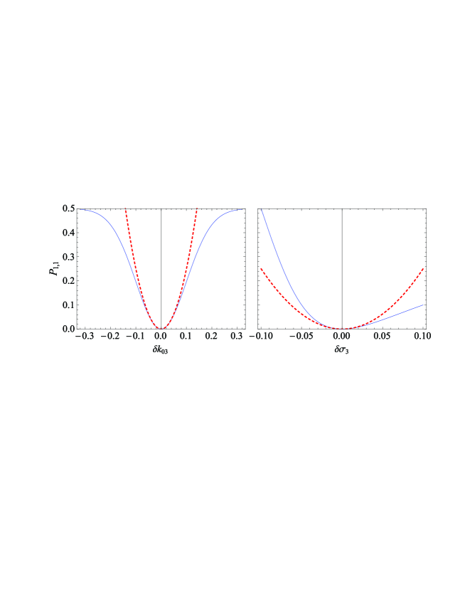
Figure 2: (color online) Coincidence probability $P_{1,1}$ for $f=k_{03}$ (left) and $f=\sigma_{3}$ (right). Blue lines: from equations (9) and (10); dashed red lines: $R_{f}\delta\!f^{2}/2$. In both plots we fixed $\sigma_{3}/k_{03}=1/10$.

5 Mixed States

In this section we consider the case occurring when both photons at the input ports of the BS are prepared in a statistical mixture. This is of great practical relevance especially for quantum information processing applications. We shall see that in certain circumstances there are profound differences for the rate of distinguishability of photons, as compared to the pure states case.

For statistical mixtures equation (1), describing the probability of detecting the two photons at the two output ports $C$ and $D$, generalizes to:

$$P_{1,1}\left[\hat{\rho}^{A},\hat{\rho}^{B}\right]=\frac{1}{2}\left(1-\mathrm{Tr}\big{[}\hat{\rho}^{A}\hat{\rho}^{B}\big{]}\right),$$ (13n)

where $\mathrm{Tr}[\dots]$ denotes the trace operation and $\hat{\rho}^{A},\hat{\rho}^{B}$ are the normalized density operators describing the quantum state of photon $A$ and $B$ respectively. Differently from the pure state case where one has $P_{1,1}\left[\psi,\psi\right]=0$, now

$$P_{1,1}\left[\hat{\rho},\hat{\rho}\right]=\frac{1}{2}\left(1-\mathrm{Tr}\big{[}\hat{\rho}^{2}\big{]}\right),$$ (13o)

which is nonzero except for a pure state where $\mathrm{Tr}\big{[}\hat{\rho}^{2}\big{]}=\mathrm{Tr}\big{[}\hat{\rho}\big{]}=1$. Now we proceed by analogy with the pure state case by choosing $\hat{\rho}^{A}=\hat{\rho}$ and

$$\hat{\rho}^{B}=\frac{\hat{\rho}+\delta\hat{\rho}}{1+\mathrm{Tr}\left[\delta\hat{\rho}\right]},$$ (13p)

where with $\delta\hat{\rho}$ we denoted the (supposedly small) variation of $\hat{\rho}$. By using (13o) and (13p) one can calculate the difference $\Delta P_{1,1}\left[\hat{\rho}\right]\equiv P_{1,1}\left[\hat{\rho},\frac{\hat{\rho}+\delta\hat{\rho}}{1+\mathrm{Tr}\left[\delta\hat{\rho}\right]}\right]-P_{1,1}\left[\hat{\rho},\hat{\rho}\right]$ as a perturbation expansion with respect to $\mathrm{Tr}[\delta\hat{\rho}]$ by noting that for $\mathrm{Tr}[\delta\hat{\rho}]<1$ equation (13p) may be written as a geometrical series:

$$\Delta P_{1,1}\left[\hat{\rho}\right]=\frac{1}{2}\left(\mathrm{Tr}[\hat{\rho}^{2}]\,\mathrm{Tr}[\delta\hat{\rho}]-\mathrm{Tr}[\hat{\rho}\,\delta\hat{\rho}]\right)\left(1-\mathrm{Tr}[\delta\hat{\rho}]+\mathrm{Tr}[\delta\hat{\rho}]^{2}-\dots\right).$$ (13q)

Here an apparently striking difference with respect to the pure states case occurs: the first variation of $P_{1,1}$ is linear in $\delta\hat{\rho}$. Moreover, if one chooses $\delta\hat{\rho}$ such that $\mathrm{Tr}[\delta\hat{\rho}]=0$ (we shall see later when this naturally occurs), then (13q) reduces exactly to:

$$\Delta P_{1,1}\left[\hat{\rho}\right]=-\frac{1}{2}\mathrm{Tr}[\hat{\rho}\,\delta\hat{\rho}]=-\frac{1}{2}\left\langle\delta\hat{\rho}\right\rangle.$$ (13r)

Moreover, it is not difficult to see that when the photons are prepared in pure states, so that one chooses $\hat{\rho}^{A}=|\Psi\rangle\langle\Psi|$, with $\langle\Psi|\Psi\rangle=1$, and

$$\hat{\rho}^{B}=\frac{\left(|\Psi\rangle+|\delta\Psi\rangle\right)\left(\langle\Psi|+\langle\delta\Psi|\right)}{1+\langle\Psi|\delta\Psi\rangle+\langle\delta\Psi|\Psi\rangle+\langle\delta\Psi|\delta\Psi\rangle},$$ (13s)

then the first “linear” term on the right side of equation (13q) becomes

$$\frac{1}{2}\left(\mathrm{Tr}[\hat{\rho}^{2}]\,\mathrm{Tr}[\delta\hat{\rho}]-\mathrm{Tr}[\hat{\rho}\,\delta\hat{\rho}]\right) =\frac{1}{2}\Big{[}\langle\delta\Psi|\delta\Psi\rangle-\left|\langle\Psi|\delta\Psi\rangle\right|^{2}\Big{]}$$ (13t)

$$=\frac{1}{2}\Big{[}(\delta\psi,\delta\psi)-\left|(\psi,\delta\psi)\right|^{2}\Big{]},$$

which is clearly quadratic in $\delta\psi$ and we recover the results of section 2.

The second relevant difference between statistical mixtures and pure states is that in the first case we have at our disposal also the parameters of the statistical distribution of the pure states (which constitute the ensemble characterizing the photons) to yield the variation $\delta\hat{\rho}$, in addition to the “deterministic” DOFs $f$ used previously. Specifically, we can distinguish amongst two different cases: given

$$\hat{\rho}^{A}=\sum_{n}w_{n}|\Phi_{n}(f)\rangle\langle\Phi_{n}(f)|,$$ (13u)

with $w_{n}\geq 0$, $\sum_{n}w_{n}=1$ and $\langle\Phi_{n}(f)|\Phi_{m}(f)\rangle=\delta_{nm}$, we can choose $\hat{\rho}^{B}$ either a) by varying the statistical distribution $w_{n}\rightarrow w_{n}+\delta w_{n}$, or b) by varying the DOFs $f$ of the wave packet, namely $\left|\Phi_{n}(f)\right>\rightarrow\left|\Phi_{n}(f+\delta\!f)\right>$.

Case a): Let

$$\hat{\rho}^{A}=\sum_{n}w_{n}|\Phi_{n}\rangle\langle\Phi_{n}|\equiv\hat{\rho}\mathrm{~{}~{}and~{}~{}}\hat{\rho}^{B}=\sum_{n}\frac{w_{n}+\delta w_{n}}{1+\sum_{m}\delta w_{m}}|\Phi_{n}\rangle\langle\Phi_{n}|,$$ (13v)

represent the quantum states of photons $A$ and $B$, respectively. Then, a straightforward calculation yields, up to and including second order terms,

$$\Delta P_{1,1}\left[\hat{\rho}\right]=\frac{1}{2}\sum_{n}\delta w_{n}\left(\mathrm{Tr}[\hat{\rho}^{2}]-w_{n}\right)\Bigl{[}1-\sum_{m}\delta w_{m}+\dots\Bigr{]}.$$ (13w)

Here, the first (linear) term is, in general, non zero. A notable case occurs for $N$-dimensional maximally mixed states where $w_{n}=1/N$ for all $n$ and $\mathrm{Tr}[\hat{\rho}^{2}]=1/N\Rightarrow\Delta P_{1,1}\left[\hat{\rho}\right]=0$. Physically, this means that photons prepared in maximally mixed states are intrinsically more robust against “distinguishability” than photons in pure states. However, the indistinguishability of maximally mixed states is per se very poor since for them $P_{1,1}[\hat{\rho},\hat{\rho}]=(1-1/N)/2$.

Case b): In this case we have

$$\hat{\rho}^{A}= \;\sum_{n}w_{n}|\Phi_{n}(f)\rangle\langle\Phi_{n}(f)|\equiv\hat{\rho}(f),$$ (13xa)

$$\hat{\rho}^{B}= \;\sum_{n}w_{n}|\Phi_{n}(f+\delta\!f)\rangle\langle\Phi_{n}(f+\delta\!f)|\equiv\hat{\rho}(f+\delta\!f),$$ (13xb)

with $\delta\hat{\rho}=\hat{\rho}^{B}-\hat{\rho}^{A}$ such that $\mathrm{Tr}[\delta\hat{\rho}]=0$ as follows from normalization condition: $\langle\Phi_{n}(f)|\Phi_{n}(f)\rangle=1$ for all $f$ or, equivalently, $\mathrm{Tr}[\hat{\rho}(f)]=1=\mathrm{Tr}[\hat{\rho}(f+\delta\!f)]$. The variation $\delta\hat{\rho}=\hat{\rho}(f+\delta\!f)-\hat{\rho}(f)$ can be written as a Taylor expansion

$$\delta\hat{\rho}=\delta\!f\frac{\partial\hat{\rho}}{\partial f}+\frac{\delta\!f^{2}}{2}\frac{\partial^{2}\hat{\rho}}{\partial f^{2}}+\dots,$$ (13xy)

and substituted into (13r) to calculate

$$\Delta P_{1,1}\left[\hat{\rho}\right]=-\frac{1}{2}\left\langle\delta\hat{\rho}\right\rangle=-\frac{1}{2}\left[\delta\!f\left\langle\frac{\partial\hat{\rho}}{\partial f}\right\rangle+\frac{\delta\!f^{2}}{2}\left\langle\frac{\partial^{2}\hat{\rho}}{\partial f^{2}}\right\rangle+\dots\right],$$ (13xz)

where $\langle\hat{O}\rangle$ denotes $\mathrm{Tr}[\hat{\rho}\,\hat{O}]$. By using the evident relation

$$\frac{\partial}{\partial f}\langle\Phi_{n}(f)|\Phi_{n}(f)\rangle=0,$$ (13xaa)

it is not difficult to prove that

$$\left\langle\frac{\partial\hat{\rho}}{\partial f}\right\rangle=0.$$ (13xab)

Thus, (13xz) can be rewritten as

$$\Delta P_{1,1}\left[\hat{\rho}\right]=-\frac{\delta\!f^{2}}{4}\left\langle\frac{\partial^{2}\hat{\rho}}{\partial f^{2}}\right\rangle+\dots.$$ (13xac)

Equation (13xac) shows that for case b), namely when we vary one DOF of the photon state, say $f$, the variation $\Delta P_{1,1}$ of the probability coincidence is at least of the second order with respect to $\delta\!f$. This result not only reproduces our findings in section 2, but extend their validity to the case of mixed states. Of course, (13xac) is also valid for pure states and, therefore, we can rewrite the rate of distinguishability as proportional to the expectation value of the operator $\partial^{2}\hat{\rho}/\partial f^{2}$:

$$R_{f}\left[\hat{\rho}\right]=-\frac{1}{2}\left\langle\frac{\partial^{2}\hat{\rho}}{\partial f^{2}}\right\rangle.$$ (13xad)

Let us apply the results obtained above to the exactly tractable case of a partially polarized paraxial beam of light prepared in a well defined spatial mode decoupled from polarization DOFs. The relevant single-photon density operator is given by

$$\hat{\rho}=\hat{\rho}(\alpha,\vartheta,\varphi)=\cos^{2}\alpha|\Psi\rangle\langle\Psi|+\sin^{2}\alpha|\Psi_{\perp}\rangle\langle\Psi_{\perp}|,$$ (13xae)

where $\alpha\in[0,2\pi[$ and

$$|\Psi\rangle=\cos\vartheta|x\rangle+\sin\vartheta\,e^{i\varphi}|y\rangle\mathrm{~{}~{}and~{}~{}}|\Psi_{\perp}\rangle=-\sin\vartheta\,e^{-i\varphi}|x\rangle+\cos\vartheta|y\rangle,$$ (13xaf)

with $|x\rangle$ and $|y\rangle$ representing two normalized orthogonal polarization states: $\langle x|y\rangle=0$. According to the preceding analysis, we can study two different cases:

$$\mathrm{{\it a})}\quad\left\{\begin{array}[]{ll}\hat{\rho}^{A}&=\hat{\rho}(\alpha,\vartheta,\varphi),\\ \hat{\rho}^{B}&=\hat{\rho}(\alpha+\delta\alpha,\vartheta,\varphi),\\ \end{array}\right.\qquad\mathrm{{\it b})}\quad\left\{\begin{array}[]{ll}\hat{\rho}^{A}&=\hat{\rho}(\alpha,\vartheta,\varphi),\\ \hat{\rho}^{B}&=\hat{\rho}(\alpha,\vartheta+\delta\vartheta,\varphi).\\ \end{array}\right.$$ (13xak)

For case a) a straightforward calculation furnishes

$$\Delta P_{1,1}\left[\hat{\rho}\right] =\frac{1}{4}\sin(\delta\alpha)\left[\sin(\delta\alpha)+\sin(4\alpha+\delta\alpha)\right]$$ (13xal)

$$=\frac{\delta\alpha}{4}\sin(4\alpha)+\frac{\delta\alpha^{2}}{2}\cos^{2}(2\alpha)+\dots.$$

Equation (13xal) shows that as a consequence of the variation of the parameter $\alpha$ defining the statistical distribution of the mixed state, the corresponding variation of $\Delta P_{1,1}$ is linear in $\delta\alpha$ and the “quadratic” rate of distinguishability cannot be defined here. However, it should be noticed that our rate of distinguishability coincides with the second order coefficient of the Taylor expansion of $\Delta P_{1,1}$. Therefore, in principle, if one identifies the $n$th order coefficient of such expansion with the $n$th rate of distinguishability $R_{f}^{(n)}$ (with $R_{f}=R_{f}^{(2)}$) a hierarchy between $n$th and $(n+1)$th rate of distinguishability is unambiguously established. Thus, for example, in the case above the existence of the first order rate of distinguishability $R_{f}^{(1)}=\sin(4\alpha)/4$ indicates a greater attitude of photons to become distinguishable when there statistical distribution is varied. Note that, as expected, for the maximally mixed state attained at $\alpha=\pi/4$ one has exactly $\Delta P_{1,1}\left[\hat{\rho}\right]=0$, as previously found on the ground of general considerations.

For case b) we put $f=\vartheta$ and obtain

$$\Delta P_{1,1}\left[\hat{\rho}\right] =\frac{1}{2}\cos^{2}(2\alpha)\sin^{2}(\delta\vartheta)$$ (13xam)

$$=\frac{\delta\vartheta^{2}}{2}\cos^{2}(2\alpha)+\dots.$$

By an explicit calculation one can see that (13xam) is in perfect agreement with (13xad). Moreover, once again, for $\alpha=\pi/4$ one retrieve the expected result $\Delta P_{1,1}\left[\hat{\rho}\right]=0$. For pure states occurring at $\alpha\in\{0,\pi/2,\pi,3\pi/2\}$ this result does also coincide with (13a) which furnishes $R_{\vartheta}=1$ in absence of spin-orbit coupling.

6 Conclusions

In this work we have investigated photon distinguishability from an operational point of view. We introduced a new parameter, the rate of distinguishability $R_{f}[\psi]$, which furnishes a quantitative measure of the distinguishability of photons (prepared in the state $|\Psi\rangle$) with respect to the DOF $f$. Our main results are summarized by Equations (2,5,12,13xad), and table 1. In particular, (12) quantifies the degradation of photon distinguishability due to coupling between different DOFs. Moreover, we extended the definition of $R_{f}[\psi]$ form the pure state $\left|\Psi\right>$ to the density operator $\hat{\rho}$. For this case we found that the variation of the statistical distribution of the incoming photons affects their degree of distinguishability which is, in practice, increased. As a final remark, we stress that $R_{f}[\psi]$ is experimentally accessible via the measurement of the two-photon coincidence probability.

References

References

• [1] Knill E Laflamme R and Milburn G J 2001 Nature 409 46
• [2] Ray M R and van Enk S J 2011 Phys. Rev. A 83 042318
• [3] Gavenda M, Čelechovská L, Soubusta J, Dušek M and R Filip 2011 Phys. Rev. A 83 042320
• [4] Nielsen M A and Chuang I L 2010 Quantum Computation and Quantum Information (Cambridge: University Press Cambridge)
• [5] Souza C E R, Borges C V S, Khoury A Z, Huguenin J A O, Aolita L and Walborn S P 2008 Phys. Rev. A 77 032345
• [6] Keller M, Lange B, Hayasaka K, Lange W and Walther H 2004 Nature 431 1075
• [7] McKeever J, Boca A, D Boozer A, Miller R, Buck J R, Kuzmich A and Kimble H J 2004 Science 303 1992
• [8] Kuhn A, Hennrich M and Rempe G 2002 Phys. Rev. Lett. 89 067901
• [9] Bochmann J, Mücke M, Langfahl-Klabes G, Erbel C, Weber B, Specht H P, Moehring D L and Rempe G 2008 Phys. Rev. Lett. 101 223601
• [10] Kolchin P, Belthangady C, Du S, Yin G Y and Harris S E 2008 Phys. Rev. Lett. 101 103601
• [11] Wilk T, Webster S C, Specht H P, Rempe G and Kuhn A 2007 Phys. Rev. Lett. 98 063601
• [12] Legero T, Wilk T, Hennrich M, Rempe G and Kuhn A 2004 Phys. Rev. Lett. 93 070503
• [13] Specht H P, Bochmann J, Mücke M, Weber B, Figueroa E, Moehring D L and Rempe G 2009 Nature Phot 3 469
• [14] Hong C K, Ou Z Y and Mandel L 1987 Phys. Rev. Lett. 59 2044
• [15] Kaltenbaek R, Lavoie J, and Resch K J 2009 Phys. Rev. Lett. 102 243601
• [16] Flagg E B, Muller A, Polyakov S V, Ling A, Migdall A and Solomon G S 2010 Phys. Rev. Lett. 104 137401
• [17] Deutsch I H 1991 Am. J. Phys. 59 834
• [18] Loudon R 1998 Phys. Rev. A 58 4904
• [19] Merzbacher E 1998 Quantum Mechanics 3rd Ed. (New York: John Wiley & Sons, Inc.)
• [20] Kolmogorov A N and Fomin S V 1975 Introductory Real Analysis (Mineola, NY: Dover Publications, Inc.)
• [21] Loudon R 2000 The Quantum Theory of Light (Oxford: University Press Oxford)
• [22] Anandan J and Aharonov Y 1990 Phys. Rev. Lett. 65 1697
• [23] Rohde P P, Ralph T C and Nielsen M A 2005 Phys. Rev. A 72 052332
• [24] Mandel L and Wolf E 1995 Optical Coherence and Quantum Optics (Cambridge: University Press Cambridge)
• [25] Fainman Y and Shamir J 1984 Appl. Opt. 23 3188
• [26] Aiello A, Marquardt Ch and Leuchs G 2009 Opt. Lett. 34 3160
• [27] Walborn S P, de Oliveira A N, Pádua S and Monken C H 2003 Phys. Rev. Lett. 90 143601
• [28] Deng L P, Dang G F and Wang K 2006 Phys. Rev. A 74 063819
• [29] Beugnon J, Jones M P A, Dingjan J, Darquié B, Messin G, Browaeys A and Grangier P 2006 Nature 440 779
• [30] Legero T, Wilk T, Kuhn A and Rempe G 2006 Advances in Atomic Molecular and Optical Physics 53 253
• [31] Bliokh K Y, Alonso M A, Ostrovskaya E A and Aiello A 2010 Phys. Rev. A 82 063825
• [32] Nogueira W A T, Santibañez M, Pádua S, Delgado A, Saavedra C, Neves L and Lima G 2010 Phys. Rev. A 82 042104