Multifractal analysis of complex networks
Abstract
Complex networks have recently attracted much attention in diverse areas of science and technology. Many networks such as the WWW and biological networks are known to display spatial heterogeneity which can be characterized by their fractal dimensions. Multifractal analysis is a useful way to systematically describe the spatial heterogeneity of both theoretical and experimental fractal patterns. In this paper, we introduce a new box covering algorithm for multifractal analysis of complex networks. This algorithm is used to calculate the generalized fractal dimensions of some theoretical networks, namely scale-free networks, small world networks and random networks, and one kind of real networks, namely protein-protein interaction networks of different species. Our numerical results indicate the existence of multifractality in scale-free networks and protein-protein interaction networks, while the multifractal behavior is not clear-cut for small world networks and random networks. The possible variation of due to changes in the parameters of the theoretical network models is also discussed.
Key words: Complex networks; multifractality; box covering algorithm.
1 Introduction
Complex networks have been studied extensively due to their relevance to many real-world systems such as the world-wide web, the internet, energy landscapes, and biological and social systems.
It has been shown that many real complex networks share distinct characteristics that differ in many ways from random and regular networks. Three fundamental properties of real complex networks have attracted much attention recently: the small-world property, the scale-free property,[6-8] and the self-similarity. The small-world property means that the average shortest path length between vertices in the network is short, usually scaling logarithmically with the size of the network. A famous example is the so-called six degrees of separation in social networks. A large number of real networks are referred to as scale-free because the probability distribution of the number of links per node (also known as the degree distribution) satisfies a power law with the degree exponent varying in the range . In view of their small-world property, it was believed that complex networks are not self-similar under a length-scale transformation. After analyzing a variety of real complex networks, Song et al. found that they consist of self-repeating patterns on all length scales, i.e., they have self-similar structures. In order to unfold the self-similar property of complex networks, Song et al. calculated their fractal dimension, a known useful characteristic of complex fractal sets,[9-11] and found that the box-counting method is a proper tool for further investigations of network properties. Because a concept of metric on graphs is not as straightforward as the Euclidean metric on Euclidean spaces, the computation of the fractal dimension of networks via a box-counting approach is much more complicated than the traditional box-counting algorithm for fractal sets in Euclidean spaces. Actually Eguiluz et al. introduced appropriate definitions of dimensions in order to characterize the fractal properties of complex networks in 2003. Song et al. developed a more involved algorithm to calculate the fractal dimension of complex networks. Then Kim et al. proposed an algorithm by considering the skeleton of networks. Zhou et al. proposed an alternative algorithm, based on the edge-covering box counting, to explore the self-similarity of complex cellular networks. Later on, a ball-covering approach and an approach defined by the scaling property of the volume were proposed for calculating the fractal dimension of complex networks. Recently fractality and percolation transition, fractal transition in complex networks, properties of scale-free Koch network were studied.
The tools of fractal analysis provide a global description of the heterogeneity of an object, such as its fractal dimension. This approach is not adequate when the object may exhibit a multifractal behavior. Multifractal analysis is a useful way to systematically characterize the spatial heterogeneity of both theoretical and experimental fractal patterns. It was initially proposed to treat turbulence data, and has recently been applied successfully in many different fields including time series analysis, financial modelling, biological systems[25-35] and geophysical systems.[36-42] For complex networks, as mentioned above, through the recent works,[1,3,14-16] it was already a big step to go from the computation of the fractal dimension of a geometrical object to that of a network via the box-counting approach of fractal analysis. Lee and Jung found that the probability distribution of the clustering coefficient of complex network is best characterized by the multifractal. Polla et al. introduced a multifractal network generator. In this paper, we introduce a new box-covering algorithm to compute the generalised fractal dimensions of a network. This is a step to move from fractal analysis to multifractal analysis of complex networks.
We first adapt the random sequential box covering algorithm to calculate the fractal dimension of the human protein-protein interaction network as well as that of its skeleton. We next introduce a box covering algorithm for multifractal analysis of networks in Section 2. In Section 3, this algorithm is then used to calculate the generalized fractal dimensions of generated examples of three classes of theoretical networks, namely scale-free networks, small-world networks and random networks, and one kind of real networks, namely protein-protein interaction networks of different species. The methods to generate the theoretical networks are described. The multifractal behaviour of these networks based on the computed generalised fractal dimensions is then discussed. The possible variation of due to changes in the parameters of the theoretical network models is also investigated. Some conclusions are then drawn in Section 4.
2 Methods
In this section, we first introduce the box covering methods for calculating the fractal dimension of complex networks and the traditional fixed-size box counting algorithms used for multifractal analysis. We then present our new approach for multifractal analysis of complex networks in detail.
2.1 The box covering methods for calculation of fractal dimension
Box covering is a basic tool to estimate the fractal dimension of conventional fractal objects embedded in the Euclidean space. The Euclidean metric is not relevant for complex networks. A more natural metric is the shortest path length between two nodes, which is defined as the number of edges in a shortest path connecting them. Shortest paths play an important role in the transport and communication within a network. It is useful to represent all the shortest path lengths of a network as a matrix in which the entry is the length of the shortest path from node to node . The maximum value in the matrix is called the network diameter, which is the longest path between any two nodes in the network. Song et al. studied the fractality and self-similarity of complex networks by using box covering techniques. They proposed several possible box covering algorithms and applied them to a number of models and real-world networks. Kim et al. introduced another method called the random sequential box covering method, which can be described as follows:
For a given network, let be the number of boxes of radius which are needed to cover the entire network. The fractal dimension is then given by
By measuring the distribution of for different box sizes, the fractal dimension can be obtained by power law fitting of the distribution. This algorithm has the following steps:
-
(i)
Select a node randomly at each step; this node serves as a seed which will be the center of a box.
-
(ii)
Search the network by distance from the seed and cover all nodes which are found but have not been covered yet. Assign the newly covered nodes to the new box. If no newly covered nodes have been found, then this box is discarded.
-
(iii)
Repeat (i) and (ii) until all nodes in the network have been assigned to their respective boxes.
To obtain the skeleton of a complex network, we firstly need to calculate the edge betweenness of all the edges in this network. The betweenness also referred to as load, is defined as
where is the number of nodes, is the number of shortest paths connecting nodes and , while is the number of shortest paths connecting nodes and and passing through edge . Similar to a minimum spanning tree, a skeleton is constructed so that edges which have the highest betweenness and do not form loops are selected. The remaining edges in the original network are referred to as shortcuts that contribute to loop formation. In other words, the distance between any two nodes in the original network may increase in the skeleton. For example, in the human protein-protein interaction network, the largest distance between any two nodes in the original network is 21 while the largest distance between any two nodes in its skeleton is 27.
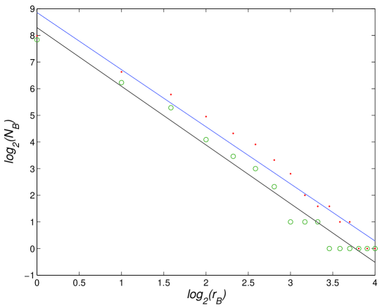
As an example, we used the above algorithm to estimate the fractal dimension of the human protein-protein interaction network as well as that of its skeleton. The result is shown in Fig. 1. When we applied the box covering algorithm on the skeleton, more boxes were needed for each fixed box radius . The increasing rate of the number of boxes varies when the size of the box increases. More specifically, when is smaller, the number of boxes needed is not much different for both the original network and its skeleton; but when is larger, many more boxes are needed to cover the skeleton than the original network.
2.2 Algorithms for multifractal analysis of networks
Real-world fractals may not be homogeneous; there is rarely an identical motif repeated on all scales. Two objects might have the same fractal dimension and yet look completely different. Real-world fractals possess rich scaling and self-similarity properties that can change from point to point, thus can have different dimensions at different scales. The present paper investigates these properties on complex networks, we aim to develop an approach for multifractal analysis of complex networks.
The most common algorithm of multifractal analysis is the fixed-size box-counting algorithm. For a given probability measure with support set in a metric space, we consider the partition sum
| (1) |
where is a real number and the sum runs over all different non-overlapping boxes of a given size in a covering of the support . It follows that and The mass exponent function of the measure is defined by
| (2) |
The generalized fractal dimensions of the measure are defined as
| (3) |
and
| (4) |
for , where .
For every box size , the number also referred to as the Hölder exponent, is the singularity strength of the box. This exponent may be interpreted as a crowding index of a measure of concentration: the greater is, the smaller is the concentration of the measure, and vice versa. For every box size , the numbers of cells in which the Hölder exponent has a value within the range behave like
The function signifies the Hausdorff dimension of the subset which has singularity ; that is, characterizes the abundance of cells with Hölder exponent and is called the singularity spectrum of the measure. The measure is said to be a multifractal measure if its singularity spectrum for a range of values of . The singularity spectrum and the mass exponent function are connected via the Legendre transform:
| (5) |
and
Considering the relationship between the mass exponent function and the generalized dimension function , the singularity spectrum contains exactly the same information as and .
The generalized fractal dimensions are estimated through a linear regression of against for , and similarly through a linear regression of against for . The value is called the information dimension and the correlation dimension.
For a network, the measure of each box is defined as the ratio of the number of nodes covered by the box and the total number of nodes in the network. The fixed-size box-counting algorithm of Ref. [14] described above could not be used to analyze the multifractal behavior of networks directly. Because the method contains a random process of selecting the position of the center of each box, this will affect the number of boxes with a fixed size. Especially, if a node with large degree (a hub) is randomly chosen, a lot more nodes could be covered, and it is an efficient way when we produce box covering. However, if a node with small degree is randomly chosen first, few nodes could be covered. As a result, the partition sum defined by Eq. (1) will change each time we proceed with box counting. To avoid this effect, we propose to take the average of the partition sums over a large number of times and accordingly modify the original fixed-size box-counting algorithm into a new method. To our knowledge, this improvement is the first introduced in this approach to analyze the multifractal behavior of complex networks.
We need to calculate the shortest-path distance matrix for each network and these matrices are the input data for fractal and multifractal analyses. We describe the procedure as follows:
-
(i)
Transform the pairs of edges and nodes in a network into a matrix , where is the number of nodes of the network. The matrix is a symmetric matrix where the elements or with when there is an edge between node and node , while when there is no edge between them. We define that each node has no edge with itself and accordingly .
Remark: could be the input data for calculating the degree distribution and characteristic path length to determine whether the network possesses the properties of scale-free degree distribution and small-world effect.
-
(ii)
Compute the shortest path length among all the linked pairs and save these pairs into another matrix .
Remark: In graph theory, calculation of the shortest path is a significant problem and there are many algorithms for solving this problem. Here, in our approach, we use Dijkstra’s algorithm of the Matlab toolbox.
After the above steps we could use the matrix as input data for multifractal analysis based on our modified fixed-size box counting algorithm as follows:
-
(i)
Initially, all the nodes in the network are marked as uncovered and no node has been chosen as a seed or center of a box.
-
(ii)
According to the number of nodes in the network, set appropriately. Group the nodes into different ordered random sequences. More specifically, in each sequence, nodes which will be chosen as seed or center of a box are randomly arrayed.
Remark: is the number of random sequences and is also the value over which we take the average of the partition sum . Here in our study, we set for all the networks in order to compare them. -
(iii)
Set the size of the box in the range , where is the diameter of the network.
Remark: When , the nodes covered within the same box must be connected to each other directly. When , the entire network could be covered in only one box no matter which node was chosen as the center of the box. -
(iv)
For each center of a box, search all the neighbors within distance and cover all nodes which are found but have not been covered yet.
-
(v)
If no newly covered nodes have been found, then this box is discarded.
-
(vi)
For the nonempty boxes , we define their measure as where is the number of nodes covered by the box , and is the number of nodes of the entire network.
-
(vii)
Repeat (iv) until all nodes are assigned to their respective boxes.
-
(viii)
When the process of box counting is finished, we calculate the partition sum as for each value of .
-
(ix)
Repeat (iii) and (iv) for all the random sequences, and take the average of the partition sums and then use for linear regression.
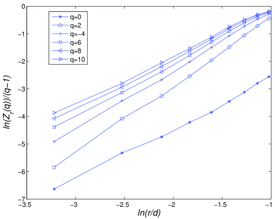
Linear regression is an essential step to get the appropriate range of and to get the generalized fractal dimensions . In our approach, we run the linear regression of against for , and similarly the linear regression of against for , where and is the diameter of the network. An example of linear regression for the Arabidopsis thaliana PPI network is shown in Fig. 2. The numerical results show that the best fit occurs in the range , hence we select this range to perform multifractal analysis and get the spectrum of generalized dimensions .
After this spectrum has been obtained, we use to verify how changes along each curve. The quantity has been used in the literature to describe the density of an object. In this paper, based on our modified fixed-size box covering method, can help to understand how the edge density changes in the complex network. In other words, a larger value of means the edge distribution is more uneven. More specifically, for a network, edge distribution could vary from an area of hubs where edges are dense to an area where nodes are just connected with a few links.
In the following sections, we calculate the generalized fractal dimensions . From the shape of , we determine the multifractality of the network using the method described above. We then calculate to verify how changes along each curve.
3 Results and discussions
In recent years, with the development of technology, the research on networks has shifted away from the analysis of single small graphs and the properties of individual vertices or edges within such graphs to consideration of large-scale statistical properties of complex networks. Newman reviewed some latest works on the structure and function of networked systems such as the Internet, the World Wide Web, social networks and a variety of biological networks. Besides reviewing empirical studies, the author also focused on a number of statistical properties of networks including path lengths, degree distributions, clustering and resilience. In this paper, we pay attention to another aspect of networks, namely their multifractality. We aim to develop a tool based on this property to characterize and classify real-world networks.
It has been shown that many real complex networks share distinctive characteristics that differ in many ways from random and regular networks. Fundamental properties of complex networks such small-world effect and the scale-free degree distribution have attracted much attention recently. These properties have in fact been found in many naturally occurring networks. In Subsections 3.1, 3.2 and 3.3, we generate scale-free networks using the BA model of Barabasi and Albert, small-world networks using the NW model of Newman and Watts, then random networks using the ER model of Erdös and Rényi respectively. We then apply our modified fixed-size box counting algorithm to analyze the multifractal behavior of these networks.
3.1 Scale-free networks
We use the elegant and simple BA model of Barabasi and Albert to generate scale-free networks. The origin of the scale-free behavior in many systems can be traced back to this BA model, which correctly predicts the emergence of scaling exponent. The BA model consists of two mechanisms : Initially, the network begins with a seed network of nodes, where and the degree of each node in the initial network should be at least 1, otherwise it will always remain disconnected from the rest of the network. For example, here we start with an initial network of 5 nodes. Its interaction matrix is
We then add one node to this initial network at a time. Each new node is connected to existing nodes with a probability that is proportional to the number of links that the existing nodes already have. Formally, the probability that the new node is connected to node is
| (6) |
where is the degree of node . So hubs tend to quickly accumulate even more links, while nodes with only a few links are unlikely to be chosen as destination for a new link.
In this paper, these scale-free networks are generated based on the same seed which is the initial network of 5 nodes. For better comparison, in each step, one node will be added into the network with one link. Then we apply the modified fixed-size box counting method on them to detect their multifractal behavior.
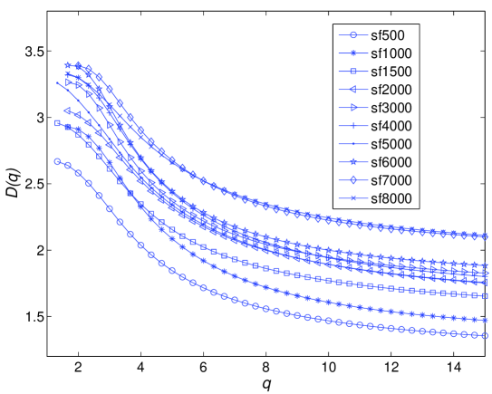
In Fig. 3. we can see that scale-free networks are multifractal by the shape of the curves. The functions of these networks decrease sharply after the peak. An explanation is that, in a scale-free network, there are several nodes which are known as hubs that have a large number of edges connected to them, so the edge density around the areas near the hubs is larger than the remaining parts of the network.
We summarize the numerical results in Table 1 including the number of nodes, number of edges, diameter, power law exponent , maximum value of , limit of , and . From these results we could see that scale free networks with larger size (more nodes and more edges) are likely to have larger values of the maximum and limit of . In other words, the function increases with the size of a scale-free network. An explanation for this situation is that larger scale-free networks usually have more hubs which make the structure of the network more complex.
Scale-free networks show a power-law degree distribution of , where is the probability of a node randomly chosen with degree . It was shown in Ref. [6, 7] that when the average degree diverges; while for the standard deviation of the degree diverges. It has been found that the degree exponent usually varies in the range of for most scale-free networks. Accordingly, we computed the power-law exponent of these generated scale-free networks. The results show that there doesn’t seem to be any clear relationship between power law and the maximum of limit of or .
3.2 Small-world networks
In 1998, Watts and Strogatz proposed a single-parameter small-world network model that bridges the gap between a regular network and a random graph. With the WS small-world model, one can link a regular lattice with pure random network by a semirandom network with high clustering coefficient and short average path length. Later on, Newman and Watts modified the original WS model. In the NW model, instead of rewiring links between nodes, extra links called shortcuts are added between pairs of nodes chosen at random, but no links are removed from the existing network. The NW model is equivalent to the WS model for small and sufficiently large , but easier to proceed.
In this paper, we use the NW model as follows. Firstly, we should select three parameters: the dimension , which is the number of nodes in a graph; the mean degree (assumed to be an even integer), which is the number of nearest-neighbors to connect; and the probability of adding a shortcut in a given row, where and . Secondly, we follow two steps:
-
(i)
Construct a regular ring lattice. For example, if the nodes are named , there is an edge between node and if and only if for ;
-
(ii)
Add a new edge between nodes and with probability .
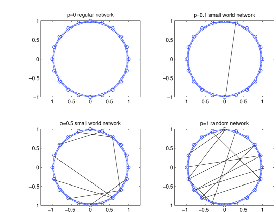
An illustration of this generating process is given in Fig. 4. The upper left figure corresponds to the probability . It is a regular network containing 20 nodes and each node has two neighbors on both sides. In other words, in this regular network, each node has four edges. Then we start generating small-world networks based on this regular network. The upper right figure of Fig. 4 corresponds to the probability one edge is added into the network. The network then becomes a small-world network. The bottom left figure corresponds to the probability seven edges are added into the original regular network and it is also a small-world network. The bottom right figure corresponds to the probability ; 10 edges are added into the original small-world network and this time it becomes a random network.
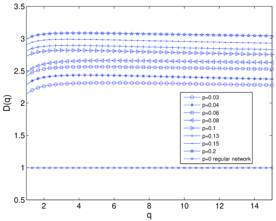
In this paper, we firstly generated a regular network which contains 5000 nodes and 250,000 edges. Each node has 50 edges on each side. Then we apply the modified fixed-size box counting method on this regular network. The numerical results are shown in the last row of Table 2. Both the maximum value of and the limit of are equal to one, thus . This is because regular networks are not fractal, and they have dimension one. Secondly, for better comparison, we generated ten small-world networks based on a regular network of 5000 nodes with 5 edges on each side of a node. During the generation, when the probability increases, more edges are added into the original regular network. Then we apply the modified fixed-size box counting method on them to detect their multifractal behavior. We summarize the numerical results in Table 2, which includes the number of nodes, number of edges, diameter, probability (the generating parameter), maximum value of and . These results indicate that, when increases, more edges are added and accordingly both the maximum and limit values of increase.
In Fig. 5 we can see that the curve of a regular network whose probability during generation is a straight line with the value of . The curves of the other small-world networks are also approximately straight lines but with different values. So these networks are not multifractal. Another interesting property is apparent when , in which case increases along with the value of . More specifically, when increases, more edges are added to the network, and both the maximum and limit values of and limit of increase. The values of are all within the error range, confirming that the curves are straight lines.
3.3 Random networks
The Erdös-Rényi random graph model is the oldest and one of the most studied techniques to generate complex networks.
We generate random networks based on the ER model:
-
(i)
Start with isolated nodes;
-
(ii)
Pick up every pair of nodes and connect them by an edge with probability
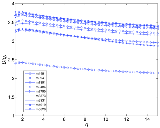
Usually, the results of this generation are separated subnetworks. In this work, we just consider the largest connected part as the network to work on and apply the modified fixed-size box counting method to detect their multifractal behaviors. We then summarize the numerical results in Table 3 including the number of nodes, number of edges, diameter, probability (the generating parameter), maximum value of , limit of , and . These results indicate that there is no clear relationship between and the size of the random network.
In Fig. 6, we can see that the curves of random networks decrease slowly after the peak and the changes could be seen by the values of . This pattern occurs because, during the generating process, nodes are randomly connected with probability , and few hubs may exist. Compared with scale-free networks, this decrease supports the claim that, in random networks, edges are distributed more symmetrically.
Remark: In the present study, we consider the generalized fractal dimensions to determine whether the object is multifactal from the shape of . For a monofractal system, which has the same scaling behavior at any point, should be a constant independent of , while for a multifractal, the should be a non-increasing nonlinear curve as increases. However, in our results, an anomalous behavior is observed: the curves increase at the beginning when . This anomalous behavior has also been observed in Bos et al., Smith and Lange, Fernández et al.. Some reasons for this behavior have been suggested, including that the boxes contain few elements, or the small scaling regime covers less than a decade so that we cannot extrapolate the box counting results for the partition function to zero box size. In encountering the anomalous spectra of , we tried another method of multifractal analysis called the sand-box method, but the linear regression fittings are not satisfactory. We therefore used the modified fixed-size box counting algorithm in this research. For the purpose of detecting the multifractality of complex networks, we adopt the anomalous spectra of and focus on the decreasing parts which are presented in Figs. 3 to 7.
3.4 Protein-protein interaction networks
Our fractal and multifractal analyses are based on connected networks which do not have separated parts or isolated nodes. In order to apply them to protein-protein interaction (PPI) networks, some preparation is needed in advance. Firstly, we need to find the largest connected part of each data set. For this purpose many tools and methods could be used. In our study, we adopt the Cytoscape which is an open bioinformatics software platform for visualizing molecular interaction networks and analyzing network graphs of any kind involving nodes and edges. In using Cytoscape, we could get the largest connected part of each interacting PPI data set and this connected part is the network on which fractal and multifractal analyses are performed.
The protein-protein interaction data we used here are mainly downloaded from two databases: The PPI networks of Drosophila melanogaster (fruit fly), C. elegans, Arabidopsis thaliana and Schizosaccharomyces pombe are downloaded from BioGRID. The PPI networks of S. cerevisiae (baker’s yeast), E. coli and H. pylori are download from DIP. We also use the same human PPI network data as in Ref. [55].
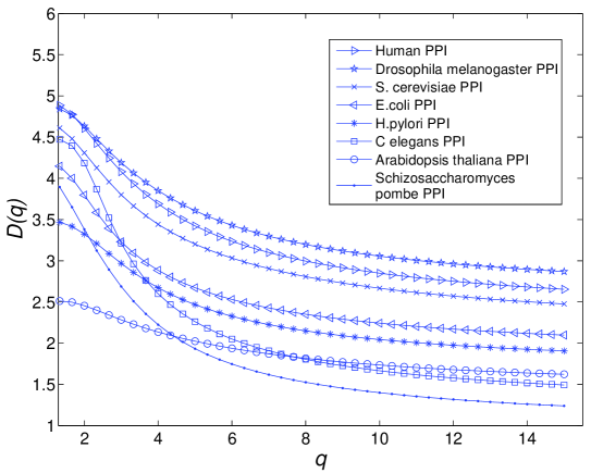
We calculated the spectra for eight PPI networks of different organisms as shown in Fig. 7. From these curves, we see that all PPI networks are multifractal and there are two clear groupings of organisms based on the peak values of their curves. The first group includes human, Drosophila melanogaster, S. cerevisiae, and C. elegans. The second group just includes two bacteria E.coli and H. pylori. We also see that the PPI networks of the eight organisms have similar shape for the curves. They all increase when , and reach their peak values around , then decrease sharply as and finally reach their limit value when . So we can take and use to verify how the function changes along each curve. We summarize the corresponding numerical results in Table 4.
4 Conclusions
After analyzing a variety of real complex networks, Song et al. found that they consist of self-repeating patterns on all length scales, i.e., complex networks have self-similar structures. They found that the box-counting method is a proper tool to unfold the self-similar properties of complex networks and to further investigate network properties.
However, describing objects by a single fractal dimension is a limitation of fractal analysis, especially when the networks exhibit a multifractal behavior. Multifractal analysis is a useful way to characterize the spatial heterogeneity of both theoretical and experimental fractal patterns. It allows the computation of a set of fractal dimensions, especially the generalized fractal dimensions .
A modified algorithm for analyzing the multifractal behavior of complex networks is introduced in this paper. This algorithm is applied on generated scale-free networks, small-world networks and random networks as well as protein-protein interaction networks. The numerical results indicate that multifractality exists in scale-free networks and PPI networks, while for small-world networks and random networks their multifractality is not clear-cut, particularly for small-world networks generated by the NW model. Furthermore, for scale-free networks, the values of increase when the size of the network increases because larger scale-free networks usually have more hubs which make the structure of the network more complex. However, for random networks there is no clear relationship between and the size of the network. The quantity has been used to investigate how changes. Larger means the network’s edge distribution is more uneven; while smaller means the network’s edge distribution is more symmetrical, which is the case for random networks.
These results support that the algorithm proposed in this paper is a suitable and effective tool to perform multifractal analysis of complex networks. Especially, in conjunction with the derived quantities from , the method and algorithm provide a needed tool to cluster and classify real networks such as the protein-protein interaction networks of organisms.
Acknowledgements
This project was supported by the Australian Research Council (Grant No. DP0559807), the Natural Science Foundation of China (Grant No. 11071282), the Chinese Program for Changjiang Scholars and Innovative Research Team in University (PCSIRT) (Grant No. IRT1179), the Chinese Program for New Century Excellent Talents in University (Grant No. NCET-08-06867), the Research Foundation of Education Commission of Hunan Province of China (grant No. 11A122), Hunan Provincial Natural Science Foundation of China (Grant No. 10JJ7001), Science and Technology Planning Project of Hunan province of China (Grant No. 2011FJ2011), the Lotus Scholars Program of Hunan province of China, the Aid Program for Science and Technology Innovative Research Team in Higher Education Institutions of Hunan Province of China, and a China Scholarship Council–Queensland University of Technology Joint Scholarship.
References
- [1]
- [1] Song C, Havlin S and Makse H A, 2005 Nature 433 392
- [2] Lee C Y and Jung S 2006 Phys. Rev. E 73 066102
- [3] Guo L and Cai X 2009 Chin. Phys. Lett. 26 088901
- [4] Erdos P and Renyi A 1960 Publ. Math. Inst. Hung. Acad. Sci. 5 17
- [5] Milgram S 1967 Psychol. Today 2 60
- [6] Albert R, Jeong H and Barabasi A L 1999 Nature 401 130
- [7] Albert R and Barabasi A L 2002 Rev. Mod. Phys. 74 47
- [8] Faloutsos M, Faloutsos P and Faloutsos C 1999 Comput. Commun. Rev. 29 251
- [9] Mandelbrot B B 1983 The fractal Geometry of Nature (New York, Academic Press)
- [10] Feder J 1988 Fractals (New York, Plenum)
- [11] Falconer K 1997 Techniques in Fractal Geometry (New York, Wiley)
- [12] Eguiluz V M, Hernandez-Garcia E, Piro O and Klemm K 2003 Phys. Rev. E 68 055102(R)
- [13] Song C, Gallos L K, Havlin S and Makse H A 2007 J. Stat. Mech.: Theor. Exper. 3 P03006
- [14] Kim J S, Goh K I, Salvi G, Oh E, Kahng B, and Kim D 2007 Phys. Rev. E 75 016110
- [15] Zhou W X, Jiang Z Q and Sornette D 2007 Physica A 375 741
- [16] Gao L, Hu Y and Di Z 2008 Phys. Rev. E 78 046109
- [17] Shanker O 2007 Mod. Phys. Lett.B 21 321
- [18] Rozenfeld H D and Makse H A 2009 Chem. Engneer. Sci. 64 4572
- [19] Rozenfeld H D, Song C and Makse H A 2010 Phys. Rev. Lett. 104 025701
- [20] Liu J X and Kong X M 2010 Acta Physica Sinica 59(4) 2244
- [21] Grassberger P and Procaccia I 1983 Phys. Rev. Lett. 50 346
- [22] Halsey T C, Jensen M H, Kadanoff L P, Procaccia I, and Shraiman B I 1986 Phys. Rev. A 33 1141
- [23] Canessa E 2000 J. Phys. A: Math. Gen. 33 3637
- [24] Anh V V, Tieng Q M and Tse Y K 2000 Int. Trans. Oper. Res. 7 349
- [25] Yu Z G, Anh V and Lau K S 2001 Physica A 301 351
- [26] Yu Z G, Anh V and Lau K S 2001 Phys. Rev. E 64 31903
- [27] Yu Z G, Anh V and Wang B 2001 Phys. Rev. E 63 11903
- [28] Anh V, Lau K S and Yu Z G 2002 Phys. Rev. E 66 031910
- [29] Yu Z G, Anh V and Lau K S 2003 Phys. Rev. E 68 021913
- [30] Yu Z G, Anh V and Lau K S 2004 J. Theor. Biol. 226 341
- [31] Zhou L Q, Yu Z G, Deng J Q, Anh V and Long S C 2005 J. Theor. Biol. 232 559
- [32] Yu Z G, Anh V, Lau K S and Zhou L Q 2006 Phys. Rev. E 73 031920
- [33] Yu Z G, Xiao Q J, Shi L, Yu J W, and Anh V 2010 Chin. Phys. B 19 (6) 068701
- [34] Zhu S M, Yu Z G, Anh V 2011 Chin. Phys. B 20 (1) 010505
- [35] Han J J and Fu W J 2010 Chin. Phys. B 19 (1) 010205
- [36] Kantelhardt J W, Koscielny-Bunde E, Rybski D, Braun P, Bunde A and Havlin S 2006 J. Geophys. Res. 111 D01106
- [37] Veneziano D, Langousis A and Furcolo P 2006 Water Resour. Res. 42 W06D15
- [38] Venugopal V, Roux S G, Foufoula-Georgiou E and Arneodo A 2006 Water Resour. Res. 42 W06D14
- [39] Yu Z G, Anh V, Wanliss J A and Watson S M 2007 Chaos, Solitons and Fractals 31 736
- [40] Zang B J and Shang P J 2007 Chin. Phys. 16 (3) 565
- [41] Yu Z G, Anh V and Eastes R 2009 J. Geophys. Res. 114 A05214
- [42] Yu Z G, Anh V, Wang Y, Mao D and Wanliss J 2010 J. Geophys. Res. 115 A10219
- [43] Polla G, Lovasz L and Vicsek T 2010 Proc. Natl. Acad. Sci. U.S.A. 107 7640
- [44] Dijkstra E W 1959 Numerische Mathematik 1 269
- [45] Newman M E J 2003 SIAM Rev. 45 167
- [46] Barabsi A L and Albert R 1999 Science 286 509
- [47] Newman M E J and Watts D J 1999 Phys. Lett. A 263 341
- [48] Watts D J and Strogatz S H 1998 Nature 393 440
- [49] Opheusden J H H, Bos M T A, and van der Kaaden G 1996 Physica A 227 183
- [50] Smith T G and Lange G D 1998 in Fractal in Biology and Medicine (Eds: Nonnenmacher T F, Losa G A and Weibel E R) (Basel, Birkhäuser)
- [51] Fernndez E, Bolea J A, Ortega G and Louis E 1999 J. Neurosci. Methods 89 151
- [52] Cytoscape software: http://cytoscapeweb.cytoscape.org/
- [53] BioGRID: http://thebiogrid.org/download.php
- [54] DIP: http://dip.doe-mbi.ucla.edu/dip/Download.cgi
- [55] Lee E, Jung H, Radivojac P, Kim J W and Lee D 2009 BMC Bioinformatics 10 (Suppl 2) S2
| Number of nodes | Number of edges | Diameter | Max(Dq) | Lim(Dq) | ||
|---|---|---|---|---|---|---|
| 500 | 499 | 13 | 1.94 0.02 | 2.67 | 1.36 | 1.31 |
| 1000 | 999 | 16 | 2.02 0.07 | 2.93 | 1.47 | 1.46 |
| 1500 | 1499 | 17 | 2.09 0.04 | 2.96 | 1.65 | 1.30 |
| 2000 | 1999 | 20 | 1.99 0.08 | 3.05 | 1.76 | 1.29 |
| 3000 | 2999 | 20 | 2.06 0.04 | 3.26 | 1.83 | 1.44 |
| 4000 | 3999 | 23 | 2.09 0.03 | 3.32 | 1.80 | 1.52 |
| 5000 | 4999 | 23 | 2.08 0.04 | 3.26 | 1.75 | 1.51 |
| 6000 | 5999 | 22 | 2.06 0.04 | 3.39 | 1.88 | 1.51 |
| 7000 | 5999 | 28 | 2.08 0.04 | 3.39 | 2.10 | 1.29 |
| 8000 | 5999 | 25 | 1.91 0.12 | 3.33 | 2.11 | 1.22 |
| Number of nodes | Number of edges | Diameter | p | Max(Dq) | Lim(Dq) | |
|---|---|---|---|---|---|---|
| 5000 | 25159 | 33 | 0.03 | 2.31 | 2.28 | 0.03 |
| 5000 | 25207 | 29 | 0.04 | 2.43 | 2.37 | 0.06 |
| 5000 | 25290 | 23 | 0.06 | 2.56 | 2.53 | 0.03 |
| 5000 | 25358 | 23 | 0.08 | 2.66 | 2.63 | 0.03 |
| 5000 | 25513 | 18 | 0.1 | 2.81 | 2.75 | 0.06 |
| 5000 | 25621 | 15 | 0.13 | 2.89 | 2.83 | 0.06 |
| 5000 | 25792 | 15 | 0.15 | 2.99 | 2.93 | 0.06 |
| 5000 | 26017 | 12 | 0.2 | 3.08 | 3.04 | 0.04 |
| regular network 5000 | 250000 | 50 | 0 | 1 | 1 | 0.00 |
| Number of nodes | Number of edges | Diameter | p | Max(Dq) | Lim(Dq) | |
|---|---|---|---|---|---|---|
| 449 | 610 | 15 | 0.005 | 2.42 | 2.14 | 0.28 |
| 994 | 2502 | 8 | 0.005 | 3.32 | 2.87 | 0.45 |
| 1991 | 5939 | 9 | 0.003 | 3.73 | 3.41 | 0.32 |
| 2484 | 6310 | 11 | 0.002 | 3.70 | 3.33 | 0.37 |
| 2790 | 4374 | 18 | 0.001 | 3.29 | 2.95 | 0.34 |
| 3373 | 5978 | 15 | 0.001 | 3.47 | 3.15 | 0.32 |
| 3931 | 8125 | 13 | 0.001 | 3.67 | 3.35 | 0.31 |
| 4919 | 10179 | 13 | 0.0008 | 3.78 | 3.39 | 0.39 |
| 5620 | 8804 | 16 | 0.00058 | 3.54 | 3.21 | 0.33 |
| Networks | Number of nodes | Number of edges | Diameter | Max(Dq) | Lim(Dq) | ||
|---|---|---|---|---|---|---|---|
| Human | 8934 | 41341 | 14 | 2.34 | 4.89 | 2.65 | 2.24 |
| Drosophila Melanogaster | 7476 | 26534 | 11 | 2.34 | 4.84 | 2.87 | 1.97 |
| S. cerevisiae | 4976 | 21875 | 10 | 2.36 | 4.62 | 2.48 | 2.14 |
| E.coli | 2516 | 11465 | 12 | 2.14 | 4.15 | 2.10 | 2.05 |
| H.pylori | 686 | 1351 | 9 | 2.27 | 3.47 | 1.91 | 1.56 |
| C.elegans | 3343 | 6437 | 13 | 2.28 | 4.47 | 1.49 | 2.98 |
| Arabidopsis Thaliana | 1298 | 2767 | 25 | 1.83 | 2.51 | 1.62 | 0.89 |
