Diffusion model for the time evolution of particle loss rates in collimator scans: a method for measuring stochastic transverse beam dynamics
in circular accelerators

Abstract

A diffusion model of the time evolution of loss rates caused by a step in collimator position is presented. It builds upon the model of Ref. Seidel:1994 and its assumptions: (1) constant diffusion rate within the range of the step and (2) linear halo tails. These hypotheses allow one to obtain analytical expressions for the solutions of the diffusion equation and for the corresponding loss rates vs. time. The present model addresses some of the limitiations of the previous model and expands it in the following ways: (a) losses before, during, and after the step are predicted; (b) different steady-state rates before and after are explained; (c) determination of the model parameters (diffusion coefficient, tail population, detector calibration, and background rate) is more robust and precise. These calculations are the basis for the measurement of transverse beam diffusion rates as a function of particle amplitude with collimator scans. The results of these measurements in the Tevatron will be presented in a separate report.

I Introduction

Figure 1: Example of loss rate data taken during a collimator scan in Tevatron Store 8749 (20 May 2011): local loss rate (top, device T:LF480); collimator position (bottom, device T:F48VCP). The collimator steps take about 0.2 s. In this example the collimator position was recorded only every 15 s.

Phenomena related to the stochastic transverse beam dynamics in circular accelerators can be described in terms of particle diffusion Lichtenberg:1992 ; Chen:PRL:1992 ; Gerasimov:FERMILAB:1992 ; Zimmermann:PA:1994 ; Sen:PRL:1996 . It was demonstrated that these effects can be observed with collimator scans Seidel:1994 . Usually, collimator jaws are the devices that are closest to the beam and they define the machine aperture. If they are moved towards the beam center in small steps, typical spikes in the local shower rate are observed, which approach a new steady-state level with a characteristic relaxation time. When collimators are retracted, on the other hand, a dip in losses is observed, which also tends to a new equilibrium level (Figure 1). A detailed description of the Tevatron collimation system can be found in Ref. Mokhov:JINST:2011 .

These phenomena have been used to estimate the diffusion rate in the beam halo in the SPS at CERN Burnod:CERN:1990 , in HERA at DESY Seidel:1994 , and in RHIC at BNL Fliller:PAC:2003 . Similar measurements were carried out at the Tevatron in 2011. Besides the interest in characterizing the beam dynamics of colliding beams, these measurements were motivated by the study of the effects of the novel hollow electron beam collimator Stancari:PRL:2011 .

Here we present a more complete model of beam evolution under diffusion. It will serve as the basis for interpreting of Tevatron data. Previous models are extended to explain the behavior of losses before, during, and after the collimator step. This allows one to extract the diffusion rate in a more robust way, by taking into account not only the relaxation time, but also the steady-state loss rates before and after the step and the peak or dip value. The analysis of Tevatron data will be presented in a separate report. This model can also be applied to the dynamics of beams in the LHC.

II Model

Following Ref. Seidel:1994 , we consider the evolution in time $t$ of a beam of particles with phase-space density $f(J,t)$ described by the diffusion equation:

$$\partial_{t}f=\partial_{J}\left(D\,\partial_{J}f\right)$$ (1)

where $J$ is the Hamiltonian action and $D(J)$ the diffusion coefficient. The particle flux at a given location $J=J^{\prime}$ is $\phi=-D\cdot\left[\partial_{J}f\right]_{J=J^{\prime}}$.

During a collimator step, the action $J_{c}=x^{2}_{c}/\beta_{c}$, corresponding to the collimator position $x_{c}$ at a ring location where the amplitude function is $\beta_{c}$, changes from its initial value $J_{ci}$ to its final value $J_{cf}$ during a time $\Delta t$. The step in action is $\Delta J\equiv J_{cf}-J_{ci}$. In the Tevatron, typical steps are $50\ \mathrm{\mu m}$ in 0.2 s, and the amplitude function is tens of meters. The behavior of $J_{c}(t)$ can be modeled, for instance, by a linear function connecting $J_{ci}$ with $J_{cf}$:

$$J_{c}(t)=\left\{\begin{array}[]{ll}J_{ci}&t\leq 0\\ J_{ci}+(J_{cf}-J_{ci})\cdot t/\Delta t&0<t<\Delta t\\ J_{cf}&\Delta t\leq t\end{array}\right.$$ (2)

It is assumed that the collimator steps are small enough so that the diffusion coefficient can be treated as a constant in that region. This hypothesis is justified by the fact that the fractional change in action is of the order of $\Delta J_{c}/J_{c}\sim(2)(25\ \mathrm{\mu m})/(2\ \mathrm{mm})=2.5\%$. Because the diffusion coefficient is a strong function of action ($D\sim J^{4}$), this translates into a variation of 10% in the diffusion rate, an acceptable systematic in a quantity that varies by orders of magnitude. If $D$ is constant, the diffusion equation becomes

$$\partial_{t}f=D\,\partial_{JJ}f.$$ (3)

With these definitions, the particle loss rate at the collimator is

$$L=-D\cdot\left[\partial_{J}f\right]_{J=Jc}.$$ (4)

Particle showers caused by the loss of beam are measured with scintillator counters placed close to the collimator jaw. The observed shower rate is parameterized as follows

$$S=kL+B,$$ (5)

where $k$ is a normalization constant including detector acceptance and efficiency and $B$ is a background term which includes, for instance, the effect of residual activation. Both $k$ and $B$ are assumed to be independent of collimator position and time during the scan.

III Boundary conditions

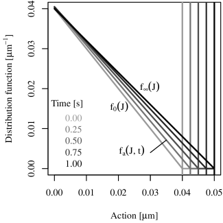
Figure 2: Illustration of boundary conditions in the case of an outward collimator step: initial distribution $f_{0}(J)$, intermediate asymptotic distributions $f_{a}(J,t)$, final distribution $f_{\infty}(J)$. The vertical lines represent the positions of the collimator vs. time. Parameters in this example are $J_{ci}=0.04\ \mathrm{\mu m}$, $J_{cf}=0.05\ \mathrm{\mu m}$, $A_{i}=1\ \mathrm{\mu m^{-2}}$, $A_{f}=0.8\ \mathrm{\mu m^{-2}}$, $\Delta t=1\ \mathrm{s}$.

The collimator is treated as a perfect absorber, so that the boundary condition for the phase-space density becomes

$$f(J,t)=0\ \ \ \mbox{for $J\geq J_{c}$}.$$ (6)

We assume that cancellation of the particle flux at $J=0$ is automatically satisfied by $D(0)\simeq 0$, so no boundary condition is imposed there. This greatly simplifies the form of Green’s function (see below).

As initial conditions and asymptotic behavior for the phase-space density we use linear functions of action:

$$f_{0}(J)\equiv f(J,0)=\left\{\begin{array}[]{ll}(J_{ci}-J)\cdot A_{i}&J<J_{ci}\\ 0&J_{ci}\leq J\end{array}\right.$$ (7)

$$f_{\infty}(J)=f(J,\infty)=\left\{\begin{array}[]{ll}(J_{cf}-J)\cdot A_{f}&J<J_{cf}\\ 0&J_{cf}\leq J\end{array}\right.,$$ (8)

where $A_{i}$ and $A_{f}$ are constants. This is the essential hypothesis that allows one to obtain analytical solutions for the time evolution of the distribution function. It is justified by considering these expressions as the first term in the Taylor expansion of the beam tails. A linear behavior of the asymptotic solution also gives a constant steady-state flux.

In this respect, the present model differs from that of Ref. Seidel:1994 . We allow the slopes of the initial and final distributions to be different. This is necessary to explain the difference in the steady-state loss rates $L$ before and after the collimator step. If one assumes the same diffusion coefficient and the same slope before and after, then one can only predict the same steady-state rate. Including the measured steady-state loss rates before and after the collimator step helps to disentangle the effects of population and diffusion, and to give a physical meaning to the model parameters.

Because of its linearity, a solution of the diffusion equation can be found using the method of Green’s functions:

$$f(J,t)=f_{a}+\int_{0}^{J_{c}}\left(f_{0}-f_{a}\right)\cdot G(J,J^{\prime},t)\,dJ^{\prime},$$ (9)

where $G(J,J^{\prime},t)$ is Green’s function for the given problem, $f_{0}$ (Eq. 7) is the initial distribution, and $f_{a}$ is an asymptotic solution. We are looking for a model of losses not only before and after the collimator step, but also as the collimator is moving. In this respect, too, this model extends that of Ref. Seidel:1994 . For this reason, we use $f_{a}=f_{\infty}$ (Eq. 8) for $J_{c}=J_{cf}$ (i.e., $t\geq\Delta t$) and

$$f_{a}(J,t)=\left\{\begin{array}[]{ll}(J_{c}-J)\cdot A_{c}&J<J_{c}\\ 0&J_{c}\leq J\end{array}\right.,$$ (10)

as the collimator moves ($0<t<\Delta t$). The parameter $A_{c}(t)$ is chosen to vary linearly between $A_{i}$ and $A_{f}$,

$$A_{c}(t)=\left\{\begin{array}[]{ll}A_{i}&t\leq 0\\ A_{i}+(A_{c}-A_{i})\cdot t/\Delta t&0<t<\Delta t\\ A_{f}&\Delta t\leq t\end{array}\right.,$$ (11)

so that the asymptotic solution transitions smoothly from Eq. 7 to Eq. 8. The initial and asymptotic solutions are illustrated in Figure 2.

The basic kernel for the diffusion equation is

$$K(J,J^{\prime},t)=\frac{1}{\sqrt{2\pi}\sigma}\exp{\left[-\frac{1}{2}\left(\frac{J-J^{\prime}}{\sigma}\right)^{2}\right]},$$ (12)

with $\sigma\equiv\sqrt{2Dt}$. To satisfy the boudary condition at the collimator (Eq. 6), an antisymmetric Green’s function can be used:

$$G(J,J^{\prime},t) = \left\{\exp{\left[-\frac{1}{2}\left(\frac{(J_{c}-J^{\prime})-(J_{c}-J)}{\sigma}\right)^{2}\right]}-\exp{\left[-\frac{1}{2}\left(\frac{(J_{c}-J^{\prime})+(J_{c}-J)}{\sigma}\right)^{2}\right]}\right\},$$ (13)

$$\cdot\frac{1}{\sqrt{2\pi}\sigma}$$

so that

$$G(J=J_{c},J^{\prime},t)=G(J,J^{\prime}=J_{c},t)=0.$$ (14)

The requirement that the solution be zero beyond the collimator position,

$$G(J,J^{\prime},t)=0\ \ \ \mbox{if $J_{c}<J$ or $J_{c}<J^{\prime}$},$$ (15)

is automatically satisfied by limiting the integration region between $0$ and $J_{c}$ (Eq. 9). Imposing additional boundary conditions at $J=0$ would require $G$ to be an infinite series. The analytical approximation used here does not constrain the phase-space density or its gradient at the origin, but it turns out a posteriori that $f(0,t)$ does not vary significantly if $f_{0}(0)\simeq f_{\infty}(0)$, which is what one would expect for a collimator step affecting the beam halo and not the beam core. Green’s function also satisfies the general symmetry property $G(J,J^{\prime},t)=G(J^{\prime},J,t)$. We also note its asymptotic behavior in time: $G(J,J^{\prime},0)=\delta(J-J^{\prime})$ and $G(J,J^{\prime},\infty)=0$, which justifies the physical interpretation of $f_{0}$ and $f_{a}$ in Eq. 9 as initial and asymtotic solutions.

IV Solutions

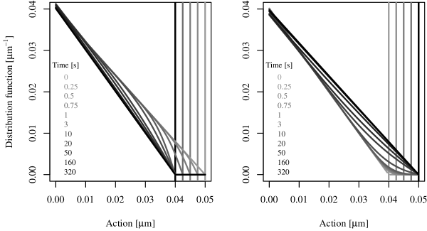
Figure 3: Evolution of distribution function during collimator step: $f_{I}(J,t)$ (inward, left) and $f_{O}(J,t)$ (outward, right). The vertical lines represent the positions of the collimator vs. time. Collimator action varies between $J_{ci}=0.05\ \mathrm{\mu m}$ and $J_{cf}=0.04\ \mathrm{\mu m}$ in the inward case (viceversa in the outward case) in a time $\Delta t=1\ \mathrm{s}$. The slopes of the tails are $A_{i}=0.8\ \mathrm{\mu m^{-2}}$ and $A_{f}=1\ \mathrm{\mu m^{-2}}$ in the inward case (viceversa outwards). The diffusion coefficient is $D=10^{-5}\ \mathrm{\mu m^{2}/s}$.

By setting up the diffusion model in the way described above, solutions can be expressed analytically through Eq. 9. It is convenient to treat the cases of inward ($J_{cf}<J_{ci}$) and outward ($J_{ci}<J_{cf}$) movement separately. In the inward case, the integrand is $f_{0}-f_{a}=A_{i}(J_{ci}-J)-A_{c}(J_{c}-J)$. In the outward case, it is convenient to divide the integral into two parts:

$$\int_{0}^{J_{c}}=\int_{0}^{J_{ci}}+\int_{J_{ci}}^{J_{c}}.$$ (16)

This is done because $f_{0}$ is null beyond the initial collimator position: $f_{0}-f_{a}=-f_{a}$ (see also Figure 2). To express the primitive of the Gaussian function, we use the cumulative Gaussian distribution function $P(x)$, defined in Appendix A. (Another possible choice is the so-called error function.) Integration yields the solutions of the diffusion equation in the two cases, $f_{I}(J,t)$ (inward step) and $f_{O}(J,t)$ (outward), subject to the boundary conditions specified above:

$$f_{I}(J,t)= - A_{i}(J_{ci}+J-2J_{c})$$

$$+ 2P\left(\frac{J_{c}-J}{\sigma}\right)A_{i}(J_{ci}-J_{c})$$

$$- P\left(\frac{-J}{\sigma}\right)\left[A_{i}(J_{ci}-J)-A_{c}(J_{c}-J)\right]$$

$$+ P\left(\frac{J-2J_{c}}{\sigma}\right)\left[A_{i}(J_{ci}+J-2J_{c})+A_{c}(J_{c}-J)\right]$$

$$+ \frac{\sigma}{\sqrt{2\pi}}(A_{c}-A_{i})\left\{\exp{\left[-\frac{1}{2}\left(\frac{J}{\sigma}\right)^{2}\right]}-\exp{\left[-\frac{1}{2}\left(\frac{J-2J_{c}}{\sigma}\right)^{2}\right]}\right\}$$

$$f_{O}(J,t)= + P\left(\frac{J_{ci}-J}{\sigma}\right)A_{i}(J_{ci}-J)$$

$$- 2P\left(\frac{J_{ci}+J-2J_{c}}{\sigma}\right)A_{i}(J_{ci}+J-2J_{c})$$

$$- P\left(\frac{-J}{\sigma}\right)\left[A_{i}(J_{ci}-J)-A_{c}(J_{c}-J)\right]$$

$$+ P\left(\frac{J-2J_{c}}{\sigma}\right)\left[A_{i}(J_{ci}+J-2J_{c})+A_{c}(J_{c}-J)\right]$$

$$+ \frac{\sigma}{\sqrt{2\pi}}A_{i}\left\{\exp{\left[-\frac{1}{2}\left(\frac{J_{ci}-J}{\sigma}\right)^{2}\right]}-\exp{\left[-\frac{1}{2}\left(\frac{J_{ci}+J-2J_{c}}{\sigma}\right)^{2}\right]}\right\}$$

$$+ \frac{\sigma}{\sqrt{2\pi}}(A_{c}-A_{i})\left\{\exp{\left[-\frac{1}{2}\left(\frac{J}{\sigma}\right)^{2}\right]}-\exp{\left[-\frac{1}{2}\left(\frac{J-2J_{c}}{\sigma}\right)^{2}\right]}\right\}$$

Some examples of the evolution of the phase-space density described by these functions are shown in Figure 3. A few representative snapshots in time are chosen: during collimator movement; a short time after the step, with a time scale determined by $t_{s}=\left|J_{ci}-J_{cf}\right|^{2}/D=10\ \mathrm{s}$; and a long time after the step, with a characteristic time $t_{l}=\left[\min{(J_{ci},J_{cf})}\right]^{2}/D=160\ \mathrm{s}$.

V Time evolution of losses

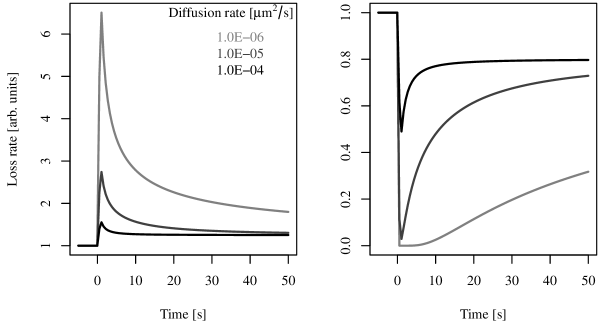
Figure 4: Calculated evolution of loss rates $L(t)$ during a collimator step according to Eqs. 4, V and V: inward (left) and outward (right). Collimator action varies between $J_{ci}=0.05\ \mathrm{\mu m}$ and $J_{cf}=0.04\ \mathrm{\mu m}$ in the inward case (viceversa in the outward case) in a time $\Delta t=1\ \mathrm{s}$ (see also Figure 3). The effect of 3 different values of the diffusion coefficient $D$ is shown. The slopes of the tails are scaled so that the initial and final steady-state loss rates are the same in all cases: $A_{i}=1/D$, $A_{f}=A_{i}J_{ci}/J_{cf}$.

Local losses are proportional to the gradient of the distribution function at the collimator (Eq. 4). The partial derivatives of the phase-space density with respect to action are the following:

$$\partial_{J}f_{I}(J,t)= - A_{i}+(A_{i}-A_{c})\left[P\left(\frac{-J}{\sigma}\right)+P\left(\frac{J-2J_{c}}{\sigma}\right)\right]$$

$$+ \frac{1}{\sqrt{2\pi}\sigma}\left\{2A_{i}(J_{c}-J_{ci})\exp{\left[-\frac{1}{2}\left(\frac{J_{c}-J}{\sigma}\right)^{2}\right]}+\right.$$

$$\left.(A_{i}J_{ci}-A_{c}J_{c})\left[\exp{\left[-\frac{1}{2}\left(\frac{J}{\sigma}\right)^{2}\right]}+\exp{\left[-\frac{1}{2}\left(\frac{J-2J_{c}}{\sigma}\right)^{2}\right]}\right]\right\},$$

$$\partial_{J}f_{O}(J,t)= - A_{i}\left[P\left(\frac{J_{ci}-J}{\sigma}\right)+P\left(\frac{J_{ci}+J-2J_{c}}{\sigma}\right)\right]$$

$$+ (A_{i}-A_{c})\left[P\left(\frac{-J}{\sigma}\right)+P\left(\frac{J-2J_{c}}{\sigma}\right)\right]$$

$$+ \frac{A_{i}J_{ci}-A_{c}J_{c}}{\sqrt{2\pi}\sigma}\left\{\exp{\left[-\frac{1}{2}\left(\frac{J}{\sigma}\right)^{2}\right]}+\exp{\left[-\frac{1}{2}\left(\frac{J-2J_{c}}{\sigma}\right)^{2}\right]}\right\}.$$

The value of the gradient at the collimator is therefore

$$\partial_{J}f_{I}(J_{c},t)= - A_{i}+2(A_{i}-A_{c})P\left(\frac{-J_{c}}{\sigma}\right)$$

$$+ \frac{1}{\sqrt{2\pi}\sigma}\left\{-2A_{i}(J_{ci}-J_{c})+2(A_{i}J_{ci}-A_{c}J_{c})\exp{\left[-\frac{1}{2}\left(\frac{J_{c}}{\sigma}\right)^{2}\right]}\right\},$$

$$\partial_{J}f_{O}(J_{c},t)= - 2A_{i}P\left(\frac{J_{ci}-J_{c}}{\sigma}\right)+2(A_{i}-A_{c})P\left(\frac{-J_{c}}{\sigma}\right)$$

$$+ 2\frac{A_{i}J_{ci}-A_{c}J_{c}}{\sqrt{2\pi}\sigma}\exp{\left[-\frac{1}{2}\left(\frac{J_{c}}{\sigma}\right)^{2}\right]}.$$

These are the functions that are used to model the measured shower rates (Eqs. 4 and 5). As expected, both functions tend to $-A_{i}$ for $t\to 0$ and to $-A_{f}$ as $t\to\infty$. For the $t\to 0$ limit to hold for the outward solution, it is necessary that $J_{c}\to J_{ci}$ faster than $\sqrt{t}$, which is satisfied by the linear approximation adopted here; otherwise, the slope will tend to zero.

These functions explain the data very well. In the transient region, after the collimator has reached its final position, they agree with those calculated in Ref. Seidel:1994 . Their main feature is a decay proportional to the square root of time (through the parameter $\sigma$), as is typical of diffusion processes. A few examples are plotted in Figure 4.

VI Comments on parameter estimation

Having a model that describes the data before, during, and after the collimator step has several advantages. The products $kDA_{i}+B$ and $kDA_{f}+B$ are determined by the steady-state loss rates. If a data set includes measurements of several steps at different amplitudes, the parameters $k$ and $B$, which are independent of $J$ and $t$, can be determined separately. Therefore, steady-state rates constrain the products $DA_{i}$ and $DA_{f}$ at each step.

The value of the diffusion coefficient $D$ is constrained both by the peak (or dip) value relative to the steady-state rate and by the duration of the transient through the parameter $\sigma$. In fact, the peak (or dip) value of the loss rate is achieved when the collimator reaches its final position ($J_{c}=J_{cf}$, $t=\Delta t$). At this point, neglecting the background, the loss rate is

$$S(\Delta t)\simeq kDA_{i}\left[1\pm\frac{\left|\Delta J\right|}{\sqrt{\pi\,D\,\Delta t}}\right],$$ (23)

whereas $S(0)\simeq kDA_{i}$. It follows that an estimate of the diffusion rate is

$$D\simeq\frac{(\Delta J)^{2}}{\pi\,\Delta t\,\left[S(\Delta t)/S(0)-1\right]^{2}}.$$ (24)

On the other hand, losses relax with a typical time constant that depends on the diffusion rate and on the magnitude of the step. One may define the characteristic time $t_{\pi}$ so that

$$\frac{\left|\Delta J\right|}{\sqrt{\pi\,D\,t_{\pi}}}\simeq\frac{1}{\sqrt{\pi}}=0.56,$$ (25)

meaning that the magnitude of the transient at time $t_{\pi}$ is about half of that of the steady-state rate. Therefore, we have an independent estimate of $D$:

$$D\simeq\frac{(\Delta J)^{2}}{t_{\pi}}.$$ (26)

If only the $t>\Delta t$ data is considered, as is done in Ref. Seidel:1994 , this is the only available information on $D$. In addition, in this case, the diffusion coefficient is highly correlated with the steady-state parameters.

These rough estimates of the model parameters can be used as initial guesses in a least-squares fit of the data.

Appendix A Useful formulas

To express the solutions of the diffusion equation, we use the cumulative Gaussian distribution function $P(x)$, defined as follows:

$$P(x)\equiv\frac{1}{\sqrt{2\pi}}\int_{-\infty}^{x}\exp{(-z^{2}/2)}\,dz.$$ (27)

Therefore, $P(-\infty)=0$, $P(0)=1/2$, and $P(\infty)=1$. By definition, the integral of a Gaussian function can be expressed as follows:

$$\frac{1}{\sqrt{2\pi}\sigma}\int_{z_{1}}^{z_{2}}\exp{\left[-\frac{1}{2}\left(\frac{z-z_{0}}{\sigma}\right)^{2}\right]}\,dz=P\left(\frac{z_{2}-z_{0}}{\sigma}\right)-P\left(\frac{z_{1}-z_{0}}{\sigma}\right).$$ (28)

For our purposes, another useful integral is

$$\frac{1}{\sqrt{2\pi}\sigma}\int_{z_{1}}^{z_{2}}z\,\exp{\left[-\frac{1}{2}\left(\frac{z-z_{0}}{\sigma}\right)^{2}\right]}\,dz=z_{0}\left[P\left(\frac{z_{2}-z_{0}}{\sigma}\right)-P\left(\frac{z_{1}-z_{0}}{\sigma}\right)\right]$$ (29)

$$-\frac{\sigma}{\sqrt{2\pi}}\left\{\exp{\left[-\frac{1}{2}\left(\frac{z_{2}-z_{0}}{\sigma}\right)^{2}\right]}-\exp{\left[-\frac{1}{2}\left(\frac{z_{1}-z_{0}}{\sigma}\right)^{2}\right]}\right\}.$$

Appendix B Scripts

Numerical calculations, data analysis, and graphics were done with the open-source, multi-platform statistical package R version 2.12.0 (2010-10-15) R . This documentation was produced by integrating LaTeX with R using the Sweave package. The source code can be found in the file dmcs.tar.gz. Below is the R part of the code.

[2]dmcs.R