Discrete spectra for confined and unconfined $-a/r+br^{2}$ potentials in $d$-dimensions

Abstract

Exact solutions to the $d$-dimensional Schrödinger equation, $d\geq 2$, for Coulomb plus harmonic oscillator potentials $V(r)=-a/r+br^{2}$, $b>0$ and $a\neq 0$ are obtained. The potential $V(r)$ is considered both in all space, and under the condition of spherical confinement inside an impenetrable spherical box of radius $R$. With the aid of the asymptotic iteration method, the exact analytic solutions under certain constraints, and general approximate solutions, are obtained. These exhibit the parametric dependence of the eigenenergies on $a$, $b$, and $R$. The wave functions have the simple form of a product of a power function, an exponential function, and a polynomial. In order to achieve our results the question of determining the polynomial solutions of the second-order differential equation

$$\left(\sum_{i=0}^{k+2}a_{k+2,i}r^{k+2-i}\right)y^{\prime\prime}+\left(\sum_{i=0}^{k+1}a_{k+1,i}r^{k+1-i}\right)y^{\prime}-\left(\sum_{i=0}^{k}\tau_{k,i}r^{k-i}\right)y=0$$

for $k=0,1,2$ is solved.

I Introduction

I.1 Formulation of the problem in $d$ dimensions

The $d$-dimensional Schrödinger equation, in atomic units $\hbar=\mu=1$, with a spherically symmetric potential $V(r)$ can be written as

$$\left[-{1\over 2}\Delta_{d}+V(r)\right]\psi(r)=E\psi(r),$$ (1)

where $\Delta_{d}$ is the $d$-dimensional Laplacian operator and $r^{2}=\sum_{i=1}^{d}x_{i}^{2}$. Following louck , in order to transform (1) to the $d$-dimensional spherical coordinates $(r,\theta_{1},\theta_{2},\dots,\theta_{d-1})$, we separate variables using

$$\psi(r)=r^{(d-1)/2}u(r)Y_{l_{d-1}\dots l_{1}}(\theta_{1}\dots\theta_{d-1}),$$ (2)

where $Y_{l_{d-1}\dots l_{1}}(\theta_{1}\dots\theta_{d-1})$ is a normalized spherical harmonic with characteristic value $l(l+d-2),l=0,1,2,\dots$ (the angular quantum numbers), one obtains the radial Schrödinger equation as

$$\left[-{1\over 2}\left({d^{2}\over dr^{2}}-{(k-1)(k-3)\over 4r^{2}}\right)+V(r)-E\right]u(r)=0,\quad\quad\int_{0}^{\infty}u^{2}(r)dr=1,u(0)=0,$$ (3)

where $k=d+2l$. Assume that the potential $V(r)$ is less singular than the centrifugal term so that

$$u(r)\sim r^{1\over 2}(k-1)\quad\quad(r\rightarrow 0).$$

We note that the Hamiltonian and boundary conditions of (3) are invariant under the transformation

$$(d,l)\rightarrow(d\mp 2,l\pm 1).$$

Thus, given any solution for fixed $d$ and $l$, we can immediately generate others for different values of $d$ and $l$. Further, the energy is unchanged if $k=2\ell+d$ and the number of nodes $n$ is constant. Repeated application of this transformation produces a large collection of states, the only apparent limitation being a lack of interest in some values of $d$ (see, for example Doren ). In the present work, we consider the Coulomb plus a harmonic oscillator potential

$$V(r)=-{a\over r}+br^{2},\quad\quad b>0$$ (4)

where $r=\|\mbox{\boldmath{$r$}}\|$ denotes the hyper-radius, and the coefficients $a$ and $b$ are both constant.

I.2 Degeneracy in spherically confined $d$-dimensional quantum model systems

Since the early days of quantum mechanics there has been interest in studying the Schrödinger equation with model systems in higher spatial dimensions Fock ; alliluev58 ; Avery ; Avery2 . The so-called accidental degeneracy of the hydrogen atom and isotropic harmonic oscillator, characterized by different sets of parity conditions, is generally understood in terms of the corresponding $SO(4)$ and $SU(3)$ symmetry groups Singer ; Fradkin . Following the introduction of ‘interdimensional degeneracies’ Herrick ; HS there have been several reports involving arbitrary $d$-dimensional analyses covering many branches of chemical physics which have been briefly reviewed in Refs. Chatt ; Dunn ; Ma ; Night . It is interesting to note here that the information-theoretical uncertainty-like relationships in terms of the Shannon entropy Shannon ; BBM and the Fisher measure Fisher ; Dehesa are also stated in $d$-dimensional form. Owing to the recent interest in quantum dots and fullerine encapsulated electronic systems there has been an upsurge of interest in studying model quantum systems confined inside an impenetrable sphere of radius $R$. We shall present here a brief description of the new degeneracy-related changes which are known to occur in the $d$-dimensional H atom $V_{c}=-a/r$ and the isotropic harmonic oscillator $V_{h}=br^{2}$. The eigenspectrum of the spherically confined H atom (SCHA) is characterized by three kinds of degeneracy pupyshev98 . Two of them are generated from the specific choice of the radius of confinement $R$, chosen exactly at the radial nodes corresponding to the free hydrogen atom (FHA) wave functions. In the incidental degeneracy case, the confined $(\nu,\ell)$ state with the principal quantum number $\nu$ is iso-energic with $(\nu+1,\ell)$ state of the FHA with energy $-1/\{2(\nu+1)^{2}\}$ atomic units (a.u.), at an $R$ defined by the radial node in the FHA. For example, the $(\nu,\ell)$ state corresponding to the lowest energy value, when confined at the radius $R$ given by the radial node the first excited free state $(\nu+1,\ell)$, increases in such a way that the confined-state energy becomes the same as excited free-state energy. The specific node in question is given by $R=0.24({2\ell}+d-1)({2\ell}+d+1)$. Such a degeneracy can be realized at similar choices for $R$ where multiple nodes exist in the second and higher excited states of a given $\ell$. However, such closed analytical expressions for the radial nodes are not available in the case of higher excited states. In the simultaneous-degeneracy case, on the other hand, for all $\nu\geq\ell+2$, each pair of confined states denoted by $(\nu,\ell)$ and $(n+1,\ell+2)$ state, confined at the common $R=0.24({2\ell}+d-1)({2\ell}+d+1)$, become degenerate. Note that the pair of levels in the free state are nondegenerate. Both these degeneracies have been shown pupyshev98 to result from the Gauss relationship applied at a unique $R_{c}$ by the confluent hypergeometric functions that describe the general solutions of the SCHA problem. Finally, the interdimensional degeneracy Herrick ; HS arises, as in the case of the free hydrogen atom, due to the invariance of the Schrödinger equation to the transformation $(\ell,d)~{}\rightarrow~{}(\ell\pm~{}1,~{}d\mp~{}2)$. In order to preserve the number of nodes in the radial function, it is simultaneously necessary to make the transformation $\nu~{}\rightarrow~{}\nu+1$. The incidental degeneracy observed in the case of a spherically confined isotropic harmonic oscillator (SCIHO) is qualitatively similar to that of the SCHA. For example, the only radial node in the first excited free state of any given $\ell$ for $d$-dimensional SCIHO is located at $R=\sqrt{(2\ell+d)/2}$. For the multiple node states, the corresponding numerical values must be used. However, the behavior of the two confined states at a common radius of confinement is found to be interestingly different sen ; spm . In particular, for the SCIHO the pairs of the confined states defined by $(\nu=\ell+1,\ell)$ and $(\nu=\ell+2,\ell+2)$ at the common $R=\sqrt{(2\ell+d)/2}$ a.u., display for all $\nu$, a constant energy separation of exactly $2$ harmonic-oscillator units, $2\hbar\omega$ , with the state of higher $\ell$ corresponding to the lower energy. It is interesting to note that the two confined states at the common $R$ with $\Delta\ell=2$, considered above contain different numbers of radial nodes. The condition for interdimensional degeneracyHerrick ; HS due to the invariance of the Schrödinger equation remains the same as before. Recently, the confined systems of the $d$-dimensional hydrogen atom Jaber and harmonic oscillator Ed have been studied. Problems involving short-range potentials in $d$ dimensions have recently been considered gusun ; agboola . In the light of the above discussion, it is interesting to study the various aforementioned degeneracies in the free and spherically confined $d$-dimensional potential generally given by $V(r)=V_{c}+V_{h}=-{a}/{r}+br^{2}$.

I.3 Organization of the paper

The present paper is organized as follows. In section 2, we discuss some general spectral features and bounds, in section 3 we briefly review the asymptotic iteration method of solving a second-order linear differential equation where we discuss the necessary and sufficient conditions for certain classes of differential equations with polynomial coefficients to have polynomial solutions. In sections 4 and 5, we use the asymptotic iteration method (AIM) to study how the eigenvalues depend on the potential parameters $a,b,R$, repectively for the free system ($R=\infty$), and for finite $R$. In each of these sections, the results obtained are of two types: exact analytic results that are valid when certain parametric constraints are satisfied, and accurate numerical values for arbitrary sets of potential parameters.

II Some general spectral features and analytical energy bounds

We shall show shortly that the Hamiltonian $H$ is bounded below. The eigenvalues of $H$ may therefore be characterized variationally. The eigenvalues $E_{n,\ell}^{d}=E(a,b,R)$ are monotonic in each parameter. For $a$ and $b$, this is a direct consequence of the monotonicity of the potential $V$ in these parameters. Indeed, since $\partial V/\partial a=-1/r<0$ and $\partial V/\partial b=r^{2}>0$, it follows that

$$\frac{\partial E(a,b,R)}{\partial a}<0\quad{\rm and}\quad\frac{\partial E(a,b,R)}{\partial b}>0.$$ (5)

The monotonicity with respect to the box size $R$ may be proved by a variational argument. Let us consider two box sizes, $R_{1}<R_{2}$ and an angular momentum subspace labelled by a fixed $\ell.$ We extend the domains of the wave functions in the finite-dimensional subspace spanned by the first $N$ radial eigenfunctions for $R=R_{1}$ so that the new space $W$ may be used to study the case $R=R_{2}$. We do this by defining the extended eigenfunctions so that $\psi_{i}(r)=0$ for $R_{1}\leq r\leq R_{2}.$ We now look at $H$ in $W$ with box size $R_{2}$. The minima of the energy matrix $[(\psi_{i},H\psi_{j})]$ are the exact eigenvalues for $R_{1}$ and, by the Rayleigh-Ritz principle, these values are one-by-one upper bounds to the eigenvalues for $R_{2}.$ Thus, by formal argument we deduce what is perhaps intuitively clear, that the eigenvalues increase as $R$ is decreased, that is to say

$$\frac{\partial E(a,b,R)}{\partial R}<0.$$ (6)

From a classical point of view, this Heisenberg-uncertainty effect is perhaps counter intuitive: if we try to squeeze the electron into the Coulomb well by reducing $R$, the reverse happens; eventually, the eigenvalues become positive and arbitrarily large, and less and less affected by the presence of the Coulomb singularity. For some of our results we shall consider the system unconstrained by a spherical box, that is to say $R=\infty.$ For these cases, we shall write $E_{n\ell}^{d}=E(a,b).$ If a very special box is now considered, whose size $R$ coincides with any radial node of the $R=\infty$ problem, then the two problems share an eigenvalue exactly. This is an example of a very general relation which exists between constrained and unconstrained eigensystems, and, indeed, also between two constrained systems with different box sizes.

The generalized Heisenberg uncertainty relation may be expressed GS ; RS2 for dimension $d\geq 3$ as the operator inequality $-\Delta>(d-2)^{2}/(4r^{2}).$ This allows us to construct the following lower energy bound

$$E>{\mathcal{E}}=\min_{0<r\leq R}\left[\frac{(d-2)^{2}}{8r^{2}}-\frac{a}{r}+br^{2}\right].$$ (7)

Provided $b\geq 0,$ this lower bound is finite for all $a$. It also obeys the same scaling and monotonicity laws as $E$ itself. But the bound is weak. For potentials such as $V(r)$ that satisfy $\frac{d}{dr}(r^{2}\frac{dV}{dr})>0,$ Common has shown common for the ground state in $d=3$ dimensions that $\langle-\Delta\rangle>\langle 1/(2r^{2})\rangle,$ but the resulting energy lower bound is still weak.

For the unconstrained case $R=\infty$, however, envelope methods env1 ; env2 ; env3 ; env4 ; env5 ; envcp allow one to construct analytical upper and lower energy bounds with general forms similar to (7). In this case we shall write $E_{n\ell}^{d}=E(a,b).$ Upper and lower bounds on the eigenvalues are based on the geometrical fact that $V(r)$ is at once a concave function $V(r)=g^{(1)}(r^{2})$ of $r^{2}$ and a convex function $V(r)=g^{(2)}(-1/r)$ of $-1/r$. Thus tangents to the $g$ functions are either shifted scaled oscillators above $V(r)$, or shifted scaled atoms below $V(r)$. The resulting energy-bound formulas are given by

$$\min_{r>0}\left[\frac{1}{2r^{2}}-\frac{a}{P_{1}r}+b(P_{1}r)^{2}\right]\,\leq\,E_{n\ell}^{d}(a,b)\,\leq\,\min_{r>0}\left[\frac{1}{2r^{2}}-\frac{a}{P_{2}r}+b(P_{2}r)^{2}\right],$$ (8)

where (Ref. envcp2 Eqs.(1.11) and (1.12a))

$$P_{1}=n+\ell+(d-1)/2\quad{\rm and}\quad P_{2}=2n+\ell+d/2.$$ (9)

We shall sometimes use also the convention of atomic physics in which, even for non-Coulombic central potentials, a principal quantum number $\nu$ is used and defined by

$$\nu=n+\ell+(d-1)/2,$$ (10)

where $n=0,1,2,\dots$ is the number of nodes in the radial wave function. It is clear that the lower energy bound has the Coulombic degeneracies, and the upper bound those of the harmonic oscillator. These bounds are very helpful as a guide when we seek very accurate numerical estimates for these eigenvalues. Another related estimate is given by the ‘sum approximation’ env5 which is more accurate than (8) and is known to be a lower energy bound for the bottom $E_{0\,\ell}^{d}$ of each angular-momentum subspace. The estimate is given by

$$E_{n\ell}^{d}(a,b)\approx{\mathcal{E}}_{n\ell}^{d}(a,b)=\min_{r>0}\left[\frac{1}{2r^{2}}-\frac{a}{P_{1}r}+b(P_{2}r)^{2}\right].$$ (11)

This energy formula has the attractive spectral interpolation property that it is exact whenever $a$ or $b$ is zero. The energy bounds (8) and (11) obey the same scaling and monotonicity laws is those of $E_{n\ell}^{d}(a,b).$ Because of their simplicity they allow one to extract analytical properties of the eigenvalues. For example, in Fig. 1 we show from Eq.(11) approximately how the eigenvalue $E_{n\ell}^{3}(1,\frac{1}{2})$ depends on $\ell$ for $n=0,1,2.$

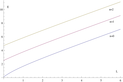
Figure 1: The energy $E$ for $a=1$, $b=\frac{1}{2}$, $d=3$ as a function of $L=\ell$ for $n=0,1,2.$

III The asymptotic iteration method and some related results

The asymptotic iteration method (AIM) was originally introduced aim to investigate the solutions of differential equations of the form

$$y^{\prime\prime}=\lambda_{0}(r)y^{\prime}+s_{0}(r)y,\quad\quad({}^{\prime}={d\over dr})$$ (12)

where $\lambda_{0}(r)$ and $s_{0}(r)$ are $C^{\infty}-$differentiable functions. A key feature of this method is to note the invariant structure of the right-hand side of (12) under further differentiation. Indeed, if we differentiate (12) with respect to $r$, we obtain

$$y^{\prime\prime\prime}=\lambda_{1}y^{\prime}+s_{1}y$$ (13)

where $\lambda_{1}=\lambda_{0}^{\prime}+s_{0}+\lambda_{0}^{2}$ and $s_{1}=s_{0}^{\prime}+s_{0}\lambda_{0}.$ If we find the second derivative of equation (12), we obtain

$$y^{(4)}=\lambda_{2}y^{\prime}+s_{2}y$$ (14)

where $\lambda_{2}=\lambda_{1}^{\prime}+s_{1}+\lambda_{0}\lambda_{1}$ and $s_{2}=s_{1}^{\prime}+s_{0}\lambda_{1}.$ Thus, for $(n+1)^{th}$ and $(n+2)^{th}$ derivative of (12), $n=1,2,\dots$, we have

$$y^{(n+1)}=\lambda_{n-1}y^{\prime}+s_{n-1}y$$ (15)

and

$$y^{(n+2)}=\lambda_{n}y^{\prime}+s_{n}y$$ (16)

respectively, where

$$\lambda_{n}=\lambda_{n-1}^{\prime}+s_{n-1}+\lambda_{0}\lambda_{n-1}\hbox{ ~{}~{}and~{}~{} }s_{n}=s_{n-1}^{\prime}+s_{0}\lambda_{n-1}.$$ (17)

From (15) and (16) we have

$$\lambda_{n}y^{(n+1)}-\lambda_{n-1}y^{(n+2)}=\delta_{n}y{\rm~{}~{}~{}where~{}~{}~{}}\delta_{n}=\lambda_{n}s_{n-1}-\lambda_{n-1}s_{n}.$$ (18)

Clearly, from (18) if $y$, the solution of (12), is a polynomial of degree $n$, then $\delta_{n}\equiv 0$. Further, if $\delta_{n}=0$, then $\delta_{n^{\prime}}=0$ for all $n^{\prime}\geq n$. In an earlier paper aim we proved the principal theorem of AIM, namely

Theorem 1 aim . Given $\lambda_{0}$ and $s_{0}$ in $C^{\infty}(a,b),$ the differential equation (12) has the general solution

$$y(r)=\exp\left(-\int\limits^{r}{s_{n-1}(t)\over\lambda_{n-1}(t)}dt\right)\left[C_{2}+C_{1}\int\limits^{r}\exp\left(\int\limits^{t}(\lambda_{0}(\tau)+2{s_{n-1}\over\lambda_{n-1}}(\tau))d\tau\right)dt\right]$$ (19)

if for some $n>0$

$$\delta_{n}=\lambda_{n}s_{n-1}-\lambda_{n-1}s_{n}=0.$$ (20)

where $\lambda_{n}$ and $s_{n}$ are given by (17). Recently, it has been shown aim1 that the termination condition (20) is necessary and sufficient for the differential equation (12) to have polynomial-type solutions of degrees at most $n$, as we may conclude from Eq.(18). Thus, using Theorem 1, we can now find the necessary and sufficient conditions saad for the polynomial solutions of the differential equation

$$(a_{3,0}r^{3}+a_{3,1}r^{2}+a_{3,2}r+a_{3,3})~{}y^{\prime\prime}+(a_{2,0}r^{2}+a_{2,1}r+a_{2,2})~{}y^{\prime}-(\tau_{1,0}r+\tau_{1,1})~{}y=0,$$ (21)

where $a_{k,j},k=3,2,1,j=0,1,2,3$ are constants. These conditions are reported in the follow theorem. Theorem 2 [saad Theorem 5]. The second-order linear differential equation (21) has a polynomial solution of degree $n$ if

$$\tau_{1,0}=n(n-1)~{}a_{3,0}+n~{}a_{2,0},\quad n=0,1,2,\dots,$$ (22)

provided $a_{3,0}^{2}+a_{2,0}^{2}\neq 0$ along with the vanishing of $(n+1)\times(n+1)$-determinant $\Delta_{n+1}$ given by

$\Delta_{n+1}$  =   $\beta_{0}~{}~{}$ $\alpha_{1}$ $\eta_{1}$ $\gamma_{1}$ $\beta_{1}$ $\alpha_{2}$ $\eta_{2}$ $\gamma_{2}$ $\beta_{2}$ $\alpha_{3}$ $\eta_{3}$ $\ddots$ $\ddots$ $\ddots$ $\ddots$ $\gamma_{n-2}$ $\beta_{n-2}$ $\alpha_{n-1}$ $\eta_{n-1}$ $\gamma_{n-1}$ $\beta_{n-1}$ $\alpha_{n}$ $\gamma_{n}$ $\beta_{n}$   =  0

where all the other entires are zeros and

$$\beta_{n} =\tau_{1,1}-n((n-1)a_{3,1}+a_{2,1})$$

$$\alpha_{n} =-n((n-1)a_{3,2}+a_{2,2})$$

$$\gamma_{n} =\tau_{1,0}-(n-1)((n-2)a_{3,0}+a_{2,0})$$

$$\eta_{n} =-n(n+1)a_{3,3}.$$ (23)

Here $\tau_{1,0}$ is fixed for a given $n$ in the determinant $\Delta_{n+1}=0$ (the degree of the polynomial solution). The coefficients of the polynomial solutions $y_{n}(r)=\sum_{i=0}^{n}c_{i}r^{i}$ satisfies the four-term recursive relation

$$(i+2)(i+1)a_{3,3}c_{i+2}+\left[i(i+1)a_{3,2}+(i+1)a_{2,2}\right]c_{i+1}+\left[i(i-1)a_{3,1}+ia_{2,1}-\tau_{1,1}\right]c_{i}$$

$$+\left[(i-1)(i-2)a_{3,0}+(i-1)a_{2,0}-\tau_{1,0}\right]c_{i-1}=0.$$ (24)

The results of this theorem go beyond the question of finding the polynomial solutions of the second-order linear differential equation

$$(a_{2,0}r^{2}+a_{2,1}r+a_{2,2})~{}y^{\prime\prime}+(a_{1,0}r+a_{1,1})~{}y^{\prime}-\tau_{0,0}~{}y=0.$$ (25)

Indeed Eq.(25) has a nontrivial polynomial solution of degree (exactly) $n\in\mathbb{N}$ (the set of nonnegative integers) if, for fixed $n$,

$$\tau_{0,0}=n(n-1)~{}a_{2,0}+n~{}a_{1,0},\quad n=0,1,2,\dots$$ (26)

provided $a_{2,0}^{2}+a_{1,0}^{2}\neq 0$ where the polynomials $y_{n}$, up to a multiplicative constant, may be readily obtained from the three-term recurrence relation:

$$y_{n+2}=\bigg{[}A_{n}x+B_{n}\bigg{]}y_{n+1}+C_{n}y_{n},\quad n\geq 0$$ (27)

with the coefficients given by

$$A_{n} ={((2n+1)a_{2,0}+a_{1,0})(2(n+1)a_{2,0}+a_{1,0})\over(na_{2,0}+a_{1,0})},$$

$$B_{n} ={((2n+1)a_{2,0}+a_{1,0})(2n(n+1)a_{2,0}a_{2,1}+2(n+1)a_{1,0}a_{2,1}-2a_{1,1}a_{2,0}+a_{1,0}a_{1,1})\over(na_{2,0}+a_{1,0})(2na_{2,0}+a_{1,0})}\bigg{]},$$

$$C_{n} ={(n+1)(2(n+1)a_{2,0}+a_{1,0})((4a_{2,2}a_{2,0}^{2}-a_{2,0}a_{2,1}^{2})n^{2}+(4a_{2,0}a_{1,0}a_{2,2}-a_{1,0}a_{2,1}^{2})n+a_{1,0}^{2}a_{2,2}-a_{1,1}a_{1,0}a_{2,1}+a_{2,0}a_{1,1}^{2})\over(na_{2,0}+a_{1,0})(2na_{2,0}+a_{1,0})},$$

initiated with

$$y_{0}=1,\quad y_{1}=a_{1,0}x+a_{1,1}.$$

In the next sections, we shall apply the result of theorem 2 to study the possible quasi-exact analytic solutions for the $d$-dimension Schrödinger equation (3) for unconstrained and constrained Coulomb plus harmonic oscillator potential (4). We shall also apply AIM, theorem 1, to obtain accurate approximations for arbitrary potential parameters, again, for the unconstrained and constrained $d$-dimensional Schrödinger equation (3).

IV Exact and approximate solutions for unconstrained potential $V(r)$

IV.1 Exact bound-state solutions of a Coulomb plus harmonic oscillator potential in $d$-dimensions

In this section, we consider the $d$-dimensional Schrödinger equation

$$\left[-{1\over 2}\left({d^{2}\over dr^{2}}-{(k-1)(k-3)\over 4r^{2}}\right)-{a\over r}+br^{2}\right]u_{nl}^{d}(r)=E_{nl}^{d}u_{nl}^{d}(r),\quad 0<r<\infty.$$ (28)

In order to solve this equation by using AIM, the first step is to transform (28) into the standard form (12). To this end, we note that the differential equation (28) has one regular singular point at $r=0$ and an irregular singular point at $r=\infty$ and, since for large $r$, the harmonic oscillator term dominates, the asymptotic solution of (28) as $r\rightarrow\infty$ is $u_{r\rightarrow\infty}\sim\exp({-{\sqrt{b/2}~{}r^{2}}})$; meanwhile the indicial equation of (28) at the regular singular point $r=0$ yields

$$s(s-1)-{1\over 4}(k-1)(k-3)=0,$$ (29)

which is solved by

$$s_{1}={1\over 2}(3-k),\quad s_{2}={1\over 2}(k-1).$$

The value of $s$, in Eq.(29), determines the behavior of $u_{nl}^{d}(r)$ for $r\rightarrow 0$, and only $s>1/2$ is acceptable, since only in this case is the mean value of the kinetic energy finite landau . Thus, the exact solution of (28) may assume the form

$$u_{nl}^{d}(r)=r^{{1\over 2}(k-1)}\exp(-\sqrt{b\over 2}~{}r^{2})~{}f_{n}(r),\quad k=d+3l,$$ (30)

where we note that $u_{nl}^{d}(r)\sim r^{{1\over 2}(k-1)}$ as $r\rightarrow 0$. On substituting this ansatz wave function into (28), we obtain the differential equation for $f_{n}(r)$ as

$$rf_{n}^{\prime\prime}(r)+\left(-2r^{2}\sqrt{2b}+k-1\right)f_{n}^{\prime}(r)+\left[\left(2E_{nl}^{d}-k\sqrt{2b}\right)r+2a\right]f_{n}(r)=0.$$ (31)

This equation is a special case of the differential equation (21) with $a_{3,0}=a_{3,1}=a_{3,3}=a_{2,1}=0$, $a_{3,2}=1$, $a_{2,0}=-2r^{2}\sqrt{2b},~{}a_{2,2}=k-1$, $\tau_{1,0}=-2E_{nl}^{d}+k\sqrt{2b}$ and $\tau_{1,1}=-2a$. Thus, the necessary condition for the polynomial solutions of Eq.(31) is

$$E_{nl}^{d}=(2n^{\prime}+k)\sqrt{b\over 2},\quad n^{\prime}=0,1,2,\dots.$$ (32)

and the sufficient condition follows from the vanishing of the tridiagonal determinant $\Delta_{n+1}=0$, $n=0,1,2,\dots$, namely

$\Delta_{n+1}$  =   $\beta_{0}~{}~{}$ $\alpha_{1}$ $\gamma_{1}$ $\beta_{1}$ $\alpha_{2}$ $\gamma_{2}$ $\beta_{2}$ $\alpha_{3}$ $\ddots$ $\ddots$ $\ddots$ $\gamma_{n-2}$ $\beta_{n-2}$ $\alpha_{n-1}$ $\gamma_{n-1}$ $\beta_{n-1}$ $\alpha_{n}$ $\gamma_{n}$ $\beta_{n}$   =  0

where its entries are expressed in terms of the parameters of Eq.(31) by

$$\beta_{n} =-2a,\quad\alpha_{n}=-n(n+k-2),\quad\gamma_{n}=-2(n^{\prime}-n+1)\sqrt{2b},$$ (33)

where $n^{\prime}=n$ is fixed by the size of the determinant $\Delta_{n+1}=0$ and represent the degree of the polynomial solution of Eq.(31). We may note that, since the off-diagonal entries $\alpha_{i}$ and $\gamma_{i}$ of the tridiagonal determinant satisfy the identity

$$\alpha_{i}\gamma_{i}>0,\quad\forall~{}~{}i=1,2,\dots,$$

the latent roots of the determinant $\Delta_{n+1}$ are all real and distinct arscott . Further, we can easily show that the determinant (33) satisfies a three-term recurrence relation

$$\Delta_{i}=\beta_{i-1}\Delta_{i-1}-\gamma_{i-1}\alpha_{i-1}\Delta_{i-2},\quad\Delta_{0}=1,~{}~{}\Delta_{-1}=0,\quad i=1,2,\dots$$ (34)

which can be used to compute the determinant $\Delta_{i}$ (and thus the sufficient conditions), recursively in terms of lower order determinants. In this case, however, we must fix $n^{\prime}$ for each of the sub-determinants used in computing (34). For example, in the case of $n^{\prime}=n=1$ (corresponding to a polynomial solution of degree one), we have

$\Delta_{2}$  =   $-2a$ $-(k-1)$ $-2\sqrt{2b}$ $-2a$   = $\beta_{1}\Delta_{1}-\gamma_{1}\alpha_{1}\Delta_{0}$=$(-2a)(-2a)-(-2\sqrt{2b})(-(k-1))(1)$=$4a^{2}-2\sqrt{2b}(k-1),$

that is, the condition of the potential parameters reads

$$2a^{2}-\sqrt{2b}(k-1)=0.$$ (35)

For $n^{\prime}=n=2$ (corresponding to a second-degree polynomial solution)

$\Delta_{3}$  =   $-2a~{}~{}$ $-(k-1)$ $0$ $-4\sqrt{2b}$ $-2a$ $-2k$ 0 $-2\sqrt{2b}$ $-2a$  =$\beta_{2}\Delta_{2}-\gamma_{2}\alpha_{2}\Delta_{1}$=$(-2a)\begin{tabular}[]{|ll|}$-2a~{}~{}$&$-(k-1)$\\ $-4\sqrt{2b}$&$-2a$\end{tabular}-(-2\sqrt{2b})(-2k)(-2a)$

= $(-2a)[(-2a)\Delta_{1}-(-4\sqrt{2b})(-(k-1))\Delta_{0}$]+$8ka\sqrt{2b}$ = $8a(-a^{2}+2\sqrt{2b}k-\sqrt{2b})$

Consequently, we must have

$$a(a^{2}-2\sqrt{2b}k+\sqrt{2b})=0.$$ (36)

In Table I, we give the conditions on the potential parameters to allow for polynomial solutions, from theorem 2.

Table 1: Conditions on the parameters $a$ and $b$ for the exact solutions of Eq.(28) with $E_{nl}^{d}=(2n+k)\sqrt{b/2}$, $k=d+2l$.

$n$	$\Delta_{n+1}=0$
0	$a=0$
1	$2a^{2}-(k-1)\sqrt{2b}=0$
2	$a(a^{2}-(2k-1)\sqrt{2b})=0$
3	$4a^{4}-20a^{2}\sqrt{2b}k-18b(1-k^{2})=0$
4	$a(a^{4}-5\sqrt{2b}(2k+1)a^{2}+4b(8k^{2}+8k-7))=0$
5	$8a^{6}-140\sqrt{2b}(k+1)a^{4}+4b(-65+518k+259k^{2})a^{2}-450b\sqrt{2b}(k-1)(k+3)(k+1)=0$

It must be clear that although $n$, the degree of the polynomial solution, it is not necessarily an indication as to the number of the zeros of the wave function (node number): further analysis of the roots of $f_{n}(r)$ is usually needed to compute the zeros of the wavefunction. The polynomial solutions $f_{n^{\prime}}(r)=\sum_{i=0}^{n^{\prime}}c_{i}r^{i}$ can be easily constructed for each $n^{\prime}$ since, in this case, the coefficients $c_{i}$ satisfy the three-term recurrence relation (see Eq.(III))

$$c_{-1}=0,\quad c_{0}=1,\quad c_{i+1}=-{2ac_{i}+2(n^{\prime}-i+1)\sqrt{2b}c_{i-1}\over(i+1)(i+k-1)},~{}~{}i=0,1,\dots,n^{\prime}-1,$$ (37)

where $n^{\prime}$ is the degree of the polynomial solution. When $n^{\prime}=0$, $f_{0}(r)=1$. For the first-degree polynomial solution, $n^{\prime}=1,i=0$, we have

$$c_{1}=-{2a\over k-1},$$

that is

$$f_{1}(r)=1-{2a\over k-1}r,\quad\mbox{where}\quad 2a^{2}-(k-1)\sqrt{2b}=0.$$ (38)

We may further note for $a<0$, there is no root of $f_{1}(r)=0$ and the un-normalized wave function reads

$$u_{0l}^{d}(r)=r^{{1\over 2}(d+2l-1)}\exp\left(-{a^{2}r^{2}\over d+2l-1}\right)~{}\left(1-{2ar\over d+2l-1}\right),\quad a<0$$ (39)

which represents a ground-state wave function in every subspace labeled by $d$ and $l$. For $a>0$, there is only one root of $f_{1}$ and the wave function

$$u_{1l}^{d}(r)=r^{{1\over 2}(d+2l-1)}\exp\left(-{a^{2}r^{2}\over d+2l-1}\right)~{}\left(1-{2ar\over d+2l-1}\right),\quad a>0$$ (40)

which represents a first excited-state in each subspace labeled by $d$ and $l$. The zero of this wave function is located at

$$R={k-1\over 2a},\quad k=d+2l,\quad a>0.$$ (41)

In both cases, $a>0$ or $a<0$, the exact eigenvalues are given by

$$E_{0l}^{d}\equiv E_{1l}^{d}\equiv E_{1l\pm 1}^{d\mp 2}={a^{2}(d+2l+2)\over(2d+4l-1)},\quad\quad\lim_{d\rightarrow\infty}E_{1l\pm 1}^{d\mp 2}={a^{2}\over 2}.$$ (42)

For second-degree polynomial solution, $n^{\prime}=2,i=0,1$, we have for the polynomial solution, $f_{2}(r)=c_{0}+c_{1}r+c_{2}r^{2}$, coefficients

$$c_{0}=1,\quad c_{1} =-{2a\over k-1}\quad\mbox{and}\quad c_{2}={2(a^{2}-\sqrt{2b}(k-1))\over k(k-1)}$$

and the polynomial solution then reads

$$f_{2}(r)=1-{2ar\over(k-1)}+{2a^{2}r^{2}\over(k-1)(2k-1)},$$ (43)

where $a(a^{2}-(2k-1)\sqrt{2b})=0$ from which we may conclude that $a^{2}-\sqrt{2b}(k-1)>0$. Therefore, the wave function $f_{2}(r)$ has either two roots or no root based on the value of $a>0$ or $a<0$, respectively. For $a>0$, we have a second-excited state wave function

$$u_{2l}^{d}(r)=r^{{1\over 2}(d+2l-1)}\exp\left(-{a^{2}r^{2}\over 2(2d+4l-1)}\right)~{}\left(1-{2ar\over d+2l-1}+{2a^{2}r^{2}\over(d+2l-1)(2d+4l-1)}\right),\quad a>0,$$ (44)

which has two zeros at

$$R_{1}={2k-1+\sqrt{2k-1}\over 2a},\quad R_{2}={2k-1-\sqrt{2k-1}\over 2a},\quad k=d+2l,\quad a>0.$$ (45)

For $a<0$, we have a ground-state wave function

$$u_{2l}^{d}(r)=r^{{1\over 2}(d+2l-1)}\exp\left(-{a^{2}~{}r^{2}\over 2(2d+4l-1)}\right)~{}\left(1-{2ar\over d+2l-1}+{2a^{2}r^{2}\over(d+2l-1)(2d+4l-1)}\right),\quad a<0.$$ (46)

In either case, $a>0$ or $a<0$, the exact eigenvalues reads

$$E_{0l}^{d}\equiv E_{2l}^{d}\equiv E_{2l\pm 1}^{d\mp 2}={a^{2}(d+2l+4)\over 2(2d+4l-1)},\quad\quad\lim_{d\rightarrow\infty}E_{2l\pm 1}^{d\mp 2}={a^{2}\over 4}.$$ (47)

For third-degree polynomial solution, $n^{\prime}=3,i=0,1,2$, we have for the polynomial coefficients $f_{3}(r)=c_{0}+c_{1}r+c_{2}r^{2}+c_{3}r^{3}$ that

$$c_{0}=1,\quad c_{1} =-{2a\over k-1},\quad c_{2}={(2a^{2}-3\sqrt{2b}(k-1))\over k(k-1)},\quad c_{3}=-{2a(2a^{2}-7\sqrt{2b}k+3\sqrt{2b})\over 3(k-1)k(k+1)},$$

and the polynomial solution then reads

$$f_{3}(r)=1-{2a\over k-1}r+{(2a^{2}-3(k-1)\sqrt{2b})\over k(k-1)}r^{2}-{2a(2a^{2}-(7k-3)\sqrt{2b})\over 3(k-1)k(k+1)}r^{3},$$ (48)

where the potential parameters satisfy the condition $4a^{4}-20a^{2}\sqrt{2b}k+18b(k^{2}-1)=0$ which may be solved in terms of $\sqrt{2b}$ as

$$\sqrt{2b}={2a^{2}(5k\pm\sqrt{16k^{2}+9})\over 9(k^{2}-1)}.$$ (49)

From this we have

$$f_{3}^{+}(r)=1-{2ar\over k-1}-{2a^{2}\over 3}{(2k-3+\sqrt{16k^{2}+9})r^{2}\over(k+1)k(k-1)}+{4\over 9}{a^{3}(26k^{2}-15k+9+(7k-3)\sqrt{16k^{2}+9})r^{3}\over 3(k-1)^{2}k(k+1)^{2}},$$ (50)

and

$$f_{3}^{-}(r)=1-{2ar\over k-1}-{2a^{2}\over 3}{(2k-3-\sqrt{16k^{2}+9})r^{2}\over(k+1)k(k-1)}+{4\over 9}{a^{3}(26k^{2}-15k+9-(7k-3)\sqrt{16k^{2}+9})r^{3}\over 3(k-1)^{2}k(k+1)^{2}}.$$ (51)

The polynomial $f_{3}^{+}(r)$ has two roots if $a>0$ and only one root if $a<0$ for all $r>0$; while $f_{3}^{-}(r)$ has no root for $a<0$ and has three roots for $a>0$ (the results that follow from Descartes’ rule of signs). In each of these cases, the eigenvalues are given by

$$E_{3l}^{d\pm}={a^{2}\over 9}{(d+2l+6)\left(5d+10l\pm\sqrt{16(d+2l)^{2}+9}\right)\over(d+2l-1)(d+2l+1)},\quad a\neq 0.$$ (52)

We can also show for the fourth-degree polynomial solution, $n^{\prime}=4,i=0,1,2,3$, we have

$$f_{4}(r)=1-{2a\over k-1}r+{(2a^{2}-4\sqrt{2b}(k-1))\over k(k-1)}r^{2}+{4a[-a^{2}+5\sqrt{2b}k-2\sqrt{2b}]\over 3(k-1)k(k+1)}r^{3}+{2[a^{4}-(1+8k)\sqrt{2b}a^{2}+12b(k^{2}-1)]\over 3(k+2)(k+1)k(k-1)}r^{4}$$ (53)

subject to $a(a^{4}-5\sqrt{2b}(2k+1)a^{2}+4b(8k^{2}+8k-7))=0$ and in this case

$$E_{4l}^{d\pm}={a^{2}\over 8}{(k+8)\left(10k+5\pm 3\sqrt{(2k+1)^{2}+8}\right)\over 2(2k+1)^{2}-9},\quad k=d+2l,a\neq 0$$ (54)

and similarly for other cases. Indeed, using the recurrence relation, Eq.(37), it is straightforward to compute explicitly the polynomial solution of any required degree.

IV.2 Approximate solutions for arbitrary potential parameters on half-line

For arbitrary values of the potential parameters $a$ and $b$ that do not necessarily obey the above conditions, we may use AIM directly to compute the eigenvalues accurately, as the zeros of the termination condition (20). The method can be used, as well, to test the exact solutions we obtained in the above section. To utilize AIM, we start with

$$\left\{\begin{array}[]{l}\lambda_{0}(r)=2\sqrt{2b}~{}r-{(k-1)\over r},\\ \\ s_{0}(r)=-{(2E_{nl}^{d}-k\sqrt{2b})}-{2a\over r}\end{array}\right.$$ (55)

and computing the AIM sequences $\lambda_{n}$ and $s_{n}$ as given by Eq.(17). We should note that for given values of the potential parameters $a$, $b,$ and of $k=d+2l$, the termination condition $\delta_{n}=\lambda_{n}s_{n-1}-\lambda_{n-1}s_{n}=0$ yields an expression that depends on both $r$ and $E$. In order to use AIM as an approximation technique for computing the eigenvalues $E$ we need to feed AIM with an initial value of $r=r_{0}$ that could stabilize AIM (that is, to avoid oscillations). For our calculations, we have found that $r_{0}=3$ stablizes AIM and allows us to compute the eigenvalues for arbitrary $k=d+2l$ and $n$ as shown in Table 2. There is no magical assertion about $r_{0}=3$, indeed using an exact solvable case, say $E=2.5$ with $d=3,l=0,n^{\prime}=1$ for $a=1$ and $b=1/2$, we may approximate $r=r_{0}$ by means of $E-V(r)=0$ which yields $r_{0}\sim 2.4$ as an initial starting value for the AIM process. The eigenvalue computations in Table 2 were done using Maple version 13 running on an IBM architecture personal computer, where we used a high-precision environment. In order to accelerate our computation we have written our own code for a root-finding algorithm instead of using the default procedure Solve of Maple 13.

Table 2: Eigenvalues $E_{n0}^{d=2,3,4,5,6,7}$ for $V(r)=-1/r+r^{2}/2$. The initial value utilize AIM is $r_{0}=3$. The subscript $N$ refer to the number of iteration used by AIM.

$n$	$E_{n0}^{d=2}$	$n$	$E_{n0}^{d=3}$
0	$-1.836~{}207~{}439~{}051~{}476~{}488_{N=78}$	0	$~{}0.179~{}668~{}484~{}653~{}553~{}873_{N=71}$
1	$~{}~{}1.576~{}895~{}542~{}024~{}474~{}773_{N=71}$	1	$~{}2.500~{}000~{}000~{}000~{}000~{}000_{N=3~{}Exact}$
2	$~{}~{}3.828~{}388~{}290~{}161~{}145~{}035_{N=64}$	2	$~{}4.631~{}952~{}408~{}873~{}053~{}214_{N=59}$
3	$~{}~{}5.963~{}137~{}645~{}125~{}787~{}098_{N=60}$	3	$~{}6.712~{}595~{}725~{}661~{}429~{}760_{N=58}$
4	$~{}~{}8.052~{}626~{}115~{}348~{}259~{}660_{N=59}$	4	$~{}8.769~{}519~{}600~{}328~{}899~{}714_{N=57}$
5	$~{}10.118~{}396~{}975~{}257~{}306~{}974_{N=58}$	5	$10.812~{}924~{}292~{}726~{}383~{}736_{N=56}$
6	$~{}12.169~{}728~{}962~{}611~{}565~{}630_{N=58}$	6	$12.847~{}666~{}480~{}105~{}796~{}414_{N=55}$
$n$	$E_{n0}^{d=4}\equiv E_{n1}^{2}$	$n$	$E_{n0}^{d=5}\equiv E_{n1}^{3}$
0	$~{}1.039~{}629~{}453~{}693~{}666~{}062_{N=63}$	0	$~{}1.709~{}018~{}091~{}123~{}552~{}219_{N=60}$
1	$~{}3.191~{}127~{}807~{}756~{}594~{}984_{N=58}$	1	$~{}3.801~{}929~{}609~{}626~{}278~{}046_{N=55}$
2	$~{}5.273~{}870~{}062~{}099~{}308~{}315_{N=57}$	2	$~{}5.860~{}357~{}172~{}819~{}176~{}603_{N=55}$
3	$~{}7.329~{}588~{}502~{}119~{}331~{}779_{N=54}$	3	$~{}7.902~{}317~{}748~{}608~{}790~{}676_{N=52}$
4	$~{}9.371~{}002~{}235~{}676~{}830~{}145_{N=53}$	4	$~{}9.934~{}707~{}216~{}855~{}127~{}521_{N=51}$
5	$11.403~{}631~{}794~{}919~{}620~{}038_{N=53}$	5	$11.960~{}878~{}210~{}587~{}747~{}585_{N=51}$
6	$13.430~{}355~{}223~{}285~{}870~{}950_{N=53}$	6	$13.982~{}705~{}338~{}927~{}982~{}296_{N=50}$
$n$	$E_{n0}^{d=6}\equiv E_{n1}^{4}\equiv E_{n2}^{2}$	$n$	$E_{n0}^{d=7}\equiv E_{n1}^{5}\equiv E_{n2}^{3}$
0	$~{}2.311~{}633~{}609~{}259~{}797~{}633_{N=56}$	0	$~{}2.882~{}228~{}025~{}698~{}769~{}118_{N=52}$
1	$~{}4.376~{}287~{}059~{}247~{}773~{}643_{N=52}$	1	$~{}4.930~{}673~{}420~{}047~{}524~{}772_{N=50}$
2	$~{}6.420~{}575~{}455~{}465~{}976~{}803_{N=52}$	2	$~{}6.965~{}837~{}318~{}124~{}071~{}248_{N=48}$
3	$~{}8.453~{}864~{}208~{}404~{}376~{}310_{N=49}$	3	$~{}8.993~{}183~{}541~{}000~{}280~{}301_{N=47}$
4	$~{}10.480~{}309~{}010~{}248~{}775~{}417_{N=50}$	4	$~{}11.015~{}405~{}735~{}685~{}306~{}483_{N=47}$
5	$12.502~{}107~{}717~{}572~{}917~{}269_{N=48}$	5	$13.034~{}024~{}645~{}001~{}717~{}876_{N=47}$
6	$14.520~{}559~{}118~{}487~{}876~{}168_{N=48}$	6	$15.049~{}980~{}236~{}362~{}344~{}263_{N=47}$

V Exact and approximate solutions for constrained potential

V.1 Analytic solutions

We now consider the $d$-dimensional Schrödinger equation

$$\left[-{1\over 2}\left({d^{2}\over dr^{2}}-{(k-1)(k-3)\over 4r^{2}}\right)+V(r)\right]u_{nl}^{d}(r)=E_{nl}^{d}u_{nl}^{d}(r),\quad 0<r<R,$$ (56)

where

$$V(r)=\left\{\begin{array}[]{ll}-{a\over r}+br^{2},&\mbox{ if $0<r<R$}\\ \\ \infty&\mbox{ if $r\geq R$}\end{array}\right.$$ (57)

and $u_{nl}^{d}(0)=u_{nl}^{d}(R)=0$. We may assume the following ansatz for the wave function

$$u_{nl}^{d}(r)=r^{{1\over 2}(k-1)}(R-r)\exp\left(-\sqrt{b\over 2}~{}r^{2}\right)~{}f_{n}(r),\quad k=d+2l.$$ (58)

where $R$ is the radius of confinement, and the $(R-r)$ factor ensures that the radial wavefunction $u_{nl}^{d}(r)$ vanishes at the boundary $r=R$. On substituting (49) into (47), we obtain the following second-order differential equation for the functions $f_{n}(r)$:

$$f_{n}^{\prime\prime}(r) =-2\left({k-1\over 2r}-{1\over R-r}-\sqrt{2b}~{}r\right)f_{n}^{\prime}(r)$$

$$-{1\over r(R-r)}\bigg{[}(-2E_{nl}^{d}+(k+2)\sqrt{2b})r^{2}+(R(2E_{nl}^{d}-k\sqrt{2b})-2a)r-k+1+2Ra\bigg{]}f_{n}(r).$$ (59)

We note that this equation reduces to Eq.(31) as $R\rightarrow\infty$. Equation (V.1) can be written as

$$[-r^{2}+Rr]f_{n}^{\prime\prime}(r) +[2\sqrt{2b}r^{3}-2\sqrt{2b}Rr^{2}-(k+1)r+(k-1)R]f_{n}^{\prime}(r)$$

$$+{\bigg{[}(-2E_{nl}^{d}+(k+2)\sqrt{2b})r^{2}+(R(2E_{nl}^{d}-k\sqrt{2b})-2a)r+2Ra-k+1\bigg{]}}f_{n}(r)=0$$ (60)

This differential equation cannot be studied using Theorem 2. Consequently a further investigation of the following class of differential equations

$$(a_{4,0}r^{4}+a_{4,1}r^{3}+a_{4,2}r^{2} +a_{4,3}r+a_{4,4})y^{\prime\prime}+(a_{3,0}r^{3}+a_{3,1}r^{2}+a_{3,2}r+a_{3,3})y^{\prime}-(\tau_{2,0}r^{2}+\tau_{2,1}r+\tau_{2,2})y=0,$$ (61)

is needed. Indeed, by using Theorem 1 and a proof along the lines of the proof of Theorem 2, we are able to establish the following: Theorem 3. The second-order linear differential equation (61) has a polynomial solution $y(r)=\sum_{k=0}^{n}c_{k}r^{k}$ if

$$\tau_{2,0}=n(n-1)~{}a_{4,0}+n~{}a_{3,0},\quad n=0,1,2,\dots,$$ (62)

provided $a_{4,0}^{2}+a_{3,0}^{2}\neq 0$ where the polynomial coefficients $c_{n}$ satisfy the five-term recurrence relation

$$((n-2) (n-3)a_{4,0}+(n-2)a_{3,0}-\tau_{2,0})c_{n-2}+((n-1)(n-2)a_{4,1}+(n-1)a_{3,1}-\tau_{2,1})c_{n-1}$$

$$+(n(n-1)a_{4,2}+na_{3,2}-\tau_{2,2})c_{n}+(n(n+1)a_{4,3}+(n+1)a_{3,3})c_{n+1}+(n+2)(n+1)a_{4,4}c_{n+2}=0$$ (63)

with $c_{-2}=c_{-1}=0$. In particular, for the zero-degree polynomials $c_{0}\neq 0$ and $c_{n}=0,~{}n\geq 1$, we have

$$\tau_{2,2}=0,~{}\tau_{2,1}=0,~{}\tau_{2,0}=0.$$ (64)

For the first-degree polynomial solution, $c_{0}\neq 0,\quad c_{1}\neq 0$ and $c_{n}=0,n\geq 2$, we must have

$$\tau_{2,0}=a_{3,0}$$ (65)

along with the vanishing of the two $2\times 2$-determinants, simultaneously,

$$\left|\begin{array}[]{ccc}-\tau_{2,2}&a_{3,3}\\ -\tau_{2,1}&a_{3,2}-\tau_{2,2}\end{array}\right|=0,\quad\mbox{and}\quad\left|\begin{array}[]{ccc}-\tau_{2,2}&a_{3,3}\\ -a_{3,0}&a_{3,1}-\tau_{2,1}\end{array}\right|=0.$$ (66)

For the second-degree polynomial solution, $c_{0}\neq 0,c_{1}\neq 0,c_{2}\neq 0$ and $c_{n}=0$ for $n\geq 3$, we must have

$$\tau_{2,0}=2~{}a_{4,0}+2a_{3,0}$$ (67)

along with the vanishing of the two $3\times 3$-determinants, simultaneously,

$$\left|\begin{array}[]{ccc}-\tau_{2,2}&a_{3,3}&2a_{4,4}\\ -\tau_{2,1}&a_{3,2}-\tau_{2,2}&2a_{4,3}+2a_{3,3}\\ -2a_{4,0}-2a_{3,0}&a_{3,1}-\tau_{2,1}&2a_{4,2}+2a_{3,2}-\tau_{2,2}\end{array}\right|=0,~{}\mbox{and}~{}\left|\begin{array}[]{ccc}-\tau_{2,2}&a_{3,3}&2a_{4,4}\\ -\tau_{2,1}&a_{3,2}-\tau_{2,2}&2a_{4,3}+2a_{3,3}\\ 0&-2a_{4,0}-a_{3,0}&2a_{4,1}+2a_{3,1}-\tau_{2,1}\end{array}\right|=0,$$ (68)

and so on, for higher-order polynomial solutions. The vanishing of these determinants can be regarded as the conditions under which the coefficients $\tau_{2,1}$ and $\tau_{2,2}$ of Eq.(61) are determined. Using Theorem 3, we may note, with $a_{4,0}=a_{4,1}=a_{4,4}=0,a_{4,2}=-1,a_{4,3}=R,a_{3,0}=2\sqrt{2b},a_{3,1}=-2\sqrt{2b}R,a_{3,2}=-(k+1),a_{3,3}=(k-1)R,\tau_{2,0}=2E_{nl}^{d}-(k+2)\sqrt{2b},\tau_{2,1}=-(R(2E_{nl}^{d}-k\sqrt{2b})-2a),\tau_{2,2}=-2Ra+k-1$, that the necessary condition for polynomial solutions $f_{n}(r)=\sum_{k=0}^{n}c_{k}r^{k}$ of Eq.(V.1) is

$$E_{nl}^{d}={1\over 2}(2n+k+2)\sqrt{2b},\quad k=d+2l,$$ (69)

where $n$ refers to the degree of the polynomial solution and not necessarily to the number of zeros for the exact wave function. For sufficient conditions, we have for the zero-degree polynomial solution $n=0$, that Eq.(64) yields

$$f_{0}(r)=1,\quad E_{0l}^{d}={1\over 2}(k+2)\sqrt{2b},\quad\mbox{ if}\quad a=R\sqrt{2b}\quad\mbox{and}\quad Ra={1\over 2}(k-1),$$ (70)

where, again, $k=d+2l$. For example, if $a=3,~{}b=4.5$, we have $R=1$ and for $k=d+2l=7$, we have the exact solution

$$E_{00}^{7}=E_{01}^{5}=E_{02}^{3}=13.5$$

and for $a=4,b=8$, we have $R=1$ and for $k=d+2l=9$, we have the exact solution

$$E_{00}^{9}=E_{01}^{7}=E_{02}^{5}=E_{03}^{3}=22.$$

Thus, for the values of the potential parameters $a,b$ and $R$ as given by

$$(a,b,R)=\left({1\over 2R}(2l+d-1),{1\over 8R^{4}}(2l+d-1)^{2},R\right),$$ (71)

we have the exact solutions

$$\left\{\begin{array}[]{l}E_{0l}^{d}={1\over 4R^{2}}(d+2l-1)(d+2l+2),\\ \\ u_{0l}^{d}(r)=r^{{1\over 2}(2l+d-1)}(R-r)\exp(-{d+2l-1\over 4R^{2}}~{}r^{2}).\end{array}\right.$$ (72)

We may note that the confinement size $R=(k-1)/(2a)$ represent the root of the unconfined wave function, (40), with the same energy (compare (42 with (70)).

For first-degree polynomial solution $n=1$, we have using (69), or $\tau_{2,0}=4\sqrt{2b}$,

$$E_{1l}^{d}={1\over 2}(k+4)\sqrt{2b},$$ (73)

along with the two conditions, obtained using (66), which relate the potential parameters by

$$\left\{\begin{array}[]{l}2kRa-k(k-1)-2R^{2}a^{2}+2R^{2}\sqrt{2b}(k-1)=0,\\ \\ 2\sqrt{2b}R^{2}-2Ra+k-1=0.\end{array}\right.$$ (74)

where, in this case, the polynomial solution reads

$$f_{1}(r)=1-{(2Ra+1-k)\over R(k-1)}r.$$ (75)

Thus, for the relations

$$(a,b,R)=\left({2k-1+\sqrt{2k-1}\over 2R},{(k+\sqrt{2k-1})^{2}\over 8R^{4}},R\right),\quad k=d+2l$$ (76)

we have the exact solutions

$$\left\{\begin{array}[]{l}E_{1l}^{d}={1\over 4R^{2}}(k+4)(k+\sqrt{2k-1}),\\ \\ u_{1l}^{d}(r)=r^{{1\over 2}(k-1)}(R-r)\exp(-{k+\sqrt{2k-1}\over 4R^{2}}~{}r^{2})\left(1-{(k+\sqrt{2k-1})\over R(k-1)}r\right).\end{array}\right.$$ (77)

and for

$$(a,b,R)=\left({2k-1-\sqrt{2k-1}\over 2R},{(k-\sqrt{2k-1})^{2}\over 8R^{4}},R\right),\quad k=d+2l,$$ (78)

we have the exact solutions

$$\left\{\begin{array}[]{l}E_{1l}^{d}={1\over 4R^{2}}(k+4)(k-\sqrt{2k-1}),\\ \\ u_{1l}^{d}(r)=r^{{1\over 2}(k-1)}(R-r)\exp(-{k-\sqrt{2k-1}\over 4R^{2}}~{}r^{2})\left(1-{(k-\sqrt{2k-1})\over R(k-1)}r\right).\end{array}\right.$$ (79)

We note that these exact-solutions cases (76) and (78) represent the nodes of the wavefunction in the infinite case (44).

For second-degree polynomial solutions $n=2$, we have the exact eigenvalues

$$E_{nl}^{d}={1\over 2}(k+6)\sqrt{2b}$$ (80)

where $k=d+2l$ and the potential parameters $a$, $b$ and $R$ are related by the following two conditions (obtained from the two determinants in (68)

$$4R^{3}a^{3}-6(k+1)R^{2}a^{2}-2R(R^{2}\sqrt{2b}(7k-3)-3k(k+1))a+3(k-1)(k+1)(3\sqrt{2b}R^{2}-k)=0,$$ (81)

and

$$2R^{2}a^{3}-2R(R^{2}\sqrt{2b}+k)a^{2}-(k-1)(3\sqrt{2b}R^{2}-k)a+6b(k-1)R^{3}=0.$$ (82)

In this case the exact solution reads

$$u_{2l}^{d}=r^{{1\over 2}(k-1)}(R-r)\exp\left(-\sqrt{b\over 2}r^{2}\right)\left(1-{2Ra-k+1\over R(k-1)}r+{(2R^{2}a^{2}-2Rak+k(k-1)-3\sqrt{2b}R^{2}(k-1))\over R^{2}k(k-1)}r^{2}\right).$$ (83)

Again in this case we can show that these exact solutions correspond to the zeros of the wavefunction in the infinite case (50) and (51).

Similar results can be obtained for higher $n$ (the degree of the polynomial solutions). It is important to note that the conditions reported here are for the mixed potential $V(r)=-a/r+br^{2}$, where $a\neq 0$ and $b\neq 0$ (that is to say, neither coefficient is zero).

V.2 Approximate solutions for confined potential with arbitrary parameters

For the arbitrary values of $a,b$ and $R$, not necessarily satisfying the above conditions, we may use AIM directly to compute the eigenvalues with a very high degree of accuracy. This also allows us to verify the exact solutions we obtained in the perevious sections. Similarly to the unconfined case, we start the iteration of the AIM sequence $\lambda_{n}$ and $s_{n}$ with

$$\left\{\begin{array}[]{l}\lambda_{0}(r)=-2\left({k-1\over 2r}-{1\over R-r}-\sqrt{2b}~{}r\right),\\ \\ s_{0}(r)=-{(-2E_{nl}^{d}+(k+2)\sqrt{2b})r^{2}+(R(2E_{nl}^{d}-k\sqrt{2b})-2a)r+2Ra-k+1\over r(R-r)}.\end{array}\right.$$ (84)

where $0<r<R$. It is interesting to note in this case, that, unlike the unconfined case, the roots of the termination condition $\delta_{n}=\lambda_{n}s_{n-1}-\lambda_{n-1}s_{n}=0$ are much easier to handle in the present case. This is due to the fact that $r_{0}$ is now bound within $(0,R)$ for every given $R$. Thus, it is sufficient to start our iteration process with initial value $r_{0}=R/2$. In table 3, we reported the eigenvalues we have computed using AIM for a fixed radius of confinement $R=1$, with $r_{0}=0.5$ as an initial value to seed the AIM process. In general, the computation of the eigenvalues is fast, as is illustrated by the small number of iteration $N$ in Tables 3. The same procedure can be applied to compute the eigenvalues for other values of $a$, $b$ $R$, and arbitrary dimension $d$. The results of AIM may be obtained to any degree of precision, although we have reported our results for only the first eighteen decimal places. It is clear from the table that our results confirm the invariance of the eigenvalues under the transformation $(d,l)\rightarrow(d\mp 2,l\pm 1).$

Table 3: Eigenvalues $E_{nl}^{d=2,4}(a,b;R)$ for $V(r)=-a/r+br^{2},r\in(0,R)$, where $a=\pm 1$, $b=0.5$, $R=1$ and different $n$ and $l$. The subscript $N$ refers to the number of iteration used by AIM.

$n$	$l$	$E_{nl}^{d=2}(1,1/2;1)$	$n$	$l$	$E_{nl}^{d=2}(1,1/2;1)$
0	0	$-1.275~{}615~{}599~{}206~{}285~{}795_{N=32}$	0	0	$~{}-1.275~{}615~{}599~{}206~{}285~{}795_{N=32}$
	1	$~{}~{}5.400~{}467~{}192~{}272~{}980~{}536_{N=26}$	1		$~{}~{}10.924~{}630~{}155~{}130~{}440~{}587_{N=27}$
	2	$~{}11.652~{}661~{}600~{}597~{}110~{}050_{N=24}$	2		$~{}~{}32.734~{}045~{}433~{}763~{}800~{}052_{N=32}$
	3	$~{}19.010~{}259~{}174~{}813~{}201~{}428_{N=24}$	3		$~{}~{}64.522~{}506~{}980~{}951~{}712~{}401_{N=40}$
	4	$~{}27.565~{}689~{}679~{}299~{}850~{}255_{N=25}$	4		$~{}106.243~{}804~{}852~{}673~{}032~{}613_{N=47}$
	5	$~{}37.324~{}795~{}658~{}776~{}520~{}956_{N=28}$	5		$~{}157.875~{}359~{}994~{}443~{}580~{}341_{N=53}$
$n$	$l$	$E_{nl}^{d=2}(-1,1/2;1)$	$n$	$l$	$E_{nl}^{d=2}(-1,1/2;1)$
0	0	$~{}~{}6.107~{}045~{}323~{}129~{}696~{}121_{N=27}$	0	0	$~{}~{}6.107~{}045~{}323~{}129~{}696~{}121_{N=27}$
	1	$~{}~{}9.530~{}081~{}242~{}027~{}809~{}913_{N=24}$	1		$~{}19.534~{}700~{}629~{}074~{}427~{}546_{N=27}$
	2	$~{}15.106~{}527~{}319~{}660~{}138~{}719_{N=24}$	2		$~{}42.295~{}175~{}016~{}376~{}479~{}090_{N=35}$
	3	$~{}22.149~{}694~{}772~{}638~{}116~{}456_{N=24}$	3		$~{}74.728~{}314~{}736~{}027~{}030~{}722_{N=43}$
	4	$~{}30.518~{}339~{}762~{}183~{}359~{}381_{N=27}$	4		$~{}116.935~{}489~{}978~{}445~{}435~{}860_{N=47}$
	5	$~{}40.151~{}787~{}835~{}702~{}316~{}786_{N=29}$	5		$~{}168.956~{}853~{}183~{}684~{}793~{}313_{N=55}$
$n$	$l$	$E_{nl}^{d=4}(1,1/2;1)$	$n$	$l$	$E_{nl}^{d=4}(1,1/2;1)$
0	0	$~{}~{}5.400~{}467~{}192~{}272~{}980~{}536_{N=26}$	0	0	$~{}~{}~{}5.400~{}467~{}192~{}272~{}980~{}536_{N=24}$
	1	$~{}11.652~{}661~{}600~{}597~{}110~{}050_{N=24}$	1		$~{}~{}22.123~{}225~{}647~{}087~{}677~{}088_{N=25}$
	2	$~{}19.010~{}259~{}174~{}813~{}201~{}428_{N=24}$	2		$~{}~{}48.910~{}542~{}938~{}654~{}909~{}374_{N=35}$
	3	$~{}27.565~{}689~{}679~{}299~{}850~{}255_{N=25}$	3		$~{}~{}85.660~{}358~{}190~{}161~{}408~{}159_{N=43}$
	4	$~{}37.324~{}795~{}658~{}776~{}520~{}956_{N=28}$	4		$~{}132.333~{}925~{}295~{}766~{}891~{}686_{N=48}$
	5	$~{}48.278~{}874~{}241~{}139~{}597~{}779_{N=31}$	5		$~{}188.912~{}601~{}544~{}108~{}537~{}448_{N=54}$
$n$	$l$	$E_{nl}^{d=4}(-1,1/2;1)$	$n$	$l$	$E_{nl}^{d=4}(-1,1/2;1)$
0	0	$~{}~{}9.530~{}081~{}242~{}027~{}809~{}913_{N=24}$	0	0	$~{}~{}~{}9.530~{}081~{}242~{}027~{}809~{}913_{N=24}$
	1	$~{}15.106~{}527~{}319~{}660~{}138~{}719_{N=24}$	1		$~{}~{}27.374~{}386~{}080~{}371~{}192~{}265_{N=27}$
	2	$~{}22.149~{}694~{}772~{}638~{}116~{}456_{N=24}$	2		$~{}~{}54.884~{}084~{}396~{}689~{}521~{}442_{N=36}$
	3	$~{}30.518~{}339~{}762~{}183~{}359~{}381_{N=27}$	3		$~{}~{}92.165~{}200~{}694~{}649~{}737~{}766_{N=44}$
	4	$~{}40.151~{}787~{}835~{}702~{}316~{}786_{N=29}$	4		$~{}139.258~{}753~{}086~{}612~{}471~{}603_{N=49}$
	5	$~{}51.014~{}646~{}696~{}330~{}218~{}668_{N=32}$	5		$~{}196.184~{}615~{}317~{}703~{}801~{}052_{N=54}$

VI Conclusion

We study a model atom-like system $-\frac{1}{2}\Delta-a/r$ which is confined softly by the inclusion of a harmonic-oscillator potential term $b\,r^{2}$ and possibly also by the presence of an impenetrable spherical box of radius $R.$ For $b>0$ or $R<\infty,$ the entire spectrum $E_{n,\ell}^{d}(a,b,R)$ is discrete. We have studied these eigenvalues and we present an approximate spectral formula for the ‘free’ case, $R=\infty$. For the general case of $R\leq\infty,$ AIM has been used to provide both a large number of exact analytical solutions, valid for certain special choices of the parameters $\{a,b,R\},$ and also very accurate numerical eigenvalues for arbitrary parametric data. In the cases where we have found analytic solutions for $R=\infty$, the exact wave functions are no longer expressed in terms of known special functions, as is possible for the hydrogen atom. However, the exact solutions we have found for confining potentials correspond to confinement at the zeros of the unconfined case. An interesting qualitative feature seems to be that $E_{n,\ell}^{d}(a,b,R)$, for large $R$, is concave with respect to $n$, $\ell$, or $d$, but becomes convex as $R$ is reduced; this may arise because the reduction in $R$ perturbs the higher states more severely since, when free, they are naturally more spread out. It is hoped that the work reported in the present paper will provide a useful addition to the growing body of results concerning the spectra of confined atomic systems in $d$ dimensions.

VII Acknowledgments

Partial financial support of this work under Grant Nos. GP3438 and GP249507 from the Natural Sciences and Engineering Research Council of Canada is gratefully acknowledged by two of us (RLH and NS). KDS thanks the Department of Science and Technology, New Delhi, for the J.C. Bose fellowship award. NS and KDS are grateful for the hospitality provided by the Department of Mathematics and Statistics of Concordia University, where part of this work was carried out.

References

- (1) J. D. Louck, J. Mol. Spectrosc. 4 (1960) 298-333; A. Chatterjee, Phys. Rep. 186 (1990) 249-370.
- (2) D. J. Doren and D. R. Herschbach, J. Chem. Phys. 85 (1986) 4557.
- (3) V. A. Fock, Bull. Acad. Sci USSR, Phys. Ser., 2, 169 (1935).
- (4) S. P. Alliluev, Sov. Phys. JETP 6, 156 (1958).
- (5) J. Avery, Hyperspherical Harmonics: Applications in Quantum Theory ,Kluwer Academic, Boston (1989).
- (6) D. R. Herschbach, J. Avery, and O. Goscinski (Eds.), Dimensional Scaling in Chemical Physics, Kluwer Academic, Dordrecht (1993).
- (7) S. F. Singer, Linearity, Symmetry, and Prediction in the Hydrogen Atom, (Springer, New York, 2005). [-symmetry of the Hydrogen atom is discussed in Chapters 8 and 9.]
- (8) D. M. Fradkin, Amer. J. Phys. 33, 207 (1965).
- (9) D. R. Herrick , J. Math. Phys. 16, 281 (1975).
- (10) D. R. Herrick and F. H. Stillinger, Phys. Rev. A 11, 42 (1975).
- (11) A. Chatterjee, Phys. Rep. 186, 249 (1990).
- (12) M.Dunn and D.K. Watson, Ann. Phys. 251, 266 (1996).
- (13) Xiao-Yan Gu and Zhong-Qi Ma, J. Math. Phys. 44,3763 (2003).
- (14) M.P. Nightingale and Mervlyn Moodley, J. Chem. Phys. 123, 014304 (2005).
- (15) C. E. Shannon, A mathematical theory of communication, The Bell System Technical Journal 27, 379–423 (1948) ; ibid, 27, 623 (1948).
- (16) I. Bialynicki-Birula and J. Mycielski, Commun. Math. Phys. 44, 129 (1975).
- (17) R. A. Fisher, Theory of statistical estimation, in: Proceedings of the Cambridge Philosophical Society, no. 22, pp. 700–725 (1925).
- (18) Elvira Romera, P. Sánchez-Moreno, and J. S. Dehesa, J. Math. Phys. 47, 103504 (2006) , Mol. Phys. 108, 2527 (2010).
- (19) A. I. Pupyshev and A. V. Scherbinin, Chem. Phys. Lett. 295, 217 (1998); Phys. Lett. A 299, 371 (2002).
- (20) K.D. Sen, H.E. Montgomery, Jr. and N.A.Aquino, Int. J. Quantum Chem. 107, 798 (2007).
- (21) K.D. Sen, V. I. Pupyshev and H.E. Montgomery Jr., Ad. Quantum Chem. 57, 25 (2009).
- (22) Muzaian A. Shaqqor and Sami M. AL-Jaber, Int. J. Theor. Phys. 48, 2462 (2009).
- (23) H.E. Montgomery Jr , G. Campoy and N. Aquino, Phys. Scr. 81, 045010 (2010).
- (24) Xiao-Yan Gu and Jian-Qiang Sun , J. Math. Phys. 51, 022106 (2010).
- (25) D. Agboola , Pramana 76, 875 (2011).
- (26) S. J. Gustafson and I. M. Sigal, Mathematical concepts of quantum mechanics, (Springer, New York, 2006). [The operator inequality is proved for dimensions on page 32.]
- (27) M. Reed and B. Simon, Methods of modern mathematical physics II: Fourier analysis and self-adjointness, (Academic Press, New york, 1975). [The operator inequality is proved for on p 169].
- (28) A. K. Common, J. Phys. A 18, 2219 (1985).
- (29) R. L. Hall, Phys. Rev. D 22,2062 (1980).
- (30) R. L. Hall, J. Math. Phys. 24, 324 (1983).
- (31) R. L. Hall, J. Math. Phys. 25, 2708 (1984).
- (32) R. L. Hall, Phys. Rev. A 39, 5500 (1989).
- (33) R. L. Hall, J. Math. Phys. 33, 1710 (1992).
- (34) R. L. Hall, J. Math. Phys. 34, 2779 (1993).
- (35) H. Ciftci, R. L. Hall, and Q. D. Katatbeh, J. Phys. A 36, 7001 (2003).
- (36) R. L. Hall, and Q. D. Katatbeh, J. Phys. A 36, 7173 (2003).
- (37) H. Ciftci, R. L Hall and N. Saad, J. Phys. A: Math. Gen. 36 (2003) 11807.
- (38) N. Saad, R. L. Hall, and H. Ciftci, J. Phys. A: Math. Gen. 39 (2006) 13445-13454.
- (39) H. Ciftci, R. L. Hall, N. Saad, and E. Dogu, J. Phys. A: Math. Theor. 43 (2010) 415206.
- (40) L. D. Landau and E. M. Lifshitz, Quantum Mechanics: non-relativistic theory, Pergamon, London, 1981.
- (41) F. M. Arscott, Periodic Differential Equations: An Introduction to Mathieu, Lamé, and Allied Functions, Pergamon Press (1964).