Signal to noise ratio in parametrically-driven oscillators

Abstract

Here we report a theoretical model based on Green’s functions and averaging techniques that gives analytical estimates to the signal to noise ratio (SNR) near the first parametric instability zone in parametrically-driven oscillators in the presence of added ac drive and added thermal noise. The signal term is given by the response of the parametrically-driven oscillator to the added ac drive, while the noise term has two different measures: one is dc and the other is ac. The dc measure of noise is given by a time-average of the statistically-averaged fluctuations of the position of the parametric oscillator due to thermal noise. The ac measure of noise is given by the amplitude of the statistically-averaged fluctuations at the frequency of the parametric pump. We observe a strong dependence of the SNR on the phase between the external drive and the parametric pump, for some range of the phase there is a high SNR, while for other values of phase the SNR remains flat or decreases with increasing pump amplitude. Very good agreement between analytical estimates and numerical results is achieved.

I Introduction

Parametrically-driven systems and parametric resonance occur in many different physical systems, ranging from Faraday waves faraday1831 , inverted pendulum stabilization, stability of boats, balloons, and parachutes ruby1996 . More recent applications in micro and nano systems include quadrupole ion guides and ion traps paul90 ,opto-mechanical cavities dorsel83 , magnetic resonance force microscopy dougherty1996detection , tapping-mode force microscopy moreno2006parametric , axially-loaded microelectromechanical devices (MEMS) requa06electromechanical , and torsional MEMs turner98nature , just to mention a few relevant applications.

Parametric pumping has had many applications in the field of MEMs, which have been used primarily for measuring small forces and as ultrasensitive mass detectors since the mid 80’s binnig86 . An enhancement to the detection techniques in MEMs was developed in the early 90’s that uses mechanical parametric amplification (before transduction) to improve the sensitivity of measurements. This amplification method works by driving the parametrically-driven resonator on the verge of parametric unstable zones. Rugar and Grütter rugar91 have shown ways, using this method, to obtain linear parametric gain. Furthermore, while they were looking for means of reducing noise and increasing precision in a detector for gravitational waves, they experimentally found classical thermomechanical quadrature squeezing, a phenomenon which is reminiscent of quantum squeezed states. Further experimental studies of parametric amplification appeared in almog2007noise , where a linear response around a limit cycle due to noise yields noise squeezing in a driven Duffing oscillator. Implementations of parametric oscillators in electronic circuits can be found in Refs. falk1979 ; berthet2002 . Parametric amplification started being studied in electronic systems in the late 50’s and early 60’s by P. K. Tien tien1958parametric , R. Landauer landauer1960parametric , and Louisell louis60 . It has been used for its desirable characteristics of high gain and low noise. Recent applications of parametric amplification in electronics can be found in Ref. lee2011low .

The limits of parametric amplification due to thermomechanical noise on parametric sensing of small masses in nanomechanical oscillators have been studied in cleland_njp05 . Although this work is quite broad the author does not provide estimates for the SNR as one approaches the first instability zone (e.g. by increasing the pump amplitude). Here, we study the effect of adding thermal noise to a parametrically-driven oscillator with the objective of studying the effectiveness of parametric amplification in the presence of noise. This one-degree of freedom model may be applied for instance to the fundamental mode of a doubly-clamped beam resonator that is axially loaded, in which case the one degree of freedom represents the amount of deflexion of the middle of the beam from the equilibrium position. The present model can also be applied to the linear response of driven nonlinear oscillators to noise (such as transversally-loaded beam resonators), see for example Ref. almog2007noise . One of us (A.A.B.) recently obtained analytical quantitative estimates of the amount of quadrature noise squeezing, heating or cooling in a parametrically-driven oscillator batista2011cooling . We now use the Green’s function approach, previously developed to solve the Langevin equation, aligned with averaging techniques, to obtain analytical estimates of the signal-to-noise ratio (SNR) in the parametrically-driven oscillator in the presence of both added noise and external sinusoidal drive. Here we show that for some values of phase (between the pumping and external drives), the signal grows faster than the fluctuations due to added noise, while for some other values of phase, the SNR is flat or decreases as the pumping amplitude grows, when one gets close to first instability zone of parametric resonance.

II Theoretical model

The equation for the parametrically-driven oscillator (in dimensionless format) is given by the damped Matthieu’s equation

$$\ddot{x}+\omega^{2}_{0}x=-\gamma\dot{x}+F_{p}\cos(2\omega t)\;x,$$ (1)

in which $\gamma$ and $F_{p}\sim O(\varepsilon)$, where $\varepsilon<<1$. Since we want to apply the averaging method (AM) verh96 ; Guck83 to situations in which we have detuning, it is convenient to rewrite Eq. (1) in a more appropriate form with the notation $\Omega=\omega^{2}_{0}-\omega^{2}$, where we also have $\Omega\sim O(\varepsilon)$. With this substitution we obtain $\ddot{x}+\omega^{2}x=-\Omega x-\gamma\dot{x}+F_{p}\cos(2\omega t)\;x$. We then rewrite this equation in the form $\dot{x}=y$, $\dot{y}=-\omega^{2}x+f(x,y,t)$, where $f(x,y,t)=-\Omega x+F_{p}\cos(2\omega t)\;x-\gamma y$. We now set the above equation in slowly-varying form with the transformation to a slowly-varying frame

$$\left(\begin{array}[]{c}x\\ y\end{array}\right)=\left(\begin{array}[]{cc}\cos\omega t&-\sin\omega t\\ -\omega\sin\omega t&-\omega\cos\omega t\end{array}\right)\left(\begin{array}[]{c}{\mathcal{U}}\\ {\mathcal{V}}\end{array}\right)$$ (2)

and obtain

$$\left(\begin{array}[]{c}\dot{\mathcal{U}}\\ \dot{\mathcal{V}}\end{array}\right) = \left(\begin{array}[]{cc}\cos\omega t&-\frac{1}{\omega}\sin\omega t\\ -\sin\omega t&-\frac{1}{\omega}\cos\omega t\end{array}\right)\left(\begin{array}[]{c}0\\ f(x,y,t)\end{array}\right)$$ (8)

$$= -\frac{1}{\omega}\left(\begin{array}[]{c}\sin\omega tf(x,y,t)\\ \cos\omega tf(x,y,t)\end{array}\right).$$ (11)

After an application of the AM (in which, basically, we filter out oscillating terms at and near $2\omega$ in the above equation), we obtain

$$\dot{\tilde{u}} = \frac{-1}{2\omega}\left[\gamma\omega\tilde{u}+\left(\Omega+\frac{F_{p}}{2}\right)\tilde{v}\right],$$

$$\dot{\tilde{v}} = \frac{-1}{2\omega}\left[\left(-\Omega+\frac{F_{p}}{2}\right)\tilde{u}+\gamma\omega\tilde{v}\right],$$

where the functions ${\mathcal{U}}(t)$ and ${\mathcal{V}}(t)$ were replaced by their slowly-varying averages $\tilde{u}(t)$ and $\tilde{v}(t)$, respectively. The averaging theorem Guck83 tells that these two sets of functions will be close to each other to order $O(\epsilon)$ during a time scale of $O(1/\epsilon)$ if they have initial conditions within an initial distance of $O(\epsilon)$. So by studying the simpler averaged system, one may obtain very accurate information about the corresponding more complex non-autonomous original system. With the transformations $\tilde{u}(t)=e^{-\gamma t/2}u(t)$ and $\tilde{v}(t)=e^{-\gamma t/2}v(t)$, we obtain

$$\dot{u} = \frac{-1}{2\omega}\left(\Omega+\frac{F_{p}}{2}\right)v,$$

$$\dot{v} = \frac{-1}{2\omega}\left(-\Omega+\frac{F_{p}}{2}\right)u,$$ (12)

Upon integration of Eq. (12), one finds the solution

$$\tilde{u}(t) = e^{-\gamma t/2}\left[u_{0}\cosh(\kappa t)+\frac{\beta-\delta}{\kappa}v_{0}\sinh(\kappa t)\right],$$

$$\tilde{v}(t) = e^{-\gamma t/2}\left[v_{0}\cosh(\kappa t)+\frac{\beta+\delta}{\kappa}u_{0}\sinh(\kappa t)\right],$$ (13)

where $\kappa=\sqrt{\beta^{2}-\delta^{2}}$, $\beta=-F_{p}/4\omega$, and $\delta=\Omega/2\omega$. Hence, we find that the first parametric resonance, i.e. the boundary between the stable and unstable responses, is given by

$$(\gamma\omega)^{2}=(F_{p}/2)^{2}-\Omega^{2}.$$ (14)

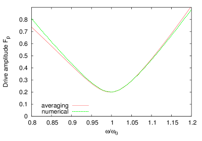
Figure 1: (color online) Comparison between numerical and averaging method predictions for the boundary of the first instability zone of the damped parametrically-driven oscillator of Eq. (1). In the region above the green line lies the unstable zone obtained by numerical computation, while the region above the red line is the analytical prediction for the unstable zone. The numerical results are obtained by numerically calculating the corresponding Floquet multipliers, when at least one of them has modulus equal to 1. The averaging predictions are given by Eq. (14). The fixed parameters of the equations of motion are $\gamma=0.1,\omega_{0}=1.0$. These parameters were also used to obtain the results portrayed in the remaining figures.

This result is valid for $\omega\approx\omega_{0}$ even in the presence of added noise. In Fig. (1) we find very good agreement between results obtained from numerical integration of Eq. (1) and the boundary given by the averaging technique.

We now will investigate the effect of added thermal noise on the parametric amplification mechanism rugar91 ; difilippo92prl ; natarajan95prl ; almog2007noise . We start by adding noise to Eq.(1) and obtain

$$\ddot{x}=-\omega^{2}_{0}x-\gamma\dot{x}+F_{p}\cos(2\omega t)\;x+R(t),$$ (15)

where $R(t)$ is a random function that satisfies the statistical averages $\langle R(t)\rangle=0$ and $\langle R(t)R(t^{\prime})\rangle=2T\gamma\delta(t-t^{\prime})$, according to the fluctuation-dissipation theorem kubo66 . $T$ is the temperature of the heat bath in which the oscillator (or resonator) is embedded. Once we integrate these equations of motion we can show how classical mechanical noise squeezing, heating, and cooling occur. We now summarize the method developed in batista2011cooling to analytically study the parametrically-driven oscillator with added noise, as given by Eq. (15).

II.1 Green’s function method

The equation for the Green’s function of the parametrically-driven oscillator is given by

$$\left[\frac{\partial^{2}}{\partial t^{2}}+\omega_{0}^{2}+\gamma\frac{\partial}{\partial t}-F_{p}\cos(2\omega t)\right]\;G(t,t^{\prime})=\delta(t-t^{\prime}).$$ (16)

Since we are interested in the stable zones of the parametric oscillator, for $t<t^{\prime}$ $G(t,t^{\prime})=0$ and by integrating the above equation near $t=t^{\prime}$, we obtain the initial conditions when $t=t^{\prime}+0^{+}$, $G(t,t^{\prime})=0$ and $\frac{\partial}{\partial t}G(t,t^{\prime})=1.0$. Using the Green’s function we obtain the solution $x(t)$ of Eq. (15) in the presence of noise $R(t)$

$$x(t) =x_{h}(t)+\int_{-\infty}^{\infty}dt^{\prime}\;G(t,t^{\prime})R(t^{\prime}),$$ (17)

$$\dot{x}(t) =v(t)=v_{h}(t)+\int_{-\infty}^{\infty}dt^{\prime}\;\frac{\partial}{\partial t}G(t,t^{\prime})R(t^{\prime}),$$ (18)

where $x_{h}(t)$ is the homogeneous solution, which in the stable zone decays exponentially with time; since we assume the pump has been turned on for a long time, $x_{h}(t)=0$. By statistically averaging the fluctuations as a function of time we obtain

$$\langle x^{2}(t)\rangle = \iint_{-\infty}^{\infty}dt^{\prime}\;dt^{\prime\prime}G(t,t^{\prime})G(t,t^{\prime\prime})\langle R(t^{\prime})R(t^{\prime\prime})\rangle=2T\gamma\int_{0}^{\infty}d\tau\;G(t,t-\tau)^{2},$$ (19)

$$\langle v^{2}(t)\rangle = 2T\gamma\int_{-\infty}^{t}dt^{\prime}\;\left[\frac{\partial}{\partial t}G(t,t^{\prime})\right]^{2}$$ (20)

$$= \omega^{2}_{0}\langle x^{2}(t)\rangle-2F_{p}\gamma T\int^{\infty}_{0}d\tau\cos(2\omega(t-\tau))\;G(t-\tau,t)^{2}.$$

where $\tau=t-t^{\prime}$.

Although equation (15) may be solved exactly by using Floquet theory and Green’s functions methods wies85 , one obtains very complex solutions. Instead, we find fairly simple analytical approximations to the Green’s functions and, subsequently, to the statistical averages of fluctuations using the averaging method. We then use the solution of the system of coupled differential equations (13), where the initial conditions at $t=t^{\prime}$ are given by $u(t^{\prime})=-\sin(\omega t^{\prime})/\omega$ and $v(t^{\prime})=-\cos(\omega t^{\prime})/\omega$ and obtain the approximate Green’s function is

$$G(t,t^{\prime})\approx-\frac{e^{-\gamma(t-t^{\prime})/2}}{\omega}\left[\cos(\omega t)\left(\cosh(\kappa\,(t-t^{\prime}))\sin(\omega t^{\prime})+\frac{\beta-\delta}{\kappa}\sinh(\kappa\,(t-t^{\prime}))\cos(\omega t^{\prime})\right)\right.$$

$$\left.-\sin(\omega t)\left(\frac{\beta+\delta}{\kappa}\sinh(\kappa\,(t-t^{\prime}))\sin(\omega t^{\prime})+\cosh(\kappa\,(t-t^{\prime}))\cos(\omega t^{\prime})\right)\right],$$ (21)

for $t>t^{\prime}$ and $G(t,t^{\prime})=0$ for $t<t^{\prime}$. In the stable zone of the parametrically-driven oscillator, when $|\beta|>|\delta|$ , we can rewrite the Green’s function replacing the initial conditions and using simplifying trigonometrical identities. The change of variables $t^{\prime}=t-\tau$ leads to

$$G(t,t-\tau)\approx\frac{e^{-\gamma\tau/2}}{\omega}\left\{\cosh(\kappa\,\tau)\sin(\omega\tau)+\frac{\delta}{\kappa}\sinh(\kappa\,\tau)\cos(\omega\tau)\right.$$

$$\left.-\frac{\beta}{\kappa}\sinh(\kappa\,\tau)\left[\cos(\omega\tau)\cos(2\omega t)+\sin(\omega\tau)\sin(2\omega t)\right]\right\}.$$ (22)

We notice that by varying the pump amplitude $F_{p}$ and the detuning $\Omega$, we can create a continuous family of classical thermo-mechanical squeezed states, generalizing the experimental results of Rugar and Grütter rugar91 . An estimate of the time average of the thermal fluctuations, when $|\beta|>|\delta|$, is given by

$$\overline{\langle x^{2}(t)\rangle} = \frac{2T\gamma}{\omega^{2}}\int_{0}^{\infty}e^{-\gamma\tau}\left\{\left[\cosh(\kappa\tau)\sin(\omega\tau)+\frac{\delta}{\kappa}\sinh(\kappa\tau)\cos(\omega\tau)\right]^{2}+\frac{\beta^{2}}{2\kappa^{2}}\sinh^{2}(\kappa\tau)\right\}\,d\tau$$ (23)

$$= \frac{2T\gamma}{\omega^{2}}\left[I_{1}+I_{2}+\delta^{2}I_{3}+\delta I_{4}\right],$$

where the integrals are given by

$$I_{1} = \frac{\beta^{2}}{2\kappa^{2}}\int_{0}^{\infty}e^{-\gamma\tau}\sinh^{2}(\kappa\tau)d\tau=\frac{\beta^{2}}{\gamma(\gamma^{2}-4\kappa^{2})},$$

$$I_{2} = \int_{0}^{\infty}e^{-\gamma\tau}\cosh^{2}(\kappa\tau)\sin^{2}(\omega\tau)d\tau$$

$$= \frac{1}{2}\left\{\frac{1}{2\gamma}-\frac{\gamma}{2(\gamma^{2}+4\omega^{2})}+\frac{\gamma}{2(\gamma^{2}-4\kappa^{2})}-\frac{1}{4}\mbox{Re}\left[\frac{1}{\gamma-2\kappa-2i\omega}+\frac{1}{\gamma+2\kappa-2i\omega}\right]\right\},$$

$$I_{3} = \frac{1}{\kappa^{2}}\int_{0}^{\infty}e^{-\gamma\tau}\sinh^{2}(\kappa\tau)\cos^{2}(\omega\tau)d\tau$$

$$= \frac{1}{\kappa^{2}}\left\{\frac{\kappa^{2}}{\gamma(\gamma^{2}-4\kappa^{2})}+\frac{1}{8}\mbox{Re}\left[\frac{1}{\gamma-2\kappa-2i\omega}+\frac{1}{\gamma+2\kappa-2i\omega}\right]-\frac{\gamma}{4(\gamma^{2}+4\omega^{2})}\right\},$$

$$I_{4} = \frac{1}{2\kappa}\int_{0}^{\infty}e^{-\gamma\tau}\sinh(2\kappa\tau)\sin(2\omega\tau)d\tau=\frac{1}{4}\mbox{Im}\left[\frac{1}{\kappa(\gamma-2\kappa-2i\omega)}-\frac{1}{\kappa(\gamma+2\kappa-2i\omega)}\right].$$

A time-averaged estimate of the statistically averaged thermal fluctuations in velocity, when $|\beta|>|\delta|$, is given by

$$\overline{\langle v^{2}(t)\rangle} = \omega^{2}_{0}\overline{\langle x^{2}(t)\rangle}+\frac{4F_{p}T\beta}{\kappa}\int^{\infty}_{0}d\tau\,e^{-\gamma\tau}\sinh(\kappa\,\tau)\left[\cosh(\kappa\,\tau)\sin(\omega\tau)+\frac{\delta}{\kappa}\sinh(\kappa\,\tau)\cos(\omega\tau)\right]\times$$ (24)

$$\overline{\cos(2\omega(t-\tau))\left[\cos(2\omega(t-\tau))\cos(\omega\tau)+\sin(2\omega(t-\tau))\sin(\omega\tau)\right]}$$

$$= \omega^{2}_{0}\overline{\langle x^{2}(t)\rangle}-8\omega T\beta^{2}(\delta I_{3}+I_{4}).$$

An estimate of the statistically averaged thermal fluctuations, when $|\beta|>|\delta|$, is given by

$$\langle x^{2}(t)\rangle \approx \overline{\langle x^{2}(t)\rangle}+A_{2\omega}\cos(2\omega t)+B_{2\omega}\sin(2\omega t)+A_{4\omega}\cos(4\omega t)+B_{4\omega}\sin(4\omega t),$$ (25)

where

$$A_{2\omega} = -\frac{4\beta T\gamma}{\omega^{2}}(K_{1}+K_{2}),$$

$$B_{2\omega} = -\frac{4\beta T\gamma}{\omega^{2}}(K_{3}+K_{4}),$$

with

$$K_{1} = \frac{1}{8}\mbox{Im}\left[\frac{1}{\kappa(\gamma-2\kappa-2i\omega)}-\frac{1}{\kappa(\gamma+2\kappa-2i\omega)}\right],$$

$$K_{2} = \frac{\delta}{\kappa^{2}}\left\{\frac{\kappa^{2}}{\gamma(\gamma^{2}-4\kappa^{2})}-\frac{\gamma}{4(\gamma^{2}+4\omega^{2})}+\frac{1}{8}\mbox{Re}\left[\frac{1}{\gamma-2\kappa-2i\omega}+\frac{1}{\gamma+2\kappa-2i\omega}\right]\right\},$$

$$K_{3} = \frac{1}{8\kappa}\left[\frac{4\kappa}{(\gamma^{2}-4\kappa^{2})}+\mbox{Re}\left(\frac{1}{\gamma-2\kappa-2i\omega}-\frac{1}{\gamma+2\kappa-2i\omega}\right)\right],$$

$$K_{4} = \frac{\delta}{8\kappa^{2}}\mbox{Im}\left[\frac{1}{\gamma-2\kappa-2i\omega}+\frac{1}{\gamma+2\kappa-2i\omega}-\frac{2}{\gamma-2i\omega}\right]$$

$$= \frac{\delta\omega}{4\kappa^{2}}\left[\frac{1}{(\gamma+2\kappa)^{2}+4\omega^{2}}+\frac{1}{(\gamma-2\kappa)^{2}+4\omega^{2}}-\frac{2}{\gamma^{2}+4\omega^{2}}\right].$$

The remaining coefficients of eq. (25) are given by

$$A_{4\omega} = \frac{\beta^{2}T\gamma}{4\omega^{2}\kappa^{2}}\mbox{Re}\left[\frac{1}{\gamma-2\kappa-2i\omega}+\frac{1}{\gamma+2\kappa-2i\omega}-\frac{2}{\gamma-2i\omega}\right],$$

$$B_{4\omega} = \frac{\beta^{2}T\gamma}{4\omega\kappa^{2}}\mbox{Im}\left[\frac{1}{\gamma-2\kappa-2i\omega}+\frac{1}{\gamma+2\kappa-2i\omega}-\frac{2}{\gamma-2i\omega}\right].$$

Notice that when one gets close to the zone of instability we obtain a far simpler expression for the average fluctuations. It is given approximately by

$$\langle x^{2}(t)\rangle\approx\frac{2T}{\omega^{2}}\left[\beta^{2}+\frac{\gamma^{2}}{4}+\delta^{2}\right]\frac{1}{\gamma^{2}-4\kappa^{2}}-\frac{4\beta T\gamma}{\omega^{2}(\gamma^{2}-4\kappa^{2})}\left[\frac{\delta}{\gamma}\cos(2\omega t)+\frac{1}{2}\sin(2\omega t)\right]$$ (26)

III Linear parametric amplification

In this section we study the parametric amplification of an added ac signal near the onset of the first instability zone of Matthieu’s equation. The equation is given by

$$\ddot{x}+\omega^{2}x=-\Omega x-\gamma\dot{x}+F_{p}\cos(2\omega t)\;x+F_{0}\cos(\omega t+\phi).$$ (27)

After doing averaging we obtain

$$\left(\begin{array}[]{c}\dot{u}\\ \dot{v}\end{array}\right)=-\frac{1}{2\omega}\left[\begin{array}[]{cc}\gamma\omega&\Omega+\frac{F_{p}}{2}\\ -\Omega+\frac{F_{p}}{2}&\gamma\omega\end{array}\right]\left(\begin{array}[]{c}u\\ v\end{array}\right)+\frac{F_{0}}{2\omega}\left(\begin{array}[]{c}\sin\phi\\ -\cos\phi\end{array}\right)$$ (28)

The fixed points are given by

$$\left(\begin{array}[]{c}u^{*}\\ v^{*}\end{array}\right)=\frac{F_{0}}{\gamma^{2}\omega^{2}+\Omega^{2}-F_{p}^{2}/4}\left[\begin{array}[]{cc}\gamma\omega&-\left(\Omega+\frac{F_{p}}{2}\right)\\ \Omega-\frac{F_{p}}{2}&\gamma\omega\end{array}\right]\left(\begin{array}[]{c}\sin\phi\\ -\cos\phi\end{array}\right)$$

$$\left(\begin{array}[]{c}u^{*}\\ v^{*}\end{array}\right)=\frac{F_{0}}{\gamma^{2}\omega^{2}+\Omega^{2}-F_{p}^{2}/4}\left(\begin{array}[]{c}\gamma\omega\sin\phi+(\Omega+F_{p}/2)\cos\phi\\ (\Omega-F_{p}/2)\sin\phi-\gamma\omega\cos\phi\end{array}\right)$$ (29)

The gain of the amplifier is defined in almog06 as

$$G(\phi) = 20\log\left|\frac{X_{\mbox{pump on}}}{X_{\mbox{pump off}}}\right|$$

$$= 10\log\left\{\frac{\left[(\gamma\omega)^{2}+\Omega^{2}+F_{p}^{2}/4+F_{p}\left[\Omega\cos(2\phi)+\gamma\omega\sin(2\phi)\right]\right](\gamma^{2}\omega^{2}+\Omega^{2})}{(\gamma^{2}\omega^{2}+\Omega^{2}-F_{p}^{2}/4)^{2}}\right\},$$

where $\left|X\right|=\sqrt{u^{*2}+v^{*2}}$ and the pump off means $F_{p}=0$. Rugar and Grütter rugar91 have studied this amplification process experimentally and also analytically via a perturbative method described by Louisell louis60 . Although, their results agreed well with their experimental data, we believe that we can increase the applicability of mechanical parametric amplification of small signals by applying the averaging method and allowing for detuning. We also compare our analytical estimates of gain to the gain obtained from a full numerical integration of the equations of motion (27). The numerical gain is given by the expression in Eq. (III) with the analytical fixed-point values replaced by the numerical fixed points of the first-return Poincaré map obtained from the integration of Eq. (27) after transients died out, i.e. $x(nT)^{2}+y(nT)^{2}/\omega^{2}$, where $T=\pi/\omega$ and $n>>1$.

IV Signal to noise ratio

Following the previous definition of gain, we define a measure of the SNR as

$$SNR_{0}=10\log\left(\frac{u^{*2}+v^{*2}}{\overline{\langle x^{2}\rangle}}\right),$$ (31)

where the fixed points $u^{*}$ and $v^{*}$ are given by Eq. (29) and the time-averaged thermal fluctuations $\overline{\langle x^{2}\rangle}$ are given by Eq. (23). Near the first instability zone we can write down this expression, with the help of Eq. (26), approximately as

$$SNR_{0}=10\log\left\{\frac{2F_{0}^{2}\omega^{2}}{T(\gamma^{2}\omega^{2}+\Omega^{2}-F_{p}^{2}/4)}\left[1+\frac{F_{p}\left[\Omega\cos(2\phi)+\gamma\omega\sin(2\phi)\right]}{(\gamma\omega)^{2}+\Omega^{2}+F_{p}^{2}/4}\right]\right\}$$ (32)

Another measure of the SNR is given by comparing the signal intensity with the noise level at the same frequency, that is at $2\omega$. This is given by the expression

$$SNR_{2\omega}=10\log\left(\frac{u^{*2}+v^{*2}}{\sqrt{|A_{2\omega}|^{2}+|B_{2\omega}|^{2}}}\right),$$ (33)

where the coefficients $A_{2\omega}$ and $B_{2\omega}$ are defined in Eq. (25). By dimensional analysis one notices that $A_{2\omega}$ and $B_{2\omega}$ have the same dimensional units as $u^{*2}$ and $v^{*2}$. Near the first instability zone we obtain a simple estimate for this SNR measure, namely

$$SNR_{2\omega}=10\log\left\{\frac{F_{0}^{2}\omega^{2}}{2|F_{p}|T(\gamma^{2}\omega^{2}+\Omega^{2}-F_{p}^{2}/4)}\left[\frac{(\gamma\omega)^{2}+\Omega^{2}+F_{p}^{2}/4+F_{p}\left[\Omega\cos(2\phi)+\gamma\omega\sin(2\phi)\right]}{\sqrt{\Omega^{2}+\gamma^{2}\omega^{2}}}\right]\right\}$$ (34)

V Results and discussion

In Fig. (2) we plot the Green’s functions obtained directly from the numerical integration of Eq. (16) alongside analytical approximation results given by Eq. (21), if $|\beta|>|\delta|$, or by Eq. (22) if $|\beta|<|\delta|$. We obtain excellent agreement between the two methods, what implies that our analytical estimates of $\langle x^{2}(t)\rangle$ are accurate. The numerical integration was performed using a RK4 algorithm with a time step given by $\pi/(512\omega)$.

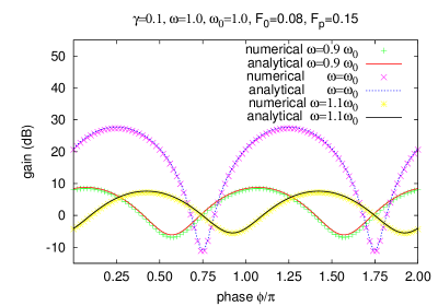
Figure 3: Comparison between numerical and analytical estimates of gain as a function of phase. The analytical gain is given by Eq. (III). The numerical values are given by the expression in Eq. (III) with the analytical fixed-point values replaced by the numerical fixed points of the first-return Poincaré map obtained from the integration of Eq. (27) after transients died out and in accordance with the transformation in Eq. (2). Observe that both gain and absorption are reduced with detuning.

In Fig. (3) we obtain excellent fitting between analytical results for gain obtained by the averaging method in Eq. (III) and numerical results given by the fixed point of the first-return Poincaré map of Eq. (27) obtained from the integration after transients died out.

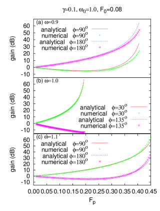
Figure 4: Comparison between numerical and analytical estimates of gain as a function of pump amplitude $F_{p}$. The analytical gain is given by Eq. (III). The numerical values are given by the expression in Eq. (III) with the analytical fixed-point values replaced by the numerical fixed points of the first-return Poincaré map obtained from the integration of Eq. (27) after transients died out.

In Fig. (4) a comparison between numerical and analytical estimates of gain as a function of pump amplitude $F_{p}$ is shown. Tow different values of phase are depicted. One observes a very strong dependance on phase between the pump and the external additive drive. One should obtain a divergence in gain as the boundary between stable and unstable response is reached. Again very good estimates are obtained.

In Fig. (5) we show a logarithmic plot of the dc component of the mean square displacement over the heat bath temperature. The steep rise of the curve as the pump amplitude is increased indicates that the noise is also amplified by the parametric oscillator.

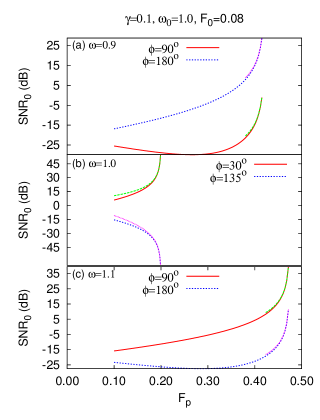
Figure 6: Plot of signal to noise ratio SNR₀ as defined in Eq. (31) along with corresponding approximations given by Eq. (32).

In Fig. (6) we show logarithmic plots of the amplitude of the signal (amplitude of response of the parametric oscillator due to the external ac drive) over the noise (here the dc component of the mean square displacement). Note that the simple estimates given by Eq. (32) give very good approximation as one gets close to the first instability zone in parameter space.

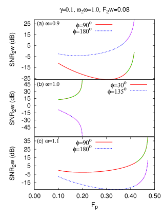
Figure 7: Plots of the signal to noise ratio SNR_2ω as defined in Eq. (33), in which the signal is given by $u^{*2}+v^{*2}$ and the noise is given by the amplitude of squeezing at $2\omega$ of the mean square displacement $\langle x^{2}(t)\rangle$ as given by $\sqrt{|A_{2\omega}|^{2}+|B_{2\omega}|^{2}}$, in which $A_{2\omega}$ and $B_{2\omega}$ are defined in Eq. (25). Very precise approximations are also plotted, given by Eq. (34)

In Fig. (7) we show logarithmic plots of the amplitude of the signal (amplitude of response of the parametric oscillator due to the external ac drive) over the average fluctuations amplitude that oscillate at frequency $2\omega$ (here the ac component of the mean square displacement).

VI Conclusion

The ability to reduce the influence of thermal noise in parametric amplifiers (which includes the linear regime of MEMS devices and optomechanical cavities), can greatly improve the accuracy and precision of measuring small masses and weak forces. Here we extended the theoretical work related to the seminal experimental research by Rugar and Grütter rugar91 . For a long time since its publication there has not appear in the literature a sound explanation based on stochastic dynamics of the essential features of the classical thermal noise squeezing phenomena observed there. Recently, though, one of the authors (A.A.B) has proposed a stochastic dynamics model batista2011cooling obtained by approximating the Green’s functions of the parametric oscillator using averaging techniques to account for the observed experimental effects. Here we extend this work and give analytical approximate results for SNR in parametric amplification. Here we propose two different kinds of SNR (SNR₀ and SNR_2ω). These estimates of SNR give a measure of the effectiveness of the parametric amplifiers in the presence additive noise. The analytical results presented here confirm, that in both measures of SNR, that the parametric amplifier is indeed a very good amplifier, with sensitive amplification dependant on frequency, on phase and with low noise. Further refinement of our results may be achieved by including more details about the noise model, such as memory effects grifoni98 ; batista08 , by taking into account the coupling to a heat bath that could be made out of photons, as in radiation-pressure cooling, or via coupling to phonons. Further improvements of the accuracy of the predictions should be obtained by taking nonlinear terms into account, especially when one gets close, in parameter space, to the first zone of instability. It is noteworthy to observe that our method may be applied to the linear response of nonlinear oscillators in the presence of both an ac drive and thermal noise.

Finally, we note that this model can also be applied to the dynamics of ions in quadrupole ion guides or traps paul90 or traps for neutral particles with magnetic dipole moments lovelace1985 . The presence of noise would indicate that the vacuum is not complete. One would obtain an estimate of the limits of mass spectroscopy in quadrupole ion guides, where the spectral limit is bounded by the ion guide length and the amount of noise present in the system.

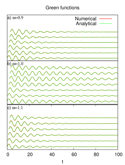
Figure 2: (color online) In the frames above we show several Green’s functions with equally-spaced in time initial conditions in one given period of the parametric driving. They are vertically spaced for clarity, since all asymptotes are zero. In each frame we have a comparison between numerical results given by the numerical integration of Eq. (16) and the analytical approximate results given by Eqs. (21) or (22). We have a) $\omega=0.9\,\omega_{0}$, b) $\omega=1.0\,\omega_{0}$, and c) $\omega=1.1\,\omega_{0}$. The initial values of the Green’s functions are $G(t,t^{\prime})=0$ and $\frac{\partial}{\partial t}G(t,t^{\prime})=1.0$ when $t=t^{\prime}+0^{+}$. The pump amplitude used was $F_{p}=0.15$.

Figure 5: (color online) Log plot of the dc component of the mean square displacement, $\overline{\langle x^{2}(t)\rangle}$, as given by Eqs. (23). In the linear parametric oscillator with thermal noise the temperature of the oscillator grows monotonically until it diverges at the boundary between stable and unstable zones. The approximating curves are given by Eq. (26).

References

- (1) M. Faraday, Philos. Trans. R. Soc. London 121, 319 (1831)
- (2) L. Ruby, Am. J. Phys. 64, 39 (1996)
- (3) W. Paul, Rev. of Mod. Phys. 62, 531 (1990)
- (4) A. Dorsel, J. McCullen, P. Meystre, E. Vignes, and H. Walther, Phys. Rev. Lett. 51, 1550 (1983)
- (5) W. Dougherty, K. Bruland, J. Garbini, and J. Sidles, Meas. Sci. and Technol. 7, 1733 (1996)
- (6) M. Moreno-Moreno, A. Raman, J. Gomez-Herrero, and R. Reifenberger, Appl. Phys. Lett. 88, 193108 (2006), ISSN 0003-6951
- (7) M. Requa and K. Turner, Appl. Phys. Lett. 88, 263508 (2006)
- (8) K. Turner, S. Miller, P. Hartwell, N. MacDonald, S. Strogatz, and S. Adams, Nature 396, 149 (1998)
- (9) G. Binnig, C. Quate, and C. Gerber, Phys. Rev. Lett 56, 930 (1986)
- (10) D. Rugar and P. Grutter, Phys. Rev. Lett. 67, 699 (1991)
- (11) R. Almog, S. Zaitsev, O. Shtempluck, and E. Buks, Phys. Rev. Lett. 98, 78103 (2007)
- (12) L. Falk, Am. J. Phys. 47, 325 (1979)
- (13) Berthet, R. and Petrosyan, A. and B. Roman, Am. J. Phys. 70, 744 (2002)
- (14) P. Tien, J. of Appl. Phys. 29, 1347 (1958), ISSN 0021-8979
- (15) R. Landauer, J. of Appl. Phys. 31, 479 (1960), ISSN 0021-8979
- (16) W. H. Louisell, Coupled Mode and Parametric Electronics (Wiley, New York, 1960)
- (17) W. Lee and E. Afshari, IEEE Transactions on Circuits and Systems I: Regular Papers, 1(2011), ISSN 1549-8328
- (18) A. Cleland, New Journal of Physics 7, 235 (2005)
- (19) A. A. Batista, J. of Stat. Mech. (Theory and Experiment) 2011, P02007 (2011)
- (20) F. Verhulst, Nonlinear differential equations and dynamical systems (Springer-Verlag, New York, 1996)
- (21) J. Guckenheimer and P. Holmes, Nonlinear Oscillations, Dynamical Systems, and Bifurcations of Vector Fields (Springer-Verlag, New York, 1983)
- (22) F. DiFilippo, V. Natarajan, K. Boyce, and D. Pritchard, Phys. Rev. Lett. 68, 2859 (1992)
- (23) V. Natarajan, F. DiFilippo, and D. Pritchard, Phys. Rev. Lett. 74, 2855 (1995)
- (24) R. Kubo, Rep. Prog. Phys. 29, 255 (1966)
- (25) K. Wiesenfeld and B. McNamara, Phys. Rev. Lett. 55, 13 (1985)
- (26) R. Almog, S. Zaitsev, O. Shtempluck, and E. Buks, Appl. Phys. Lett. 88, 213509 (2006)
- (27) M. Grifoni and P. Hänggi, Phys. Rep. 304, 229 (1998)
- (28) A. A. Batista, F. A. Oliveira, and H. N. Nazareno, Phys. Rev. E 77, 066216 (2008)
- (29) R. Lovelace, C. Mehanian, T. Tommila, and D. Lee, Nature 318, 30 (1985)