Semi-relativistic effects in spin-1/2 quantum plasmas

Abstract

Emerging possibilities for creating and studying novel plasma regimes, e.g. relativistic plasmas and dense systems, in a controlled laboratory environment also requires new modeling tools for such systems. This brings motivation for theoretical studies of the kinetic theory governing the dynamics of plasmas for which both relativistic and quantum effects occur simultaneously. Here, we investigate relativistic corrections to the Pauli Hamiltonian in the context of a scalar kinetic theory for spin-$1/2$ quantum plasmas. In particular, we formulate a quantum kinetic theory that takes such effects as spin-orbit coupling and Zitterbewegung into account for the collective motion of electrons. We discuss the implications and possible applications of our findings.

I Introduction

Plasmas, in their full generality, make up a highly complex class of physical systems, from classical tenuous plasmas, in e.g. fluorescent lighting, to dense, strongly coupled systems, such as QCD plasmas. The large span of plasma systems implies that a wide variety of theoretical methods have been developed for their treatment. Even so, there are general principles that remain as common features between the different plasma systems. Therefore, methods used for one plasma system can in some cases be transferred to another plasma type, sometimes leading to new insights. One such example is the transferal of techniques for treating nonlinearities in classical plasmas to quantum mechanical plasmas. The latter, often termed quantum plasmas (see, e.g., Refs. Pines ; Manfredi ; Melrose ; Shukla-Eliasson ), to lowest order contains corrections due to the classical regime in terms of nonlocal terms, related to the tunneling aspects of the electron (in quantum plasmas, the ions are most often treated classically). Such tunneling effects can be incorporated in both kinetic and fluid descriptions of the collective electron motion Markowich-etal ; Haas-etal . Such collective tunneling effects may, e.g., lead to nanoscale limitations in plasmonic devices Marklund-etal and bound states near moving test charges in plasmas Else-etal . Another mean-field effect that may be added to the dynamics of classical plasmas concerns the electron spin, i.e. the possibility of large-scale magnetization of plasmas Marklund-Brodin . Such magnetization switching is known to be able to give new non-trivial features, such as metamaterial properties, allowing for, e.g., new soliton modes Pendry ; Brodin-Marklund . Moreover, the inclusion of the electron spin into the collective dynamics can be done either through a fluid or a kinetic approach Zamanian-etal . Furthermore, the inclusion of spin into the dynamics of a quantum plasma points in the direction of relativistic effects in such plasma systems, e.g. collective spin-orbit coupling. It is the intention of the present work to extend previous work into the weakly relativistic regime.

As indicated above, the dynamics of plasmas under extreme conditions is an important and integral part at many current and up-coming experimental facilities, and such investigations therefore constitutes a highly active research field. In particular, laboratory plasmas, such as laser generated plasmas, are currently presenting the possibility of studying previously unattainable plasma density regimes. It is well-known that in the high-density regime glenzer-redmer quantum effects start to play a role for, e.g., the dispersive properties of plasma waves neumayer ; fustlin ; glenzer . In nature, such dense relativistic plasmas can be found in planetary interiors and in stars Ichimaru . Moreover, relativistic contributions to such plasma dynamics are under many circumstances very important ross . Thus, when the parameters takes values characteristic for the quantum relativistic regime, one needs to consider more complex dynamical models in order to obtain accurate descriptions of a host of phenomena. A canonical starting point for dealing with high-density effects in a perturbative relativistic regime is offered by the quantum kinetic approach, here based on the Dirac description. Effects that can be included in such a perturbative model includes, e.g., spin dynamics, spin-orbit coupling, and Zitterbewegung. These examples have close connections to the nonperturbative relativistic quantum regime, in which e.g. pair production Nerush-etal ; Hebenstreit-etal1 ; Hebenstreit-etal2 ; Elkina-etal and other nonlinear quantum vacuum effects Marklund-Shukla become pronounced

Dense plasmas, and in particular short-time scale phenomena therein, have been successfully studied using Green’s functions techniques, such as the Kadanoff-Baym kinetic equations Kadanoff-Baym (see also Refs. Zwanzig ; Prigogine ; Barwinkel ; Klimontovich for similar approaches, and Ref. Kremp-etal for an overview and examples from femtosecond laser physics). Although the Kadanoff-Baym equations and similar indeed gives ample opportunity to treat a wide variety of systems, their generality also makes simplifying assumptions necessary, and under certain circumstances a mean-field model, that still retains memory effects and non-local structures, can be an adequate approximation Ichimaru . In particular the mean-field approach is well suited outside the regime of strong coupling effects. Here, we will be interested in phenomena in plasmas that are not strongly coupled, but still in regimes where a classical plasma descriptions is not fully adequate. Here we stress that a large number of different dimensionless parameters (see e.g. Refs. BMM-2008 ; Lundin2010 for more complete discussions) is needed to give a thorough description of  various plasma regimes. However, much insight can be gained by considering a simple density-temperature plot. In Figure 1 a schematic view of the parameter regime of interest for our study is presented, adopted from Ref. zamanian

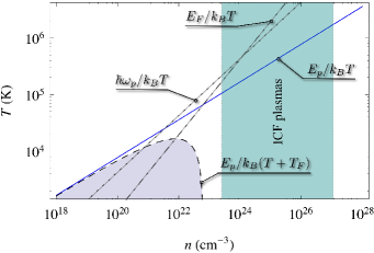
Figure 1: Different plasma regimes in the temperature-density parameter space. The dotted line is where the strong coupling parameter $\Gamma=E_{p}/k_{B}T=1$, where $E_{p}$ is the potential energy due to the nearest neighbor. For higher densities the average kinetic energy of the particles is given by the Fermi energy $k_{B}T_{F}$ rather than the thermal energy and the strong coupling parameter must there be replaced by $\Gamma_{F}=E_{p}/k_{B}(T+T_{F})$. In this graph $\Gamma_{F}=1$ is illustrated by the dashed curve, and the strong coupling region (shaded) lies below this line. In this region higher order correlations has to be taken into account, and the mean-field description is not valid. For comparison, the lines $\hbar\omega_{p}/k_{B}T$ (dotted gray line), where $\hbar\omega_{p}$ is the plasmon energy, and $T_{F}/T$ (dotted-dashed gray line) are also plotted. These measure, respectively, the relative importance of wave function dispersion and the Fermi pressure. As a rough estimate, the quantum regime lies below these lines. The area marked ICF denote the regime of relevance for inertial confinement fusion experiments.

In Section II we recall the Foldy-Wouthuysen transformation for particles in external fields and as a result we obtain a semi-relativistic Hamiltonian. We then go on to define the scalar quasi-distribution function for spin-1/2 particles in Section III. In Section IV we then derive the corresponding evolution equation for the distribution function. The evolution equation clearly depicts the importance of the different terms of the relativistic expansion. A comparison of our results to previous studies is made, and we discuss the applicability of our equation as well as the interpretation of the variables involved. In Section V our theory is illustrated by means of two examples from linearized theory, and finally, in Section VI, our main conclusions are summarized.

II The high-order corrections

The Dirac Hamiltonian can be written in the form

$$\hat{H}=\hat{\beta}mc^{2}+\Omega_{e}+\Omega_{o}\,,$$ (1)

where we have the even ($\hat{\beta}\Omega_{e}=\Omega_{e}\hat{\beta}$) operator

$$\Omega_{e}=q\phi\,,$$ (2)

and the odd ($\hat{\beta}\Omega_{o}=-\Omega_{o}\hat{\beta}$) operator

$$\Omega_{o}=c\bm{\hat{\alpha}}\cdot\left(\hat{\mathbf{p}}-q\mathbf{A}\right)\,,$$ (3)

where $\hat{\beta}$ and $\bm{\hat{\alpha}}$ are the $4\times 4$ Dirac matrices, $m$ is the electron mass, $q$ is the charge ($q=-e$ for an electron), $c$ is the speed of light, $\hat{\mathbf{p}}$ is the momentum operator and $\phi$ and $\mathbf{A}$ are the scalar and vector potential, respectively.

The odd operators in the Dirac Hamiltonian couples the positive and negative energy states of the Dirac bi-spinor. For the purpose of obtaining a perturbative expansion in the parameter $E/mc^{2}$, where $E$ is the typical energy associated with the second and third term in (1), we assume that the first term in (1) is large compared to these terms. The consecutive application of the unitary Foldy–Wouthuysen (FW) foldy-wouthuysen transformation

$$\hat{H}\rightarrow\exp\left(\beta\Omega_{o}/2mc^{2}\right)\hat{H}\exp\left(-\beta\Omega_{o}/2mc^{2}\right)\,,$$ (4)

yields a new Hamiltonian of the form (1) in which the new odd operators are of the order $1/mc^{2}$. Performing this transformation $n$ times yields terms up to order $(mc^{2})^{-n}$. This gives a separation of the positive and negative energy states up to an arbitrary order $n$ in $1/mc^{2}$.

Applying this transformation four times gives the following Hamiltonian for positive energy states with only even operators strange

$$\hat{H} =mc^{2}+q\phi+\frac{1}{2m}\left(\hat{\mathbf{p}}-\frac{q}{c}\mathbf{A}\right)^{2}-\frac{q\hbar}{2mc}\bm{\sigma}\cdot\mathbf{B}+\frac{\hbar^{2}q}{8m^{2}c^{2}}\nabla\cdot\mathbf{E}$$

$$-\frac{\hbar q}{4m^{2}c^{2}}\bm{\sigma}\cdot\left[\mathbf{E}\times\left(\hat{\mathbf{p}}-\frac{q}{c}\mathbf{A}\right)\right]-\frac{i\hbar^{2}q}{8m^{2}c^{2}}\bm{\sigma}\cdot\nabla\times\mathbf{E}$$

$$+\frac{1}{8m^{3}c^{2}}\left(\hat{\mathbf{p}}-\frac{q}{c}\mathbf{A}\right)^{4}$$ (5)

where $\bm{\sigma}$ here denotes a vector containing the $2\times 2$ Pauli matrices, $\hbar$ is the reduced Planck constant, $q$ is the charge, $m$ is the mass, $\mathbf{B}$ and $\mathbf{E}$ are the magnetic and electric field and $\phi$ and $\mathbf{A}$ are the corresponding potentials in the Coulomb gauge. We see that the first four terms constitute the Pauli Hamiltonian, while the remaining terms are higher order corrections. In particular, the sixth and seventh terms together gives Thomas precession and spin-orbit coupling, while the fifth and eight terms are the Darwin term and the so called mass-velocity correction term, respectively.

In Eq. (5) as well as in the Dirac theory we started from, the value of the spin $g$-factor is exactly 2. When applying the resulting theory, in section V, we will use the QED corrected value of $g\simeq 2.00232$, however. In spite of the smallness of the modification it turns out that this correction is important, as the applications of our theory are very sensitive to the exact value of the $g$-factor. In fact, the sensitivity of the kinetic theory to the value of $g$ was seen already in Ref. brodin . This may suggest that for consistency, the Hamiltonian for QED-corrections should be added to Eq. (5). Such an approach would indeed modify the $g$-value to the desired one in the theory presented below, but the augmented Hamiltonian would also add several new terms in the evolution equation for the electrons. Those extra terms are at least smaller than those kept by a factor of the order $(g-2)$, however. Thus the main effect from QED in the regime of study is the modification of the value of the $g$-factor as compared to the Dirac theory. As a consequence, the contributions from QED (see e.g. Ref. Groot-book for QED-corrections to the Dirac Hamiltonian) besides modifying the $g$-value will not be included here.

III Gauge-invariant Stratonovich-Wigner function

The extended phase-space scalar kinetic model is obtained using the Hamiltonian (5). Following Ref. zamanian , we are able to construct a gauge invariant scalar kinetic theory using a density matrix description for a spin-1/2 particle.

The basis states are $|\mathbf{x},\alpha\rangle=|\mathbf{x}\rangle\otimes|\alpha\rangle$, where $|\mathbf{x}\rangle$ is a state with position $\mathbf{x}$ and $|\alpha\rangle$ is the state with spin-up $\alpha=1$ or spin-down $\alpha=2$. As a starting point of this model we use the spinor state $\psi\left(\mathbf{x},\alpha,t\right)=\langle\mathbf{x},\alpha|\psi\rangle$ which fulfill the dynamical equation $i\hbar\partial_{t}\psi\left(\mathbf{x},\alpha,t\right)=\hat{H}\psi\left(\mathbf{x},\alpha,t\right)$, with the Hamiltonian (5).

With the spinors, we can define the density matrix as

$$\rho_{\alpha\beta}\left(\mathbf{x},\mathbf{y},t\right)=\langle\mathbf{x},\alpha|\hat{\rho}|\mathbf{y},\beta\rangle=\sum_{i}p_{i}\psi_{i}\left(\mathbf{x},\alpha,t\right)\psi_{i}^{\dagger}\left(\mathbf{y},\beta,t\right)\,,$$ (6)

where $p_{i}$ is the probability to have a state ${\psi}_{i}$. The density matrix fulfills the von Neumann equation

$$i\hbar\frac{\partial\hat{\rho}}{\partial t}=\left[\hat{H},\hat{\rho}\right]\,.$$ (7)

Once the density matrix has been defined, we can define the Wigner-Stratonovich transform strato as

$$W_{\alpha\beta}(\mathbf{x},\mathbf{p},t)=\int\frac{d^{3}z}{(2\pi\hbar)^{3}}\exp\left[-\frac{i}{\hbar}\mathbf{z}\cdot\Phi\right]\rho_{\alpha\beta}\left(\mathbf{x}+\frac{\mathbf{z}}{2};\mathbf{x}-\frac{\mathbf{z}}{2},t\right)\,,$$ (8)

where the phase

$$\Phi=\mathbf{p}-\frac{q}{c}\int_{-1/2}^{1/2}d\eta\mathbf{A}\left(\mathbf{x}+\eta\mathbf{z},t\right)\,$$ (9)

is used to ensure gauge invariance of the resulting distribution function. The Wigner-Stratonovich transform has the property that it must to be taken separately for each component of the 2-by-2 density matrix.

Different approaches to construct a kinetic theory from the Wigner-Stratonovich transformation are discussed in Ref. zamanian . Following this reference we here define a scalar distribution function $f(\mathbf{x},\mathbf{p},\mathbf{s},t)$ in the extended phase-space Phase-space-Note where $\mathbf{s}$ is a vector of unit length. This distribution function satisfies that

$$f(\mathbf{x},\mathbf{s},t)=\int d^{3}pf(\mathbf{x},\mathbf{p},\mathbf{s},t)\,,$$ (10)

gives the probability to find the particle at position $\mathbf{x}$ with spin-up in the direction of $\mathbf{s}$, and

$$f(\mathbf{p},\mathbf{s},t)=\int d^{3}xf(\mathbf{x},\mathbf{p},\mathbf{s},t)\,,$$ (11)

gives the probability to find the particle with momentum $\mathbf{p}$ with spin-up in the direction of $\mathbf{s}$. Using the Wigner-Stratonovich transformation, the scalar distribution function will be defined as zamanian

$$f(\mathbf{x},\mathbf{p},\mathbf{s},t) =\frac{1}{4\pi}\sum_{\alpha,\beta=1}^{2}\left(1+\mathbf{s}\cdot\bm{\sigma}\right)_{\alpha\beta}W_{\beta\alpha}(\mathbf{x},\mathbf{p},t)$$

$$=\frac{1}{4\pi}\mathrm{tr}(1+\mathbf{s}\cdot\bm{\sigma})W(\mathbf{x},\mathbf{p},t),$$ (12)

where $\mathrm{tr}$ denotes the trace over the spin indices. We recall that the expectation value polarization density is now given by

$$\left\langle\bm{\sigma}\right\rangle(\mathbf{x},t)=\mathrm{tr}[\bm{\sigma}\rho(\mathbf{x},\mathbf{y},t)]=3\int d^{3}pd^{2}sf(\mathbf{x},\mathbf{p},\mathbf{s},t)\mathbf{s},$$ (13)

where we stress the need for the factor 3. This follows from the form of the transformation (12) and is needed to compensate for the quantum mechanical smearing of the distribution function in spin space. Furthermore, it should be stressed that the independent spin variable $\mathbf{s}$ constructed in (12) generates the rest frame expression for the spin. In our theory, which is only weakly relativistic, this has limited consequences. The relation between the rest frame spin $\mathbf{s}$, and the spatial part of a the spin four-vector $\mathbf{S}$ is given by $\mathbf{S=s}+[\gamma^{2}/(\gamma+1)](\mathbf{v\cdot s)v/}c^{2}$ Jackson , where the kinematic quantities (i.e. the gamma factor $\gamma$ and the velocity $\mathbf{v}$) can be expressed in terms of $\mathbf{p}$ and $\mathbf{s}$ (see below). Since our weakly relativistic theory presented here is only concerned with spin-dependent terms up to order $\mathbf{v/}c$, the difference between $\mathbf{S}$ and $\mathbf{s}$ may be overlooked for the most part, e.g. when computing the magnetization current density.

IV Evolution equation for the scalar distribution function

Using the above formalism we obtain a fully gauge invariant Vlasov-like evolution equation for charged particles. One of the most basic quantum effects is the tendency for the wave function to spread out. In the non-relativistic version of the theory zamanian this effect end up in operators $\sin(\hbar\nabla_{x}\cdot\nabla_{p})$ and $\cos(\hbar\nabla_{x}\cdot\nabla_{p})$ acting on the fields and the distribution function, where the operators can be defined through the trigonometric Taylor-expansions taylorexp-note . In our present theory we will view the spatial gradient operator $\nabla_{x}$ as a small parameter, and drop terms of order $\nabla_{x}^{3}$ or smaller, which means dropping particle dispersive effects, that are smaller by a factor of the order $\delta^{2}$ where $\delta$ is the characteristic de Broglie wavelength over the macroscopic scale length. The other approximation made is to only account for weakly relativistic effects, as described above. This implies that only terms up to first order in the velocity is kept, and that the gamma factor is put to unity. The evolution equation is found using the transformations (8) and (12) on the evolution equation (7), which together with the above given approximations results in

$$0 =\frac{\partial f}{\partial t}+\left\{\frac{\mathbf{p}}{m}+\frac{\mu}{2mc}\mathbf{E}\times\left(\mathbf{s}+\nabla_{s}\right)\right\}\cdot\nabla_{x}f$$

$$+q\left(\mathbf{E}+\frac{1}{c}\left\{\frac{\mathbf{p}}{m}+\frac{\mu}{2mc}\mathbf{E}\times\left(\mathbf{s}+\nabla_{s}\right)\right\}\times\mathbf{B}\right)\cdot\nabla_{p}f$$

$$+\frac{2\mu}{\hbar}\mathbf{s}\times\left(\mathbf{B}-\frac{\mathbf{p}\times\mathbf{E}}{2mc}\right)\cdot\nabla_{s}f$$

$$+\mu\left(\mathbf{s}+\nabla_{s}\right)\cdot\partial_{x}^{i}\left(\mathbf{B}-\frac{\mathbf{p}\times\mathbf{E}}{2mc}\right)\partial_{p}^{i}f-\frac{\hbar^{2}q}{8m^{2}c^{2}}\partial_{x}^{i}(\nabla\cdot\mathbf{E})\partial_{p}^{i}f\,,$$ (14)

where $\mathbf{p}$ is the momentum (which is related to the velocity through the spin; see below) and $\mu=\hbar q/2mc$ (or $\mu=g\hbar q/4mc$).

The evolution equation (14) has three new effects compared to the equation in Ref. zamanian for spin-$1/2$ particles. The first one is the Thomas precession effect where the previous theory zamanian is extended by the substitution $\mathbf{B}\rightarrow\mathbf{B}-\mathbf{p}\times\mathbf{E}/{2mc}$ in the fourth and fifth terms of Eq. (14) . This effect comes from the spin-orbit coupling contribution in Hamiltonian (5) and, therefore, it is directly coupled with the evolution of the spin. The second new effect is the last term which is associated to the Darwin term. This term introduces the Zitterbewegung effect of the electron, and is the only contribution proportional to $\hbar^{2}$. The third effect is seen in the velocity-momentum relation, which is highlighted in the second and third terms. In Eq. (14) the term in $\{\}$ brackets resembles a velocity which has been modified by the spin, which will be discussed in some detail below. Finally, we point out that the factor in front of $\nabla_{s}f$ in the third term is indeed given by $d\mathbf{s/}dt$ Jackson , i.e. the laboratory rate of change of the rest frame value of the spin. Thus we note that Eq. (14) is consistent with the interpretation of $\mathbf{s}$ as the rest frame variable for the spin.

Next we consider the relation between the velocity and momentum. In order to relate this variables we use the Heisenberg equation of motion for the velocity operator

$$\hat{\mathbf{v}}=\frac{1}{i\hbar}[\hat{\mathbf{x}},\hat{H}].$$ (15)

For the Hamiltonian (5) we then get

$$\hat{\mathbf{v}}=\frac{1}{m}\left(-i\hbar\nabla-\frac{q}{c}\mathbf{A}\right)-\frac{\mu}{2mc}\bm{\sigma}\times\mathbf{E},$$ (16)

where we have neglected the last term in the Hamiltonian to simplify the equation slightly, (see the discussion about the mass correction below). We now recall that the Wigner transformation for an operator is multiplied by a factor $(2\pi\hbar)^{3}$, as compared to the the Wigner transformation for the density matrix. Similarly, for the spin transformation, the transformation for operators comes with a factor 3. Taking this into account and calculating the Wigner and Q transformation of the operator above gives the final relation

$$\mathbf{v}=\mathbf{v}(\mathbf{x},\mathbf{p},\mathbf{s},t)=\frac{\mathbf{p}}{m}+\frac{3\mu}{2mc}\mathbf{E}\times\mathbf{s}.$$ (17)

This is the function in extended phase space, which can be used to calculate the average velocity and the current density of the plasma. An important question that arises is whether the current density based on the velocity (17) will give the free current density or if correspond to some other physical quantity, e.g. the total current density. This question is addressed below, where we calculate the energy conservation law of our system, which confirms that the velocity in Eq. (17) is indeed the variable corresponding to the free current density.

In a more general context, the relationship between the momentum and the velocity is nontrivial. E.g. the spin orbit coupling has been shown to arise as a Berry phase term mathur . For further discussion of this interesting topic see e.g. berard ; bliokh ; bliokh2 ; gosselin .

When obtaining the evolution equation (14), we have not considered the effect of the mass-velocity correction term in order to get a more transparent formalism. This term will only produce a correction of the form $\mathbf{p}/{m}\longrightarrow\mathbf{p}/{m}\,(1+\mathbf{p}^{2}/2m^{2}c^{2})$ in the second term. Although this term is of the same order in an expansion in $1/c$, as compared to other terms that have been kept, we will not consider it as the classical relativistic terms are already well-known. Instead we focus on the new effects introduced by the spin and the Zitterbewegung.

The dynamics of the distribution function given by the Vlasov equation (14) is in the mean field approximation coupled to the Maxwell equations in the form

$$\nabla\cdot\mathbf{E}=4\pi\rho_{T}\,,\qquad\nabla\times\mathbf{B}=\frac{\partial\mathbf{E}}{\partial t}+4\pi\mathbf{J}_{T}\,,$$ (18)

where the total charge density and total current density are given by

$$\rho_{T}=\rho_{F}+\nabla\cdot\mathbf{P}\,\qquad\mathbf{J}_{T}=\mathbf{J}_{F}+\nabla\times\mathbf{M}+\frac{\partial\mathbf{P}}{\partial t}\,.$$ (19)

In the above expressions, the free charge density is

$$\rho_{F}=q\int d\Omega f\,,$$ (20)

where $d\Omega=d^{3}vd^{2}s$ is the integration measure performed over the three velocity variables and the two spin degrees of freedom. The spin vector has a fixed unity length and it is thus convenient to use spherical coordinates $(\varphi_{s},\theta_{s})$ do describe it. The free current density is given by

$$\mathbf{J}_{F}=q\int d\Omega\left(\frac{\mathbf{p}}{m}+\frac{3\mu}{2mc}\,\mathbf{E}\times\mathbf{s}\right)f.$$ (21)

With these charge and current densities, the conservation of charge is obtained as from (14) to be $\partial_{t}\rho_{F}+\nabla\cdot\mathbf{J}_{F}=0$. Furthermore the magnetization $\mathbf{M}$ and the polarization $\mathbf{P}$ are both due to the spin and they are calculated respectively as

$$\mathbf{M}=3\mu\int d\Omega\mathbf{s}f$$ (22)

and

$$\mathbf{P}=-3\mu\int d\Omega\frac{\mathbf{s}\times\mathbf{p}}{2mc}f.$$ (23)

The system of Maxwell’s equations with the magnetization (22) and polarization (23) and free current density (21), together with our main equation (14), satisfies an energy conservation law of the form

$$\partial_{t}W+\nabla\cdot\mathbf{K}=0.$$ (24)

Here the total energy density $W$ is given by

$$W=\frac{1}{2}\left(|\mathbf{E}|^{2}+|\mathbf{B}|^{2}\right)+\int d\Omega\left(\frac{\mathbf{p}^{2}}{2m}-3\mu\mathbf{s}\cdot\mathbf{B}\right)f\,,$$ (25)

and the energy flux vector $\mathbf{K}$ is given by

$$\mathbf{K}=\mathbf{E}\times\left(\mathbf{B}-\mathbf{M}\right)+\int d\Omega\left(\frac{\mathbf{p}^{2}}{2m}+3\mu\left(\mathbf{B}-\frac{\mathbf{p}\times\mathbf{E}}{2mc}\right)\cdot\mathbf{s}\right)\mathbf{v}f\,.$$ (26)

Apparently the first terms in (25) constitute the electromagnetic field energy density, and the integral term is the combined kinetic and magnetic dipole energy density. The first term of (26) is the Poynting vector, whereas the latter represents the combined flux of kinetic energy density and magnetic dipole energy. This energy conservation equation is a generalization of previous results for semi-classical theories for spin-1/2 plasmas brodin . It should be noted that although the theory presented here contains approximation, e.g. due to the weakly relativistic assumptions, the conservation law (24) is an exact property of the presented model.

V Linearized theory

In the present section, we are going to study the influence of the spin-orbit coupling and of the Darwin term on linear wave propagation. For this purpose we linearize the evolution equation (14), where the variables are separated into equilibrium and perturbed quantities (using the subindices $0$ and $1$, respectively, to denote them). Thus, the distribution function will be $f=f_{0}+f_{1}$, and the electric and magnetic field could be written as $\mathbf{E}=\mathbf{E}_{1}$ and $\mathbf{B}=\mathbf{B}_{0}+\mathbf{B}_{1}$ respectively. The evolution equation to linear order becomes

$$\frac{\partial f_{1}}{\partial t} +\frac{\mathbf{p}}{m}\cdot\nabla_{x}f_{1}+\frac{q}{mc}\mathbf{p}\times\mathbf{B}_{0}\cdot\nabla_{p}f_{1}+\frac{2\mu}{\hbar}\mathbf{s}\times\mathbf{B}_{0}\cdot\nabla_{s}f_{1}+\mu\nabla_{xi}\left[\mathbf{B}_{0}\cdot(\mathbf{s}+\nabla_{s})\right]\nabla_{pi}f_{1}$$

$$=-q\mathbf{E}_{1}\cdot\nabla_{p}f_{0}-\frac{\mu}{2mc}\mathbf{E}_{1}\times\left(\mathbf{s}+\nabla_{s}\right)\cdot\nabla_{x}f_{0}-\frac{q}{mc}\mathbf{p}\times\mathbf{B}_{1}\cdot\nabla_{p}f_{0}-\mu\nabla_{xi}\left[\mathbf{B}_{1}\cdot(\mathbf{s}+\nabla_{s})\right]\nabla_{pi}f_{0}$$

$$+\frac{\mu}{2mc}\nabla_{xi}\left[(\mathbf{p}\times\mathbf{E}_{1})\cdot(\mathbf{s}+\nabla_{s})\right]\nabla_{pi}f_{0}-\frac{q\mu}{2mc^{2}}\left[\mathbf{E}_{1}\times(\mathbf{s}+\nabla_{s})\right]\times\mathbf{B}_{0}\cdot\nabla_{p}f_{0}-\frac{2\mu}{\hbar}\mathbf{s}\times\mathbf{B}_{1}\cdot\nabla_{s}f_{0}$$

$$+\frac{\mu}{\hbar mc}\mathbf{s}\times(\mathbf{p}\times\mathbf{E}_{1})\cdot\nabla_{s}f_{0}+\frac{\hbar^{2}q}{8m^{2}c^{2}}\nabla_{xi}(\nabla\cdot\mathbf{E}_{1})\nabla_{pi}f_{0}\,.$$ (27)

In the following, we only study electrostatic modes (e.g. $\mathbf{B}_{1}=0$ in (27)) propagating along $\mathbf{B}_{0}$, as this gives a good illustration of the contribution from the relativistic terms, that are due to the Zitterbewegung effect and the spin-orbit coupling.

V.1 Darwin term contribution

Firstly we want to focus on the effect associated with Zitterbewegung. The Zitterbewegung is a rapid oscillatory motion of the electron which implies that if an instantaneous measurement of its velocity is performed, the result is the speed of light. The amplitude of the oscillatory motion is $x_{osc}\sim\hbar/2mc$ strange , which means that the electron cannot be localized, but is rapidly oscillating in a volume of the order of the cube of the Compton wavelength. The Zitterbewegung is a quantum relativistic effect and it is related to particle-antiparticle nature of the Dirac theory and to the nature of the spin. At the present, there is a growing interest in the detection of effects as the Zitterbewegung gerri .

The effect of the Zitterbewegung of the electron is introduced in the last term of Eq. (27), the Darwin contribution, which represents the smeared out electrostatic potential field that the electron sees when it fluctuates over a distance $x_{osc}$.

For the sake of simplicity, we examine the dispersion relation of Langmuir waves in an unmagnetized plasma. In order to focus on the effects of the Darwin contribution, we consider a one-dimensional unperturbed momentum distribution and let $f_{0}\rightarrow$ $f_{0}(p_{z}^{2})\delta(p_{x})\delta(p_{y})$ (for a more realistic 3D-momentum distribution, even the electrostatic unmagnetized case couple to the spin terms, as we will see in the next section). The total distribution function will then have the form of $f(z,p_{z},t)=f_{0}(p_{z}^{2})+f_{1}(z,p_{z},t)\exp(ikz-i\omega t)$, where $f_{0}$ and $f_{1}$ are the equilibrium and the perturbed distribution functions respectively. Furthermore, we consider a homogeneous plasma an neglect the motion of the heavy ions. The perturbed electric field is longitudinal, i.e. $\mathbf{E}_{1}=\hat{z}E_{1}\exp(ikz-i\omega t)$. Using the evolution equation (27), the perturbed distribution function is then related to the electric field amplitude by

$$f_{1}=\frac{-iqE_{1}}{\omega-kp_{z}/m}\left(1+\frac{\hbar^{2}k^{2}}{8m^{2}c^{2}}\right)\frac{\partial f_{0}}{\partial p_{z}}\,.$$ (28)

Combining Eq. (28) with Poisson equation $\nabla\cdot\mathbf{E}_{1}=ikE_{1}=4\pi q\int d\Omega f_{1}$, we obtain the dispersion relation

$$1=\frac{\omega_{p}^{2}}{k^{2}}\left(1+\frac{\hbar^{2}k^{2}}{8m^{2}c^{2}}\right)\int_{-\infty}^{\infty}dp_{z}\frac{\widehat{f_{0}}}{\left(p_{z}/m-\omega/k\right)^{2}}\,$$ (29)

where the re-normalized distribution function $\widehat{f_{0}}$ fulfills$\int_{-\infty}^{\infty}dp_{z}$ $\widehat{f_{0}}=1$.  For phase velocities larger than than the characteristic spread in $p_{z}/m$, we can Taylor expand the denominator, and write the dispersion relation as

$$\omega^{2}=\omega_{p}^{2}\left(1+\frac{\hbar^{2}k^{2}}{8m^{2}c^{2}}\right)\left(1+\frac{k^{2}\left\langle p_{z}^{2}\right\rangle}{m^{2}\omega^{2}}\right)$$ (30)

where $\left\langle p_{z}^{2}\right\rangle=\int_{-\infty}^{\infty}dp_{z}p_{z}^{2}\widehat{f_{0}}$ is the average of the squared momentum. Here the Landau damping term has been dropped, since the resonance is assumed to lie in the tail of the distribution.

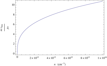
Figure 2: The parameter $mv_{\text{\rm Zitt}}/p_{F}$, relevant as a comparison when $T\rightarrow 0$, where $p_{F}$ is the Fermi momentum, is plotted as a function of density. This illustrates the relative importance of the Zitterbewegung and the Fermi momentum, i.e. the Fermi pressure, in the dispersion relation (31) above.

The term proportional to $\hbar^{2}k^{2}$ is the Zitterbewegung contribution to electrostatic modes. For not too large wave-numbers it is more significant than quantum contributions from the Bohm potential Manfredi that scales as $\hbar^{2}k^{4}$. Provided the wave-numbers are small, $\omega\simeq\omega_{p}$, and the dispersion relation can be further approximated as

$$\omega^{2}=\omega_{p}^{2}+k^{2}\left(\frac{\left\langle p_{z}^{2}\right\rangle}{m^{2}}+\frac{v_{\rm Zitt}^{2}}{2}\right)\,,$$ (31)

where $v_{\rm Zitt}=\hbar\omega_{p}/2mc$ can be understood as a velocity response of the plasma $v_{\rm Zitt}\sim x_{\rm osc}\omega_{p}$ to the rapid oscillations of the Zitterbewegung motion. The term $v_{\rm Zitt}^{2}k^{2}$ comes from the fact that the electron sees a smeared out electrostatic potential, and therefore, a gradient of the electric field and a force of the order $\hbar^{2}\nabla(\nabla\cdot\mathbf{E})/m^{2}c^{2}$. Similar to the effects of the Fermi pressure (which gives a non-zero $\left\langle p_{z}^{2}\right\rangle$ even when the temperature goes to zero) this implies a non-zero group velocity of the electron plasma waves even in the cold case (see also Fig. 2 for a comparison between the Fermi statistics and the Zitterbewegung, relevant for Eq. (31) when $T\rightarrow 0$). We note that the effect of the Darwin term related to Zitterbewegung becomes important for high-density plasmas when $\hbar\omega_{p}/mc^{2}$ is not too much smaller than unity.

V.2 Spin-orbit coupling contribution

The spin-orbit effect of Hamiltonian (5) appears as the Thomas precession correction (see e.g. Ref. Jackson-2 ) of the magnetic field in the fourth and fifth terms of Eq. (14).

Although this contribution can introduce interesting corrections to different types of wave modes, in this work we are going to follow the previous spirit and we analyze the quantum corrections to Langmuir waves, this time in a magnetized plasma. These modes have been studied previously in Ref. Petter in a phenomenological relativistic formalism where the appropriate Thomas precession factor of $1/2$ was not used. We consider again longitudinal electrostatic modes $\mathbf{E}_{1}=\hat{z}\,E_{1}\exp(ikz-i\omega t)$, but now propagating along an external magnetic field $\mathbf{B}_{0}=B_{0}\hat{z}$. As will be seen below, this will give an illustrative example of how the spin-orbit coupling modifies the usual dispersion relation. The distribution function will be taken to be of the form $f(z,\mathbf{p},\mathbf{s},t)=f_{0}(\mathbf{p}^{2},\theta_{s})+f_{1}(z,\mathbf{p},\mathbf{s},t)\exp(ikz-i\omega t)$. We use cylindrical coordinates for the momentum, i.e. $\mathbf{p}=\hat{x}p_{\perp}\cos\varphi_{p}+\hat{y}\mathbf{p}_{\perp}\sin\varphi_{\perp}+\hat{z}p_{z}$ with $\mathbf{p}^{2}=p_{\perp}^{2}+p_{z}^{2}$. Furthermore, we use spherical coordinates for the spin, i.e. $\mathbf{s}=\hat{x}\sin\theta_{s}\cos\varphi_{s}+\hat{y}\sin\theta_{s}\sin\varphi_{s}+\hat{z}\cos\theta_{s}$.

At first order, taking the Fourier analysis of the evolution equation (27), we have

$$\left(\frac{\partial}{\partial t}+\frac{\mathbf{p}}{m}\cdot\nabla_{x}-\omega_{c}\frac{\partial}{\partial\varphi_{p}}-\omega_{cg}\frac{\partial}{\partial\varphi_{s}}\right)f_{1} =-qE_{1}\left(1+\frac{\hbar^{2}k^{2}}{8m^{2}c^{2}}\right)\frac{\partial f_{0}}{\partial p_{z}}$$

$$-\frac{ik\mu p_{\perp}E_{1}}{2mc}\left(\sin\theta_{s}+\cos\theta_{s}\frac{\partial}{\partial\theta_{s}}\right)\left(\cos\varphi_{p}\sin\varphi_{s}-\sin\varphi_{p}\cos\varphi_{s}\right)\frac{\partial f_{0}}{\partial p_{z}}$$

$$+\frac{\mu}{\hbar mc}p_{\perp}E_{1}\left(\cos\varphi_{p}\cos\varphi_{s}+\sin\varphi_{p}\sin\varphi_{s}\right)\frac{\partial f_{0}}{\partial\theta_{s}}$$

$$-\frac{q\mu B_{0}E_{1}}{2mc^{2}}\left(\sin\theta_{s}\cos\varphi_{s}+\cos\theta_{s}\cos\varphi_{s}\frac{\partial}{\partial\theta_{s}}\right)\left(\cos\varphi_{p}\frac{\partial f_{0}}{\partial p_{\perp}}\right)$$

$$-\frac{q\mu B_{0}E_{1}}{2mc^{2}}\left(\sin\theta_{s}\sin\varphi_{s}+\cos\theta_{s}\sin\varphi_{s}\frac{\partial}{\partial\theta_{s}}\right)\left(\sin\varphi_{p}\frac{\partial f_{0}}{\partial p_{\perp}}\right)$$ (32)

where $\omega_{c}=qB_{0}/mc$ is the cyclotron frequency and $\omega_{cg}=(g/2)\omega_{c}$ is the spin precession frequency brodin . We note that the perturbed distribution function can be solved for in terms of the orthogonal eigenfunctions $\psi_{n}$ to the right hand side operator brodin ; Petter . Accordingly we make the expansion

$$f_{1}=\frac{1}{\sqrt{2\pi}}\sum_{n=-\infty}^{\infty}\sum_{n^{\prime}=-\infty}^{\infty}g_{n,n^{\prime}}(p_{\perp},p_{z},\theta_{s})\psi_{n}(p_{\perp},\varphi_{p})\exp(in^{\prime}\varphi_{s})\,,$$ (33)

where in general

$$\psi_{n}(p_{\perp},\varphi_{p}) = \frac{1}{\sqrt{2\pi}}\exp[-i(n\varphi_{v}-(k_{\perp}p_{\perp}/\omega_{c}m)\sin\varphi_{p})]$$ (34)

$$= \frac{1}{\sqrt{2\pi}}\sum_{n^{\prime\prime}=-\infty}^{\infty}J_{n^{\prime\prime}}\left(\frac{k_{\perp}p_{\perp}}{m\omega_{c}}\right)e^{i(n-n^{\prime\prime})\varphi_{p}}\,,$$ (35)

and $J_{n^{\prime\prime}}$ is the Bessel function. However, in this case for longitudinal mode with $k_{\perp}=0$, then

$$\psi_{n}(p_{\perp},\varphi_{p})=\frac{1}{\sqrt{2\pi}}e^{in\varphi_{p}}\,.$$ (36)

Using the distribution function (33) in Eq. (32), and then multiplying both sides by $\psi_{n}^{\ast}e^{-im\varphi_{s}}$ and integrating over $\varphi_{p}$ and $\varphi_{s}$, we find that the only terms that survive in the sum (33) are $g_{0,0}$ and $g_{\pm 1,\mp 1}$ zamanian ; brodin ; Petter . Thus, we find the solution for $f_{1}$ as

$$f_{1} =\left(\frac{-iqE_{1}(1+{\hbar^{2}k^{2}}/{8m^{2}c^{2}})}{\omega-kp_{z}/m}\right)\frac{\partial f_{0}}{\partial p_{z}}+\frac{i\mu p_{\perp}E_{1}}{2\hbar mc}\left[\frac{e^{i(\varphi_{p}-\varphi_{s})}}{\omega-\Delta\omega_{c}-kp_{z}/m}+\frac{e^{i(\varphi_{s}-\varphi_{p})}}{\omega+\Delta\omega_{c}-kp_{z}/m}\right]\frac{\partial f_{0}}{\partial\theta_{s}}$$

$$+\frac{ik\mu p_{\perp}E_{1}}{4mc}\left[\frac{e^{i(\varphi_{p}-\varphi_{s})}}{\omega-\Delta\omega_{c}-kp_{z}/m}-\frac{e^{i(\varphi_{s}-\varphi_{p})}}{\omega+\Delta\omega_{c}-kp_{z}/m}\right]\left(\sin\theta_{s}+\cos\theta_{s}\frac{\partial}{\partial\theta_{s}}\right)\frac{\partial f_{0}}{\partial\theta_{s}}\,,$$ (37)

where $\Delta\omega_{c}=\omega_{cg}-\omega_{c}$. The expression (37) is combined with

$$-i\omega E_{1}=-4\pi J_{Tz}\,,$$ (38)

is used to deduce the dispersion relation. Due to the dependence on the angles $\varphi_{s}$ and $\varphi_{p}$, the first term of (37) give raise to a free current density, whereas the other terms give raise to a polarization current density. The magnetization current density vanish identically. Combining (37) and (38) we find the dispersion relation

$$\omega =-\left(\omega_{p}^{2}+\frac{1}{2}v_{\rm Zitt}^{2}k^{2}\right)\int d\Omega p_{z}\frac{\frac{\partial\widehat{f_{0}}}{\partial p_{z}}}{\omega-kp_{z}/m}+\frac{6\pi^{3}\mu^{2}\omega}{\hbar m^{2}c^{2}}\int d\Omega p_{\perp}^{2}\frac{\widehat{f_{0}}}{\partial\theta_{s}}\sin\theta_{s}\left(\frac{1}{\omega-\Delta\omega_{c}-kp_{z}/m}-\frac{1}{\omega+\Delta\omega_{c}-kp_{z}/m}\right)$$

$$+\frac{3\mu^{2}\omega k\pi^{3}}{m^{2}c^{2}}\int d\Omega p_{\perp}^{2}\left(\sin\theta_{s}+\cos\theta_{s}\frac{\partial}{\partial\theta_{s}}\right)\frac{\partial\widehat{f_{0}}}{\partial p_{z}}\left(\frac{1}{\omega-\Delta\omega_{c}-kp_{z}/m}+\frac{1}{\omega+\Delta\omega_{c}-kp_{z}/m}\right)\,,$$ (39)

which is general for $\widehat{f_{0}}$ (where we have again used the distribution function re-normalized as $\int\widehat{f_{0}}d\Omega=1$).

As an example, let us examine an equilibrium distribution function with the form of a Maxwellian distribution and a spin dependent part zamanian

$$\widehat{f_{0}}(\mathbf{p}^{2},\theta_{s})=\frac{1}{N_{M}}e^{-\mathbf{p}^{2}/m^{2}v_{t}^{2}} \left[e^{\mu B_{0}/k_{B}T}(1+\cos\theta_{s})\right.$$

$$\left.+e^{-\mu B_{0}/k_{B}T}(1-\cos\theta_{s})\right]\,,$$ (40)

where $T$ is the temperature and $k_{B}$ is the Boltzmann constant, and the normalization factor is $N_{M}=4\pi(\pi m^{2}v_{t}^{2})^{3/2}\cosh(\mu B_{0}/k_{B}T)$. We note that the expression (40) is the thermodynamic equilibrium distribution for a plasma of moderate density where the magnitude of the chemical potential is large distribution-note .

To simplify the integrals we will consider the frequency range where the wave frequency $\omega$ be close to resonance with $\Delta\omega_{c}$. In this case, we neglect in (39) the terms with the denominators $1/(\omega+\Delta\omega_{c}-p_{z}k/m)$ because they are small compared with the terms with denominators $1/(\omega-\Delta\omega_{c}-p_{z}k/m)$. We are also going to take the limit when $\omega-\Delta\omega_{c}\gg p_{z}k/m$. Thus, using the equilibrium distribution function (40), Taylor expanding the denominators, neglecting the poles in $\omega=p_{z}k/m$ and $\omega-\Delta\omega_{c}=p_{z}k/m$, and integrating over $d\Omega$, we finally find the dispersion relation for Langmuir waves with spin-orbit coupling and Darwin effects

$$\omega^{2}\left\{1+\frac{\hbar^{2}\pi^{2}\omega_{p}^{2}}{8m^{2}c^{4}}\left[\frac{k^{2}v_{t}^{2}}{(\omega-\Delta\omega_{c})^{2}}+\frac{3k^{4}v_{t}^{4}}{2(\omega-\Delta\omega_{c})^{4}}\right]+\frac{\hbar\pi^{2}\omega_{p}^{2}v_{t}^{2}}{4mc^{4}}\tanh\left(\frac{\mu B_{0}}{k_{B}T}\right)\left[\frac{1}{\omega-\Delta\omega_{c}}+\frac{k^{2}v_{t}^{2}}{2(\omega-\Delta\omega_{c})^{3}}\right]\right\}$$

$$=\left(\omega_{p}^{2}+\frac{1}{2}v_{\rm Zitt}^{2}k^{2}\right)\left(1+\frac{3k^{2}v_{t}^{2}}{2\omega^{2}}\right)\,.$$ (41)

The coefficient in front of the terms with denominators $\propto\omega-\Delta\omega_{c}$ are typically small, except for very strong magnetic fields. Thus excluding the regime of an extremely strong external field, the frequency of the spin modes will be close to resonance, i.e. fulfill $\omega\simeq\Delta\omega_{c}$. More specifically, the deviation from exact resonance is of the order $\left(\omega-\Delta\omega_{c}\right)/\Delta\omega_{c}\sim(\hbar\Delta\omega_{c}/mc^{2})\tanh(\mu B_{0}/k_{B}T)$. We note that spin induced modes with $\omega\simeq\Delta\omega_{c}$ have already been found by Ref. brodin without the inclusion of spin-orbit coupling. However, it should be noted that the present wave mode is quite different from that previously found. In particular, the field is now completely electrostatic (whereas it was found to be completely electromagnetic in the previous case), and the present wave mode exists in the long wavelength regime, whereas the former wave mode brodin was dependent on a short wavelength, i.e. of the order of the electron gyroradius or shorter. Finally we note that even in the absence of an external magnetic field, a finite contribution from the electron spin remains, together with the Darwin contribution. In the absence of resonances we note that both these quantum contributions require a very high plasma density to be significant.

VI Conclusions

The starting point for our theory is the FW-transformation, applied on the Dirac equation, which is used to pick out the positive energy states. Using the Wigner-Stratonovich transformation (8) on the density matrix, together with a Q-transformation zamanian a scalar distribution function (12) can be defined. In the weakly relativistic limit, the evolution equation is given by (14) to leading order in the expansion parameters $\hbar L^{-1}/p$ and $\mu B/mc^{2}$, where $L$ is a characteristic macroscopic scale length, $p$ a characteristic momentum of particles, and $B$ a characteristic magnitude of the magnetic field. In addition to the magnetic dipole force and spin precession zamanian , which is included already in the Pauli Hamiltonian, Eq. (14)) also contains spin-orbit interaction, including the Thomas factor, and also the contribution from the Darwin term. A complication in the (weakly) relativistic theory that should be noted is the relation between momentum and velocity (17), which now is dependent on the spin variable. Moreover, when closing the system, the polarization (23) associated with the spin must be included in the current and charge density (19), and the expression for the free current density (21) is affected due to the aforementioned relation (17). It should also be stressed that the spin variable used to define $f(\mathbf{x},\mathbf{p},\mathbf{s},t)$ refers to the rest-frame spin, which is convenient, as two spherical angles for the spin variables is sufficient.

In order to illustrate the theory, we have presented examples of electrostatic interaction in magnetized and non-magnetized plasmas. By picking a 1-D unperturbed distribution function, the influence of the Darwin term, which is associated with Zitterbewegung, is highlighted in the case of a non-magnetized plasma. For a magnetized plasma, the spin-orbit terms leads to new types of resonances for electrostatic waves, which involve the combined effect of orbital and spin-precession motion.

The theory presented here is of most interest for systems where at least one of the parameters $\hbar\omega_{p}/mc^{2}$ or $\mu B/mc^{2}$ are not too small. Examples include e.g. laser-plasma interactions, astrophysical objects (e.g. white dwarf stars), solid state plasmas and strongly magnetized systems. The present paper is a first step to reach a fully relativistic quantum theory of plasmas.

- (1) D. Pines, J. Nucl. Energy, Part C Plasma Phys. 2, 5 (1961); D. Pines and J. R. Schrieffer, Phys. Rev. 124, 1387 (1961); D. Pines and J. R. Schrieffer, Phys. Rev. 125, 804 (1962); D. Pines, Elementary Excitations in Solids (W. A. Benjamin: N. Y., 1963).
- (2) G. Manfredi, Fields Inst. Commun. 46, 263 (2005). arXiv:quant-ph/0505004v1.
- (3) D. B. Melrose, Quantum Plasmadynamics: Unmagnetized Plasmas (New York: Springer, 2008).
- (4) P. K. Shukla and B. Eliasson, Physics Uspekhi 53, 51 (2010).
- (5) P. A. Markowich, C. A. Ringhofer, and C. Schmeiser, Semiconductor Equations (Springer-Verlag, 2002).
- (6) F. Haas, M. Marklund, G. Brodin, and J. Zamanian, Phys. Lett. A 374, 481 (2010); F Haas, J. Zamanian, M. Marklund, and G. Brodin, New J. Phys. 12, 073027 (2010).
- (7) M. Marklund, G. Brodin, L. Stenflo, and C. S. Liu, EPL 84,17006 (2008).
- (8) D. Else, R. Kompaneets, and S. V. Vladimirov, EPL 94, 35001 (2011).
- (9) M. Marklund and G. Brodin, Phys. Rev. Lett. 98, 025001 (2007)
- (10) D. R. Smith, J. B. Pendry, and M. C. K. Wiltshire, Science 305, 788 (2004); M. Marklund, P. K. Shukla, L. Stenflo, and G. Brodin, Phys. Lett. A 341, 231 (2005); M. Marklund, P. K. Shukla, and L. Stenflo, Phys. Rev. E 73, 037601 (2006).
- (11) G. Brodin and M. Marklund, New J. Phys. 10, 115031 (2008).
- (12) J. Zamanian, M. Stefan, M. Marklund, and G. Brodin, Phys. Plasmas 17, 102109 (2010).
- (13) S. H. Glenzer and R. Redmer, Rev. Mod. Phys. 81, 1625 (2009).
- (14) P. Neumayer et al., Phys. Rev. Lett. 105, 075003 (2010).
- (15) R. R. Fäustlin et al., Phys. Rev. Lett. 104, 125002 (2010).
- (16) S. H. Glenzer et al., Phys. Rev. Lett. 98, 065002 (2007).
- (17) S. Ichimaru, Statistical Plasma Physics, Volume II: Condensed Plasmas (Westview, Oxford, 2004).
- (18) J. S. Ross et al., Phys. Rev. Lett. 104, 105001 (2010).
- (19) E.N. Nerush, I.Yu.Kostyukov, A.M. Fedotov, N.B. Narozhny, N.V. Elkina, and H. Ruhl, Phys. Rev. Lett. 106, 035001 (2011).
- (20) F. Hebenstreit, R. Alkofer, G.V. Dunne, and H. Gies, Phys. Rev. Lett. 102, 150404 (2009).
- (21) F. Hebenstreit, A. Ilderton, M. Marklund, and J. Zamanian, Phys. Rev. D 83, 065007 (2011).
- (22) N.V. Elkina, A.M. Fedotov, I.Yu. Kostyukov, M.V. Legkov, N.B. Narozhny, E.N. Nerush, and H. Ruhl, Phys. Rev. ST Accel. Beams, 14, 054401 (2011).
- (23) M. Marklund and P. K. Shukla, Rev. Mod. Phys. 78, 591 (2006).
- (24) L.P. Kadanoff and G. Baym, Quantum Statistical Mechanics (Benjamin, New York, 1962).
- (25) R. Zwanzig, J. Chem. Phys. 33, 1338 (1960).
- (26) I. Prigogine, Nonequilibrium Statistical Mechanics (Wiley, New York, 1963).
- (27) K. Bärwinkel, Z. Naturforsch. A 24, 22 (1969).
- (28) Y.L. Klimontovich, Kinetic Theory of Nonideal Gases and Plasmas (Pergamon, Oxford, 1982).
- (29) D. Kremp, M. Schlanges, and W.-D. Kraeft, Quantum Statistics of Nonideal Plasmas (Springer-Verlag, Berlin, 2005).
- (30) G. Brodin, M. Marklund and G. Manfredi, Phys. Rev. Lett. 100, 175001 (2008).
- (31) J. Lundin and G. Brodin, Phys. Rev. E 82, 056407 (2010) .
- (32) J. Zamanian, M. Marklund and G. Brodin, New. J. Phys. 12, 043019 (2010).
- (33) Foldy and Wouthuysen, Phys. Rev. 78, 29 (1950).
- (34) P. Strange, Relativistic Quantum Mechanics with applications in condensed matter and atomic physics (Cambridge University Press, 1998).
- (35) G. Brodin et al., Phys. Rev. Lett. 101, 245002 (2008).
- (36) S. R. de Groot and L. G. Suttorp, Foundations of Electrodynamics (North-Holland, Amsterdam, 1972).
- (37) R. Gerritsma et al., Nature 463, 68 (2010).
- (38) R. L. Stratonovich, Dok. Akad. Nauk. SSSR 1, 72 (1976); R. L. Stratonovich, Sov. Phys.–Dokl. 1, 414 (1976) (Engl. Transl.).
- (39) Note that the extended phase space of our theory zamanian is not itself a phase space, since no angular position variable is present. Instead it is a regular phase space plus a spin variable.
- (40) J. D. Jackson, Classical Electrodynamics, Chapter 11.11 (John Wiley & Sons, New York, 1975).
- (41) More generally, the final equation can be written as an integro-differential equation.
- (42) H. Mathur, Phys. Rev. Lett. 67, 3325 (1991).
- (43) K. Bliokh, Europhys. Lett. 72, 7 (2005).
- (44) K. Bliokh, Phys. Lett. A 351, 123 (2006).
- (45) P. Gosselin, A. Bérard, and H. Mohrbach, Eur. Phys. J. B 58, 137 (2007).
- (46) A. Bérard and H. Mohrbach, Phys. Lett. A 352, 190 (2006).
- (47) J. D. Jackson, Classical Electrodynamics, Chapter 11.8 (John Wiley & Sons, New York, 1975).
- (48) P. Johansson, Bachelor’s thesis in Physics, Umeå University (2010).
- (49) More generally, for a plasma with high density where degeneracy effects is important, the expression (40) can be replaced with a sum of two Fermi-Dirac type of distributions, where the Fermi energy is substituted according to for the spin-up distribution, and for the spin-down species. The general thermodynamic equilibrium distribution in a homogeneous magnetized plasma also accounting for Landau quantization can be found in Ref. zamanian .