Symmetry-Enhanced Performance of Dynamical Decoupling

Abstract

We consider a system with general decoherence and a quadratic dynamical decoupling sequence (QDD) for the coherence control of a qubit coupled to a bath of spins. We investigate the influence of the geometry and of the initial conditions of the bath on the performance of the sequence. The overall performance is quantified by a distance norm $d$. It is expected that $d$ scales with $\tau$, the total duration of the sequence, as $\tau^{\min\{N_{x},N_{z}\}+1}$, where $N_{x}$ and $N_{z}$ are the number of pulses of the outer and of the inner sequence, respectively. We show both numerically and analytically that the state of the bath can boost the performance of QDD under certain conditions: The scaling of QDD for a given number of pulses can be enhanced by a factor of 2 if the bath is prepared in a highly symmetric state and if the system Hamiltonian is SU(2) invariant.

I Introduction

Improvements both in resonance spectroscopy and in quantum information rely on the ability of suppressing unwanted couplings between the system and its environment. Uncontrolled couplings are often the origin of phase accumulation and in general of decoherence. Therefore, a faithful manipulation and preservation of quantum states is required.

The dynamical decoupling (DD) is an open-loop control scheme to average out the undesired coupling between the system (qubit) and the environment (bath) by means of stroboscopic pulsing of the qubit. The DD was developed by Viola and Lloyd Viola and Lloyd (1998) from the original idea of Hahn Hahn (1950).

In its original formulation the DD makes use of equidistant $\pi$ pulses to average out only a single coupling along one spin direction, usually the $z$ direction, (pure dephasing) - we think for example of the Carr, Purcell, Maiboom and Gill (CPMG) sequence Carr and Purcell (1954); Meiboom and Gill (1958). A remarkable advance is the optimal DD discovered by Uhrig Uhrig (2007), whose sequence has the minimun number of pulses for a given order of the suppression of the decoherence. It was shown that UDD can also be used to suppress longitudinal relaxation Yang and Liu (2008); Uhrig (2008, 2009). Recently other non-equidistant sequences have been proposed Biercuk et al. (2009); Uys et al. (2009); Khodjasteh et al. (2011).

The most general case concerns the suppression of dephasing and longitudinal relaxation at the same time. A sequence of pulses having a single level of suppression cannot suppress general dephasing. Sequences with two sorts of pulses have been proposed where concatenated sequences are used, like CDD Khodjasteh and Lidar (2005) and the CUDD Uhrig (2009) for example.

Recently West et al. West et al. (2010) have proposed a near optimal scheme that suppresses arbitrary couplings to order $\tau^{N}$ ($\tau$ is the duration of the total sequence) between the qubit and the bath using ${\cal O}(N^{2})$ pulses. The sequence consists of two levels of nested UDD, therefore the name quadratic UDD (QDD). The validity of UDD can be extended to analytically time-dependent Hamiltonians Pasini and Uhrig (2008) which is an important ingredient for the demonstration of QDD.

Wang et al. Wang and Liu (2011) showed that the effect of QDD can be decomposed in the effects of the inner and the outer sequences. The concept of mutually orthogonal operation set (MOOS) for nested Uhrig DD was introduced: a set of control operators on the inner level is not affected by a set of control operators on the outer level if both sets come from a MOOS. Higher order protection of a MOOS can be achieved if even-order UDD sequence on different levels are nested. Thus the results in Ref. Wang and Liu, 2011 demonstrate the validity of QDD with even-order UDD sequence on the inner level. If the inner level has an odd order the symmetry group generated by MOOS is broken and the scheme based on nested UDD can not be applied anymore. It appears that this problem has been solved by Jiang and Imambekov Jiang and Imambekov (2011) who have provided a proof of the validity of nested UDD (NUDD) sequences that relies on a mapping between NUDD and a discrete quantum walk in $2m$ dimensional space. The case of QDD corresponds to $m=1$. At last, an alternative proof of the validity of QDD and a numerical investigation of the scaling of the errors along specific spin directions for QDD has been presented in Ref. W.-J-Kuo and Lidar, 2011 and in Ref. Quiroz and Lidar, 2011, respectively.

In this paper we want to draw the attention to the effects of the state of the bath on the performance of the sequence. The fact that the specifics of the bath can limit the performance of a sequence is already known Cywiński et al. (2008); Pasini and Uhrig (2010). It was tested experimentally that UDD can outperform CPMG if the environment is characterized by a hard cutoff Biercuk et al. (2009); Du et al. (2009) while for soft cutoffs equidistant sequences perform either better or the same Ajoy et al. (2011). Otherwise UDD seems to perform very well for electron spins in irradiated malonic acid crystals Du et al. (2009) as well as for applications of magnetic resonance imaging Jenista et al. (2009).

So far we have always viewed the environment as an unavoidable restraint on the prolongation of the coherence of a spin (qubit). Hence one has to eliminate or at least to reduce the coupling between environment and system because the coupling between environment and system transfers disorder from the environment to the system. But does the environment’s disorder always act against coherence in the system?

Here we show that the performance of a given sequence can be enhanced if the system Hamiltonian $H$ is SU(2) invariant and if the initial state of the bath, i.e., its density matrix $\rho_{\text{B}}$ is completely disordered: $\rho_{\text{B}}\propto\mathbbm{1}$. We call such a state an infinite-temperature state. We simulate the effect of a QDD sequence on a bath of spins both for a completely anisotropic as well as for an isotropic central Heisenberg spin model. For both cases we analyze the scaling of QDD when the bath is prepared either in a product state or in an infinite-temperature state. Four cases are studied as summarized in Tab. 4.

(4)

Table 1: The scaling of QDD with the duration of the sequence $\tau$ classified according to the degree of symmetry of the Hamiltonian and of the initial state of the bath. The notation $N_{\text{min}}$ refers to the minimum number of pulses of the inner and the outer sequence.

The cases, where the bath state is characterized by a low degree of symmetry, independent of the degree of symmetry of $H$, provide the lower bounds for the scaling of QDD: For short times QDD scales always as $\tau^{N_{\text{min}}+1}$, where $N_{\text{min}}$ is the smallest number of pulses, either of the inner or of the outer sequence Quiroz and Lidar (2011); W.-J-Kuo and Lidar (2011). In the off-diagonal case in Tab. 4, where $H$ is of low symmetry and the bath state of high symmetry, the scaling exponent $\chi$ depends on the number of pulses. Otherwise, the scaling of QDD is enhanced to the power $\tau^{2(N_{\text{min}}+1)}$ if $H$ and $\rho_{\text{B}}$ are highly symmetric.

The paper is set up as follows: in Sect. II and in the Sect. III the numerical results for the low and for the high symmetry cases. In Sect. IV we provide the analytical argument for the appearance of the factor 2 in the high symmetry case. In Sect. V we study the off-diagonal cases with mixed symmetry. At last we draw our conclusions in Sect. VI.

II Case 1: Low symmetry

We start from the case where both the system Hamiltonian as well as the initial state of the bath have a low degree of symmetry. We consider a central spin model Schliemann et al. (2003); Bortz and Stolze (2007a, b); Witzel and Das Sarma (2008); Lee et al. (2008) characterized by a completely anisotropic Hamiltonian of the form

$$H = H_{\text{B}}+H_{\text{qB}}$$ (5a)

$$= \sum_{i=1}^{M}\sum_{j>i}^{M}\vec{\sigma}^{(i)}\hat{J}_{0}^{ij}\vec{\sigma}^{(j)}+\sum_{i=1}^{M}\vec{\sigma}^{(0)}\hat{J}_{1}^{i}\vec{\sigma}^{(i)},$$ (5b)

where all nine entries of the $3\times 3$ $\hat{J_{0}^{ij}}$ and $\hat{J_{1}^{i}}$ matrices are random numbers drawn from the interval $[-1,1]$ (see Fig. 1). The system does not show any symmetry. The entries for the matrices $\hat{J_{0}^{ij}}$ and $\hat{J_{1}^{i}}$ are fixed randomly at the beginning of the simulation and they remain the same for all the numerical results we present in this article. The spin labelled with zero represents the qubit while $M$ defines the number of spins in the bath. The scaling appears to be essentially independent Pasini et al. (2011) of $M$; we considered for our simulation $M=8$. Calculations for $M=3$ yield the same results as far as the exponents are concerned.

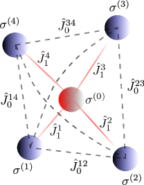
Figure 1: (Color online) Central spin model described by Eq. (5) with $M=4$. The solid lines represent the coupling between the central spin (qubit) and the spins of the bath, while the dashed lines represent the couplings between the spins of the bath.

The QDD sequence is made of an outer sequence of $\pi$-pulses about $\sigma_{x}$ and of an inner sequence of $\pi$-pulses about $\sigma_{z}$. The number of pulses for each sequence is $N_{x}$ and $N_{z}$, respectively, and the total number of pulses of the sequence is $N_{x}+N_{z}+N_{x}N_{z}$. The switching instants are given by

$$t^{x}_{j}=\tau\sin^{2}\left[\frac{j\pi}{2(N_{x}+1)}\right]$$ (6a)

$$t^{z}_{k,j}=t^{x}_{j}+(t^{x}_{j+1}-t^{x}_{j})\sin^{2}\left[\frac{k\pi}{2(N_{z}+1)}\right]$$ (6b)

for $j=\{1,..,N_{x}\}$ and $k=\{1,..,N_{z}\}$. We use the notation $t^{x}_{N_{x}+1}=\tau$.

We start with an initial density matrix of the total system of the form

$$\rho_{0}^{(\gamma)}=|\gamma\rangle\langle\gamma|\otimes\rho_{\text{B}},$$ (7)

with $\gamma=\{x,y,z\}$. The first factor in the tensor product refers to the Hilbert space of the qubit, the second to the Hilbert space of the bath. Furthermore, we introduce the notation

$$\rho_{0}^{(\gamma)}:=\rho_{\text{S}}^{(\gamma)}\otimes\rho_{\text{B}}.$$ (8)

For the low symmetry case we assume that the bath is initially in a pure product state

$$|\psi_{\text{B}}\rangle=\bigotimes_{i=1}^{M}|\gamma_{i}\rangle$$ (9)

so that $\rho_{\text{B}}=|\psi_{\text{B}}\rangle\langle\psi_{\text{B}}|$. For the high symmetry case we choose

$$\rho_{\text{B}}=\mathbbm{1}_{\text{B}}/D$$ (10)

where $D$ is the dimension of the Hilbert space of the bath so that $\text{Tr}_{\text{B}}\rho_{\text{B}}=1$.

The overall performance of the sequence is given by the norm distance Lidar et al. (2008)

$$d^{2} := \frac{1}{3}\sum_{\gamma\in\{x,y,z\}}d^{2}_{\gamma}$$ (11a)

$$d^{2}_{\gamma} := \text{Tr}_{\text{q}}\left[\Delta^{(\gamma)}(\tau)\right]^{2},$$ (11b)

with

$$\Delta^{(\gamma)}(\tau):=\text{Tr}_{\text{B}}\left(U_{\text{B}}\hat{P}\rho_{0}^{(\gamma)}\hat{P}^{\dagger}U_{\text{B}}^{\dagger}-U(\tau,0)\rho_{0}^{(\gamma)}U(\tau,0)^{\dagger}\right).$$ (12)

The norm distance measures the distance of the real evolution to the ideal one. The operator $\hat{P}$ is defined by

$$\hat{P}:=\underset{N_{x}+1}{\underbrace{\sigma_{z}^{N_{z}}\sigma_{x}\sigma_{z}^{N_{z}}\sigma_{x}...\sigma_{z}^{N_{z}}}}.$$ (13)

It incorporates the effects of the pulses. The operator $U(\tau,0)$ represents the evolution operator of the system (5)

$$U(\tau,0)={\cal T}\left\{e^{-i\int_{0}^{\tau}H(t)\text{d}t}\right\},$$ (14)

where ${\cal T}$ stands for the time-ordering and

$$U_{\text{B}}:=\mathbbm{1}\otimes e^{-i\tau H_{\text{B}}}$$ (15)

is the dynamics of the isolated bath. During the application of the sequence the sign in front of the coupling terms between the qubit and the bath perpendicular to the pulse direction changes every time a $\pi$ pulse is applied because $\sigma_{i}\sigma_{j}=-\sigma_{j}\sigma_{i}$ for $i\neq j$. Thus, in the toggling frame, the system Hamiltonian (5) can be written as a time dependent Hamiltonian

$$H(t)=H_{\text{B}}+\sum_{i=1}^{M}\sum_{j,k=1}^{3}f_{j}(t)\ \sigma^{(0)}_{j}\left(J_{1}^{i}\right)_{jk}\sigma_{k}^{(i)},$$ (16)

where the switching functions $f_{j}(t)$ are a piecewise constant functions with values $\pm 1$. By $\sigma_{k}^{(i)}$ we refer to the $k$ component of the vector $\vec{\sigma}^{(i)}$. Analogously, we refer by $\left(J_{1}^{i}\right)_{jk}$ to the $(j,k)$ element of the matrix $\hat{J}_{1}^{i}$.

Our simulations show that for $N_{x}\neq 0$, $N_{z}\neq 0$ and

$$\begin{array}[]{c}\text{for}\ N_{x}=N_{z}=N\rightarrow d\propto\tau^{N+1}+{\cal O}\left(\tau^{N+2}\right),\end{array}$$ (17b)

$$\begin{array}[]{c}\text{for}\ N_{x}>N_{z}\rightarrow d\propto\tau^{N_{z}+1}+{\cal O}\left(\tau^{N_{z}+2}\right),\end{array}$$ (17d)

$$\begin{array}[]{c}\text{for}\ N_{x}<N_{z}\rightarrow d\propto\tau^{N_{x}+1}+{\cal O}\left(\tau^{N_{x}+2}\right),\end{array}$$ (17f)

as shown in Tab. 2 and in Fig. 2. The data agree with the results of Ref. Quiroz and Lidar, 2011 for the overall error. For either $N_{x}=0$ or $N_{z}=0$ (UDD sequence) we find that $d$ scales as $\tau$, as expected for a Hamiltonian with general decoherence. On the other hand, if $N_{z}=0$ for example and $H_{\text{qB}}$ is a pure dephasing Hamiltonian, i.e., no couplings with $\sigma_{x}^{(0)}$ or with $\sigma_{y}^{(0)}$ occur in the Hamiltonian, the norm distance scales as $d_{\text{UDD}}\propto\tau^{N_{x}+1}$.

Here we present the results of a given random configuration of the entries of $\hat{J}_{0}^{ij}$ and $\hat{J}_{1}^{i}$. We also checked that the scaling is the same for other random configurations.

$N_{z}\setminus N_{x}$	0	1	2	3	4	5	6
0	1.00	1.00	1.00	1.00	1.00	1.00	1.00
1	1.00	2.01	2.00	2.01	2.01	2.01	2.00
2	1.00	2.01	2.97	3.01	3.01	3.01	3.02
3	1.00	2.00	2.99	4.01	4.07	4.09	4.09
4	1.00	2.00	3.00	4.01	4.99	4.98	5.05
5	1.00	1.95	3.02	3.95	5.01	5.98	6.05
6	1.00	1.98	3.01	3.94	5.00	5.84	6.95

Table 2: Low symmetry case: Scaling exponent $\zeta$ of the norm distance $d(\tau)$ with $\tau$, the total duration of the sequence. The reported numbers are determined from the slope of the curve $d$ vs. $\tau$ in a double logarithmic plot.

Different choices of the initial bath state $\rho_{\text{B}}$ of the form (9), i.e., varying the $|\gamma_{i}\rangle$, can affect the scaling of $d_{x}$, $d_{y}$ and of $d_{z}$, but not the overall scaling of $d$: If $d_{\gamma}\propto\tau^{A_{\gamma}}$ then the leading order of the norm distance scales as $d\propto\tau^{\min_{\gamma}\{A_{\gamma}\}}$. Hence the scaling exponent reads $\zeta=\min_{\gamma}\{A_{\gamma}\}$. This is what the analytic arguments require for QDD Wang and Liu (2011); Jiang and Imambekov (2011); W.-J-Kuo and Lidar (2011). Hence the analytic bounds on the exponents are sharp for the low symmetry case.

III Case 2: High Symmetry

We consider an SU(2) invariant isotropic central spin model with Heisenberg couplings. We choose a Hamiltonian of the form of Eq. (5) with $\hat{J}_{0}^{ij}=\alpha\lambda j_{0}^{ij}\mathbbm{1}$ and $\hat{J}_{1}^{i}=\lambda j_{1}^{i}\mathbbm{1}$, where $\alpha$ and $\lambda$ are two generic constants while $j_{0}^{ij}$ and $j_{1}^{i}$ are random numbers between $-1$ and $1$.

$N_{z}\setminus N_{x}$	0	1	2	3	4	5	6
0	1.99	2.00	2.00	2.00	2.00	2.00	2.00
1	2.00	3.99	3.95	4.00	3.98	4.00	4.00
2	2.00	4.00	5.99	6.13	6.00	5.99	5.99
3	2.00	3.99	5.99	7.98	7.97	8.01	8.01
4	2.00	4.00	5.99	7.99	9.97	9.92	9.94
5	2.00	4.00	5.99	7.99	9.97	11.93	11.94
6	2.00	4.00	6.00	7.97	9.95	12.01	13.95

Table 3: High symmetry case: Scaling exponent $\zeta$ of the norm distance with $\tau$ for an isotropic Hamiltonian with general decoherence and for an initial density matrix such as in Eq. (18). The scaling exponent are derived from a fit of the numerical curves for $d$ vs. $\tau$ in a double logarithmic plot.

If the bath at $t=0$ is described by the following density matrix

$$\rho_{\text{B}}\propto\mathbbm{1}_{\text{B}},$$ (18)

the suppression of the decoherence is enhanced by a factor 2. The simulation for QDD yields the scaling exponents reported in Tab. 3. We deduce the following rules: for $N_{x}\neq 0$, $N_{z}\neq 0$ and

$$\begin{array}[]{c}N_{x}=N_{z}=N\rightarrow d\propto\tau^{2(N+1)}+{\cal O}\left(\tau^{2N+3}\right),\end{array}$$ (19b)

$$\begin{array}[]{c}N_{x}>N_{z}\rightarrow d\propto\tau^{2(N_{z}+1)}+{\cal O}\left(\tau^{2N_{z}+3}\right),\end{array}$$ (19d)

$$\begin{array}[]{c}N_{x}<N_{z}\rightarrow d\propto\tau^{2(N_{x}+1)}+{\cal O}\left(\tau^{2N_{x}+3}\right),\end{array}$$ (19f)

If $N_{x}=0$ or $N_{z}=0$ the norm distance scales as $\tau^{2}$. A graphical representation of the data is provided in Fig. 2.

The state of Eq. (18) is a completely disordered state where no particular spin direction or state is singled out. Such a state can be referred to as an “infinite-temperature” state. This is not unusual in NMR experiments where already at room temperature one finds $\hbar\omega_{\text{L}}/k_{\text{B}}T\approx 10^{-5}$, where $\omega_{\text{L}}$ is the Larmor frequency of a spin and $k_{\text{B}}$ is the Boltzmann constant. This means that the thermal energy exceeds all internal energy scales by many orders of magnitude.

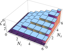
Figure 2: (Color online) The data of Tabs. 2 and 3 are graphically represented in panel (a) and in panel (b), respectively. The numbers are rounded to their first digit. Here we have introduced the notation here $d\propto\tau^{\zeta}$, where $\zeta$ stands for the scaling exponents.

Note that for $\rho_{\text{B}}\propto\mathbbm{1}_{\text{B}}$ the norm distance (11) coincides with the partial Frobenius norm distance Pasini et al. (2011); Lidar et al. (2008).

IV SU(2) invariance

The appearance of the factor 2 can be explained in terms of the different parity of $H_{\text{B}}$ and $H_{\text{qB}}$ under spin rotations. We write the Hamiltonian (5) in the form

$$H=\mathbbm{1}_{\text{S}}\otimes A_{0}+\sum_{\mu\in\{x,y,z\}}\sigma_{\mu}\otimes A_{\mu}.$$ (20)

In Eq. (20) the operators $A_{0}$ and $A_{\mu}$ act only on the bath while $\mathbbm{1}_{\text{S}}$ and $\sigma_{\mu}$ act only on the qubit. Since the identity operator and the Pauli matrices form a complete basis for all system operators the evolution operator can be expanded according to

$$U(\tau,0)=\mathbbm{1}_{\text{S}}\otimes B_{0}(\tau)+\sum_{\mu=x,y,z}\sigma_{\mu}\otimes B_{\mu}(\tau),$$ (21)

where $B_{0}(\tau)$ and $B_{\mu}(\tau)$ are non-trivial functions of the operators $A_{0}$ and $A_{\mu}$ and of the switching functions $f_{\mu}(t)$, see Eq. (31) in the Appendix and Ref. Uhrig and Lidar, 2010. For the sake of simplicity we will omit the time dependence of the operators $B_{0}$ and $B_{\mu}$ from now on. From the unitarity of $U(\tau,0)$ we conclude

$$\mathbbm{1}_{\text{B}}=B_{0}B_{0}^{\dagger}+\sum_{\mu\in\{x,y,z\}}B_{\mu}B_{\mu}^{\dagger}$$ (22a)

and

$$0=i\sum_{\mu,\nu\in\{x,y,z\}}\epsilon_{\mu\nu\kappa}B_{\mu}B_{\nu}^{\dagger}+\left(B_{0}B_{\kappa}^{\dagger}+\text{h.c.}\right)$$ (22b)

for fixed $\kappa\in\{x,y,z\}$ and $\epsilon_{\mu\nu\kappa}$ being the Levi-Civita symbol. In (22b) we omitted the non-singular factor proportional to Pauli matrices because the vanishing must be ensured by the bath operators. In the Heisenberg picture the density matrix $\rho_{0}^{(\gamma)}$ (7) evolves according to

$$\rho_{0}^{(\gamma)}(\tau) = U(\tau,0)\rho_{0}^{(\gamma)}U(\tau,0)^{\dagger}$$ (23)

$$= U(\tau,0)\left(\rho_{\text{S}}^{(\gamma)}\otimes\rho_{\text{B}}\right)U(\tau,0)^{\dagger}.$$ (24)

We trace out the bath and use the unitarity of $U(\tau,0)$ (22) to obtain

$$\text{Tr}_{\text{B}}\ \rho_{0}^{(\gamma)}(\tau)=T_{1}^{(\gamma)}+T_{2}^{(\gamma)}+T_{3}^{(\gamma)}+T_{4}^{(\gamma)}$$ (25)

with

$$T_{1}^{(\gamma)}:= \rho_{\text{S}}^{(\gamma)}\text{Tr}_{\text{B}}\rho_{\text{B}}+\sum_{\mu\in\{x,y,z\}}(c_{\mu,\mu}^{(\gamma)}-\rho_{\text{S}}^{(\gamma)})\ b_{\mu,\mu},$$ (26a)

$$T_{2}^{(\gamma)}:= \sum_{\mu,\nu\in\{x,y,z\},\mu\neq\nu}c_{\mu,\nu}^{(\gamma)}\ b_{\mu,\nu},$$ (26b)

$$T_{3}^{(\gamma)}:= \sum_{\mu\in\{x,y,z\}}d_{\mu}^{(\gamma)}b_{\mu},$$ (26c)

$$T_{4}^{(\gamma)}:= -i\sum_{\mu,\nu,\kappa\in\{x,y,z\}}\epsilon_{\mu\nu\kappa}\ \rho_{\text{S}}^{(\gamma)}\sigma_{\kappa}\ b_{\nu,\mu}.$$ (26d)

The coefficients

$$b_{\mu,\nu} := \text{Tr}_{\text{B}}[B_{\mu}\rho_{\text{B}}B_{\nu}^{\dagger}]$$ (27a)

$$b_{\mu} := \text{Tr}_{\text{B}}\left[B_{0}\rho_{\text{B}}B_{\mu}^{\dagger}\right]$$ (27b)

depend only on the bath operators while $c_{\mu,\nu}^{(\gamma)}:=\sigma_{\mu}\rho_{\text{S}}^{(\gamma)}\sigma_{\nu}$ and $d_{\mu}^{(\gamma)}:=\sigma_{\mu}\rho_{\text{S}}^{(\gamma)}-\rho_{\text{S}}^{(\gamma)}\sigma_{\mu}$ are functions of the qubit operators only. Note that for a pure dephasing model Uhrig and Lidar (2010) the terms $T_{2}^{(\gamma)}$ and $T_{4}^{(\gamma)}$ do not appear.

We consider a global operator $\hat{P}_{\nu}$ that rotates all the spins of our system around the $\nu=x$, $y$, or $z$ axis by the angle $\pi$. Here we are interested in the SU(2) invariant Hamiltonian such as the one discussed in Sec. III. Then we have

$$\hat{P}_{\nu}B_{0}\hat{P}_{\nu}^{\dagger}=B_{0}\quad\hat{P}_{\nu}B_{\nu}\hat{P}_{\nu}^{\dagger}=B_{\nu}\ ,$$ (28a)

$$\hat{P}_{\nu}B_{\mu}\hat{P}_{\nu}^{\dagger}=-B_{\mu}\quad\text{for}\ \nu\neq\mu$$ (28b)

and therefore

$$b_{\mu} = \text{Tr}_{\text{B}}\left[B_{0}\rho_{\text{B}}B_{\mu}^{\dagger}\right]$$ (29a)

$$= \text{Tr}_{\text{B}}\left[\hat{P}_{\nu}B_{0}\hat{P}_{\nu}^{\dagger}\ \hat{P}_{\nu}\rho_{\text{B}}\hat{P}_{\nu}^{\dagger}\ \hat{P}_{\nu}B_{\mu}^{\dagger}\hat{P}_{\nu}^{\dagger}\right]$$ (29b)

$$= -\text{Tr}_{\text{B}}\left[B_{0}\ \hat{P}_{\nu}\rho_{\text{B}}\hat{P}_{\nu}^{\dagger}\ B_{\mu}^{\dagger}\right]$$ (29c)

for $\mu\neq\nu$. Thus, if $\rho_{\text{B}}$ is invariant under rotation $\hat{P}_{\nu}$, which is the case for $\rho_{\text{B}}\propto\mathbbm{1}_{\text{B}}$, we can conclude from (29c) that $b_{\mu}=0$ for $\mu\in\{x,y,z\}$. In fact, the analogous argument also implies $b_{\mu,\nu}=0$ for $\mu\neq\nu$, though we will not use this fact here. The condition $\mu\neq\nu$ is needed to ensure that we can flip the sign of the two factor $B_{\mu}$ and $B_{\nu}^{\dagger}$ separately.

If the coefficients $b_{\mu}$ vanish only the terms proportional to $b_{\mu,\nu}$ remain in Eq. (25). We know from the analytic properties of the QDD sequence that the operators $B_{\mu}$ with $\mu\in\{x,y,z\}$ all scale at least with $\tau^{N_{\textrm{min}}+1}$ where $N_{\textrm{min}}:=\min(N_{x},N_{z})$ Wang and Liu (2011); Jiang and Imambekov (2011); W.-J-Kuo and Lidar (2011) supported by numerical results in Ref. Quiroz and Lidar, 2011 and in the present work. Hence the coefficients $b_{\mu}$ scale with $\tau^{N_{\textrm{min}}+1}$ and the coefficients $b_{\mu,\nu}$ with $\tau^{2N_{\textrm{min}}+2}$. Hence the vanishing of the $b_{\mu}$ terms in Eq. (25) automatically reduce the decoherence by doubling the exponent in the scaling $d\propto\tau^{N_{\textrm{min}}+1}\to\tau^{2N_{\textrm{min}}+2}$ with the total duration $\tau$ of the sequence.

Note that for a model of pure dephasing, e.g., only $\sigma_{z}^{(0)}$ appears in (5b), we do not need the symmetry with respect to two operators $\hat{P}_{\mu}$. It is sufficient to have either $\hat{P}_{x}$ or $\hat{P}_{y}$ which invert $\sigma_{z}$ so that we can conclude that $b_{z}$ vanishes in order to know that the scaling exponent doubles. This was already seen in the numerical data presented and analyzed in Ref. Pasini et al., 2011.

V Case 3: Mixed Symmetry

$N_{z}\setminus N_{x}$	0	1	2	3	4	5	6
0	0.99	1.00	1.00	1.00	1.00	1.00	1.00
1	1.00	2.00	2.00	2.00	2.00	2.00	2.00
2	1.00	1.99	3.01	3.00	3.00	3.00	3.00
3	1.00	2.00	3.00	4.00	4.00	4.00	4.00
4	1.00	2.01	3.00	4.02	5.00	5.00	5.01
5	1.00	2.00	3.00	4.00	5.02	6.00	6.00
6	1.00	2.00	3.00	3.98	5.00	6.00	6.99

$N_{z}\setminus N_{x}$	0	1	2	3	4	5	6
0	1.98	2.00	2.00	2.00	2.00	2.00	2.00
1	2.00	2.00	2.00	2.00	2.00	2.00	2.00
2	2.00	3.99	6.00	5.75	5.99	5.99	5.99
3	2.00	4.00	5.80	4.00	4.00	4.00	4.00
4	2.00	4.00	6.00	7.96	9.96	10.27	10.30
5	2.00	3.97	5.97	7.97	9.85	6.00	6.00
6	2.00	4.00	5.99	7.99	9.95	11.93	13.92

Table 4: Mixed cases: In Table (a) the Hamiltonian is SU(2) invariant while the bath is initially prepared in a product state. In Table (b) the Hamiltonian is asymmetric of the form in Eq. (5), the entries of $\hat{J}_{0}^{ij}$ and $\hat{J}_{1}^{i}$ are all randomly chosen, and $\rho_{\text{B}}\propto\mathbbm{1}_{\text{B}}$.

Here we analyze the off-diagonal cases of Tab. 4. They are characterized either by a SU(2) invariant Hamiltonian and a low-symmetry bath state or by a low-symmetry Hamiltonian with a high-symmetry initial bath state $\propto\mathbbm{1}_{\text{B}}$. Because the Hamiltonian and the density matrix have a different degree of symmetry the analytical argument of Eq. (29a) for $b_{\mu}$ does not hold anymore.

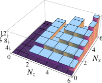
Figure 3: (Color online) The data of 4 (b) is graphically represented. The numbers are rounded to their first digit. The notation $\zeta$ refers to the scaling exponents of the norm distance $d\propto\tau^{\zeta}$.

The numerically found scaling exponents are reported in Tabs. 4 and depicted in Fig. 3. The coupling constants used to derive the scaling exponents of this Table are the same as those used for the simulation of the SU(2) invariant Hamiltonian or the ones used for the asymmetric Hamiltonians used in Secs. II and III.

If the Hamiltonian is SU(2) symmetric and the bath is initially prepared in a product state the scaling exponents look the same as those of Tab. 2. If the Hamiltonian is asymmetric and $\rho_{\text{B}}\propto\mathbbm{1}_{\text{B}}$ we find for $N_{x}=N_{z}=N$ that the scaling exponent is $N+1$ for $N$ odd and $2(N+1)$ for $N$ even. For $N_{x}>N_{z}$ the exponent is either $N_{z}+1$ if $N_{z}$ is odd or $2(N_{z}+1)$ if $N_{z}$ is even while for $N_{x}<N_{z}$ we find that $d$ scales as $2(N_{x}+1)$. We cannot provide any explanations for this alternating behavior of the scaling exponents and for the reason why, for $N_{x}>N_{z}$, it depends only on the number of pulses of the inner sequence. This is still an open question for future investigation.

Furthermore, it is worth mentioning that peculiar choices of the couplings imply non-generic behavior. If the couplings $j_{1}^{i}$ is the same for all $i$ the QDD sequence behaves like a UDD sequence with $N_{z}$ pulses for $N_{x}$ odd, as if the qubit were subject only to pure dephasing: Either $A_{x}\neq 0$ or $A_{y}\neq 0$ in Eq. 20. It is not clear why the QDD behaves like a UDD sequence in this case. A possible explanation is that the product state we take as initial state of the bath is not the most general one. It is not entangled. In the Appendix we analyze the first three cumulants of the evolution operator for the case $N_{x}=1$. We find that they contain only one qubit operator, either $\sigma_{x}$ or $\sigma_{y}$, and that the dephasing term proportional to $\sigma_{z}$ is always zero. For $N_{x}$ even we recover the results of Table 2.

VI Conclusions

We investigated the influence of the state of the bath in suppressing general decoherence by means of a QDD sequence. The performance of the sequence is measured by the norm distance $d$ which is essentially the norm of the remaining decoherence. Thus the performance is quantified by the scaling of $d$ with $\tau$, the total duration of the sequence. Recent papers Wang and Liu (2011); Jiang and Imambekov (2011); Quiroz and Lidar (2011); W.-J-Kuo and Lidar (2011) proved the properties of QDD and clarified the dependence of the scaling on the number of pulses $N_{x}$ and $N_{z}$: The overall scaling of QDD is given by $\zeta:=\min\{N_{x},N_{z}\}+1$ independent of the details of the environment, i.e., $d\propto\tau^{\zeta}$. In this sense QDD is a universal sequence for general decoherence such as UDD is a universal sequence for pure dephasing.

In the present work, we have shown that the actual performance of QDD can be even better than expected on the basis of the general mathematical arguments. This improvement occurs if the Hamiltonian and the bath state are highly symmetric, for instance, if the Hamiltonian is spin isotropic and the bath is prepared initially in a completely disordered state. Then we found both numerically and analytically that the exponent of the scaling with $\tau$ acquires an additional factor of 2: $d\propto\tau^{2\zeta}$. The same was already observed for the UDD sequence applied to pure dephasing in Ref. Pasini et al., 2011.

We emphasize that this result is by no means at odds with the proofs of universality Wang and Liu (2011); Jiang and Imambekov (2011); W.-J-Kuo and Lidar (2011). The general proofs refer to the worst case for decoherence. They determine whether a certain operator (Pauli matrix) for the qubit occurs or not irrespective of the bath operator to which it is multiplied. The underlying idea is that for any non-vanishing bath operator there is a bath state such that the qubit state is influenced in a non-trivial way. Hence decoherence occurs.

But for certain choices of the bath state even a non-vanishing bath operator may have a vanishing effect on the quantum bit if its partial bath trace vanishes. Then no decoherence is induced by this particular term. This is the effect which enhances the performance of the QDD sequence for highly symmetric situations. We summarize that $\min\{N_{x},N_{z}\}+1$ is a lower bound for $\zeta$.

We stress that the found phenomenon is relevant for realistic situations. Complete or partial spin symmetry in the Hamiltonian is a standard feature. A completely disordered bath state is also an excellent starting point in the description of baths of nuclear spins. Their mutual interaction is so small in energy that even room temperature suffices to disorder the nuclear spins completely.

In general, we conclude that the more asymmetric the bath Hamiltonian, its coupling to the qubit, and in particular its initial state are, the lower the exponent $\zeta$ is of the leading non-vanishing power in the total duration $\tau$ of the sequence inducing decoherence. The same is true of UDD sequences for pure dephasing. So far, we focussed on spin baths which allow for completely disordered, infinite temperature states. It is an interesting question for future research whether a similar phenomenon can occur in other baths such as bosonic ones.

Experimental research is also called for. To our knowledge, there exist studies on the influence of the initial state, see for instance Ref. Álvarez et al., 2010, but they focus on the initial state of the system. Discussions of the influence of the initial state of the bath, which was our focus here, are scarce Li et al. (2008). Moreover, it must be distinguished between studies of iterated cycles of sequences with exponential decay rates Ajoy et al. (2011) and studies of a single sequence displaying decoherence with a particular power law Uhrig (2007); Lee et al. (2008); Uhrig (2008); Yang and Liu (2008); West et al. (2010); Wang and Liu (2011); Jiang and Imambekov (2011); W.-J-Kuo and Lidar (2011).

Of course, it is difficult to measure the exponents directly. But we suggest to demonstrate experimentally that the performance of a QDD or a UDD sequence is lowered if the symmetry of either the Hamiltonian or of the initial bath state is lowered. This would already be a smoking gun evidence for the essence of the present theoretical finding.

Appendix A Magnus expansion of the evolution operator

In general, it is complicated to find a universal argument that explains the scaling of QDD if the symmetry of the system is not well defined. The reason why some exponents deviate from the analytically predicted value depends on the possible vanishing of some terms in the Magnus expansion Haeberlen (1976); Magnus (1954) of the evolution operator. The form of such terms strongly depends on the form of the Hamiltonian and of the symmetry of the bath state.

If no general conclusions can be drawn on the parity of these terms and of the density matrix under a rotation $\hat{P}_{\mu}$, one way to proceed is to calculate the cumulants of the expansion explicitly and to analyze which terms determine the power law of $d$ with $\tau$. Here we provide an analysis of the first cumulants of the Magnus expansion for $N_{x}$ odd for the data of Tab. 4(a).

For a generic instant $t\in[0,\tau]$ we write the Hamiltonian (5) as

$$H(t)=H_{\text{B}}+\sum_{\mu=x,y,z}\sigma_{\mu}f_{\mu}(t)A_{\mu}.$$ (30)

The switching functions $f_{\mu}(t)$ are the effect of the stroboscopic pulsing of the qubit. They are piecewise constant functions with values $\pm 1$

$$f_{z}(t)=(-1)^{j}\quad\text{for}\quad t\in(t^{x}_{j},t^{x}_{j+1}],$$ (31a)

$$f_{y}(t)=(-1)^{k}\quad\text{for}\quad t\in(t^{z}_{j,k},t^{x}_{j+1,k}],$$ (31b)

with $$f_{y}(0)=1 f_{y}(\tau)=-1$$ and , and

$$f_{x}(t)=f_{z}(t)f_{y}(t).$$ (31c)

The evolution operator can be written in terms of the cumulants $\bar{H}^{(n)}$ as

$$U(\tau,0) = \exp\{-i\tau\sum_{n=1}^{\infty}\bar{H}^{(n)}\}$$ (32)

with $\tau\bar{H}^{(n)}\propto\tau^{n}$. The first and the second cumulants are defined Haeberlen (1976) as $\tau\bar{H}^{(1)}=\int_{0}^{\tau}H(t)\text{d}t$, $\tau\bar{H}^{(2)}=-\frac{i}{2\tau}\int_{0}^{\tau}\text{d}t_{1}\int_{0}^{t_{1}}\text{d}t_{2}\left[H(t_{1}),H(t_{2})\right]$. From Eqs. (31) it is straightforward to verify that $\int_{0}^{\tau}\text{d}tf_{\mu}(t)=0$ for $\mu=x$, $y$ or $z$ and for $N_{z}=N_{x}=1$. The first cumulant is proportional to the bath Hamiltonian

$$\tau\bar{H}^{(1)}=\tau H_{\text{B}}.$$ (33)

For the second cumulant one finds

$$2i\tau\bar{H}^{(2)}=\sum_{\mu=x,y,z}\sigma_{\mu}I_{2}^{\mu}\left[H_{\text{B}},A_{\mu}\right]$$ (34)

$$+\sum_{\mu,\nu=x,y,z}I_{2}^{\mu,\nu}\left[\sigma_{\mu}A_{\mu},\sigma_{\nu}A_{\nu}\right],$$ (35)

with the integrals

$$I_{2}^{\mu}:=\int_{0}^{\tau}\text{d}t_{1}\int_{0}^{t_{1}}\text{d}t_{2}\left(f_{\mu}(t_{2})-f_{\mu}(t_{1})\right)$$ (36a)

and

$$I_{2}^{\mu,\nu}:=\int_{0}^{\tau}\text{d}t_{1}\int_{0}^{t_{1}}\text{d}t_{2}f_{\mu}(t_{2})f_{\nu}(t_{1}).$$ (36b)

The integrals (36a) and (36b) can be easily evaluated, we report below only those that are different from zero. For $N_{z}=N_{x}=1$ one finds

$$I_{2}^{y}=\frac{\tau^{2}}{4},\quad I_{2}^{z}=\frac{\tau^{2}}{2},\quad I_{2}^{x,z}=-I_{2}^{z,x}=-\frac{\tau^{2}}{4}.$$ (37)

The second cumulant then becomes

$$2i\tau\bar{H}^{(2)} =\frac{\tau^{2}}{4}\sigma_{y}\left[H_{\text{B}},A_{y}\right]+\frac{\tau^{2}}{2}\sigma_{z}\left[H_{\text{B}},A_{z}\right]$$

$$+i\frac{\tau^{2}}{2}\sigma_{y}\left[A_{x},A_{z}\right]_{+},$$ (38)

where the notation $[\ ,\ ]_{+}$ stands for an anticommutator. It is interesting to notice that $\bar{H}^{(2)}$ does not contain any terms proportional to $\sigma_{x}$.

If the Hamiltonian is SU(2) invariant and the coupling constants $\hat{J}_{0}^{ij}$ and $\hat{J}_{1}^{i}$ are equal and independent of the indexes $i$ and $j$ ($\hat{J}_{0}^{ij}=\alpha\lambda$ and $\hat{J}_{1}^{i}=\lambda$) the commutators in Eq. (A) vanish because the Pauli matrices anticommute. This is true for a central spin model.

On the other hand, if $A_{\mu}\equiv\sigma_{\mu}^{(1)}$ (e.g. for a spin chain) the commutators in Eq. (A) are different from zero. The anticommutator becomes $\left[A_{x},A_{z}\right]_{+}=2i\sum_{i,j}(\hat{J}_{1})_{xx}(\hat{J}_{1})_{zz}(1-\delta_{ij})\sigma_{x}^{(i)}\sigma_{z}^{(j)}$ which implies that it vanishes for a spin chain because the qubit is coupled to a single site only, i.e., $i=j$ holds.

As usual we are interested in the difference between the evolved density matrix $\rho_{0}^{(\gamma)}(\tau)=U(\tau,0)\rho_{0}^{(\gamma)}U(\tau,0)^{\dagger}$ and the initial one. We find

$$\text{Tr}_{\text{B}}\left\{\rho_{0}^{(\gamma)}(\tau)-\rho_{0}^{(\gamma)}\right\}=\frac{\tau^{2}}{4}[\sigma_{y},\rho_{\text{S}}^{(\gamma)}]\ \text{Tr}_{\text{B}}\left\{\rho_{\text{B}}\left[A_{x},A_{z}\right]_{+}\right\}$$

$$\qquad+\frac{\tau^{4}}{16}\ c_{yy}^{(\gamma)}\ \text{Tr}_{\text{B}}\left\{\left[A_{x},A_{z}\right]_{+}\rho_{\text{B}}\left[A_{x},A_{z}\right]_{+}\right\}$$ (39)

where the hermitecity $A_{\mu}^{\dagger}=A_{\mu}$ was used. In writing Eq. (A) we neglected the contributions coming from the first cumulant because they do not alter the qubit-operator content of the norm distance.

If $\rho_{\text{B}}\propto\mathbbm{1}_{\text{B}}$ the terms with the trace over the bath vanish for a SU(2) invariant Hamiltonian (see Sect. III) while they are finite for an asymmetric model such as the one in Eq. (5) in Sect. II.

In order to understand why the distance norm scales with exponents $N_{z}+1$ for $N_{x}=1$ (and in general for $N_{x}$ odd) in Tab. 4(a), some knowledge on the third cumulant $\bar{H}^{(3)}$ is required. This cumulant is defined Haeberlen (1976) as

$$-6\tau\bar{H}^{(3)}=\int_{0}^{\tau}\text{d}t_{1}\int_{0}^{t_{1}}\text{d}t_{2}\int_{0}^{t_{2}}\text{d}t_{3}\ \times$$

$$\left\{[H(t_{3}),[H(t_{2}),H(t_{1})]]+[H(t_{1}),[H(t_{2}),H(t_{3})]]\right\}.$$ (40)

The commutators $[H(t_{2}),H(t_{1})]$ and $[H(t_{2}),H(t_{3})]$ have the same operator content as $\bar{H}^{(2)}$, but differ in their prefactors and in their time dependence. One can verify that $[H_{\text{B}},\bar{H}^{(2)}]=0$ if the bath Hamiltonian is SU(2) invariant due to the anticommutation of the Pauli matrices. For the same reason one finds that

$$\left[\sum_{\mu}\sigma_{\mu}A_{\mu},\bar{H}^{(2)}\right]\propto\sum_{\mu,\nu}\epsilon_{\mu,y,\nu}\ \sigma_{\nu}\otimes\sigma_{x}^{(i)}\sigma_{y}^{(j)}\sigma_{\mu}^{(k)},$$ (41)

where $i\neq j\neq k$. Equation (41) only provides the operator contents of Eq. (A). In order to eliminate the time dependence one must substitute Eq. (41) into Eq. (A) and integrate over $t_{1}$, $t_{2}$ and $t_{3}$. Each operator $A_{\mu}$ brings a switching function $f_{\mu}(t)$ with it, such that the integration in (A) yields the coefficients

$$I_{3}^{\alpha,\beta,\gamma}=\int_{0}^{\tau}\text{d}t_{1}\int_{0}^{t_{1}}\text{d}t_{2}\int_{0}^{t_{2}}\text{d}t_{3}f_{\alpha}(t_{1})f_{\beta}(t_{2})f_{\gamma}(t_{3}).$$ (42)

The indices $\alpha$, $\beta$ and $\gamma$ can be equal to $x$, $y$, and $z$. We have checked numerically that for $N_{x}=1$ and $N_{z}=2$ the only non-zero contributions are given by $I_{3}^{x,z,z}$, $I_{3}^{z,x,z}$ and $I_{3}^{z,z,x}$ corresponding to the qubit operator $\sigma_{x}$. Thus the third cumulant $\bar{H}^{(3)}$ is a term of pure dephasing that can be suppressed by means of a $Z$ sequence of $\pi$ pulses. From the numerical results we expect that the same argument holds in general for higher cumulants and for $N_{x}$ odd.

We also checked our results for a spin chain. We find the same results as for a central spin model in the cases of low symmetry, high symmetry and in the case of an asymmetric Hamiltonian with $\rho_{\text{B}}\propto\mathbbm{1}_{\text{B}}$. Discrepancies are found for the SU(2) invariant Hamiltonian in combination with the product state $|\psi_{\text{B}}\rangle$ (9). A possible explanation is provided by the commutators in Eq. (A) that do not vanish for a spin chain with $A_{\mu}=\sigma_{\mu}^{(1)}$. Hence the precise topology of the model matters for the case of mixed degree of symmetry.

References

- Viola and Lloyd (1998) L. Viola and S. Lloyd, Phys. Rev. A 58, 2733 (1998).
- Hahn (1950) E. L. Hahn, Phys. Rev. 80, 580 (1950).
- Carr and Purcell (1954) H. Y. Carr and E. M. Purcell, Phys. Rev. 94, 630 (1954).
- Meiboom and Gill (1958) S. Meiboom and D. Gill, Rev. Sci. Inst. 29, 688 (1958).
- Uhrig (2007) G. S. Uhrig, Phys. Rev. Lett. 98, 100504 (2007).
- Yang and Liu (2008) W. Yang and R.-B. Liu, Phys. Rev. Lett. 101, 180403 (2008).
- Uhrig (2008) G. S. Uhrig, New J. Phys. 10, 083024 (2008).
- Uhrig (2009) G. S. Uhrig, Phys. Rev. Lett. 102, 120502 (2009).
- Biercuk et al. (2009) M. J. Biercuk, H. Uys, A. P. VanDevender, N. Shiga, W. M. Itano, and J. J. Bollinger, Nature 458, 996 (2009).
- Uys et al. (2009) H. Uys, M. J. Biercuk, and J. J. Bollinger, Phys. Rev. Lett. 103, 040501 (2009).
- Khodjasteh et al. (2011) K. Khodjasteh, T. Erdélyi, and L. Viola, Phys. Rev. A 83, 020305(R) (2011).
- Khodjasteh and Lidar (2005) K. Khodjasteh and D. A. Lidar, Phys. Rev. Lett. 95, 180501 (2005).
- West et al. (2010) J. R. West, B. H. Fong, and D. A. Lidar, Phys. Rev. Lett. 104, 130501 (2010).
- Pasini and Uhrig (2008) S. Pasini and G. S. Uhrig, J. Phys. A: Math. Theo. 41, 312005 (2008).
- Wang and Liu (2011) Z.-Y. Wang and R.-B. Liu, Phys. Rev. A 83, 022306 (2011).
- Jiang and Imambekov (2011) L. Jiang and A. Imambekov, p. 1104.5021 (2011).
- W.-J-Kuo and Lidar (2011) W.-J-Kuo and D. A. Lidar, p. 1106.2151 (2011).
- Quiroz and Lidar (2011) G. Quiroz and D. A. Lidar, p. 1105.4303 (2011).
- Cywiński et al. (2008) L. Cywiński, R. M. Lutchyn, C. P. Nave, and S. Das Sarma, Phys. Rev. B 77, 174509 (2008).
- Pasini and Uhrig (2010) S. Pasini and G. S. Uhrig, Phys. Rev. A 81, 012309 (2010).
- Du et al. (2009) J. Du, X. Rong, N. Zhao, Y. Wang, J. Yang, and R. B. Liu, Nature 461, 1265 (2009).
- Ajoy et al. (2011) A. Ajoy, G. A. Álvarez, and D. Suter, Phys. Rev. A 83, 032303 (2011).
- Jenista et al. (2009) E. R. Jenista, A. M. Stokes, R. T. Branca, and W. S. Warren, J. Chem. Phys. 131, 204510 (2009).
- Schliemann et al. (2003) J. Schliemann, A. Khaetskii, and D. Loss, J. Phys.: Condens. Matter 15, R1809 (2003).
- Bortz and Stolze (2007a) M. Bortz and J. Stolze, J. Stat. Mech. p. P06018 (2007a).
- Bortz and Stolze (2007b) M. Bortz and J. Stolze, Phys. Rev. B 76, 014304 (2007b).
- Witzel and Das Sarma (2008) W. M. Witzel and S. Das Sarma, Phys. Rev. B 77, 165319 (2008).
- Lee et al. (2008) B. Lee, W. M. Witzel, and S. Das Sarma, Phys. Rev. Lett. 100, 160505 (2008).
- Pasini et al. (2011) S. Pasini, P. Karbach, and G. S. Uhrig, Europhys. Lett. p. 1009.2638 (2011).
- Lidar et al. (2008) D. Lidar, P. Zanardi, and K. Khodjasteh, Phys. Rev. A 78, 012308 (2008).
- Uhrig and Lidar (2010) G. S. Uhrig and D. A. Lidar, Phys. Rev. A 82, 012301 (2010).
- Álvarez et al. (2010) G. A. Álvarez, A. Ajoy, X. Peng, and D. Suter, Phys. Rev. A 82, 042306 (2010).
- Li et al. (2008) D. Li, Y. Dong, R. G. Ramos, J. D. Murray, K. MacLean, A. E. Dementyev, and S. E. Barrett, Phys. Rev. B 77, 214306 (2008).
- Haeberlen (1976) U. Haeberlen, High Resolution NMR in Solids: Selective Averaging (Academic Press, New York, 1976).
- Magnus (1954) W. Magnus, Comm. Pure Appl. Math. 7, 649 (1954).