Interplay between quantum interference and Kondo effects in non-equilibrium transport through nanoscopic systems

Abstract

We calculate the finite temperature and non-equilibrium electric current through systems described generically at low energy by a singlet and two spin doublets for $N$ and $N\pm 1$ electrons respectively, coupled asymmetrically to two conducting leads, which allows for destructive interference in the conductance. The model is suitable for studying transport in a great variety of systems such us aromatic molecules, different geometries of quantum dots and rings with applied magnetic flux. As a consequence of the interplay between interference and Kondo effect, we find changes by several orders of magnitude in the values of the conductance and its temperature dependence as the doublet level splitting is changed by some external parameter. The differential conductance at finite bias is negative for some parameters.

Transport properties of single molecules are being extensively studied due to their potential use as active components of new electronic devices. Experimental results show an increased conductance at low temperatures due to the usual spin-1/2 or spin-1 Kondo effect and quantum phase transitions were induced changing externally controlled parameters park ; lian ; roch ; parks ; serge . Measurements through single $\pi$-conjugated molecules park ; venk ; dani ; dado stimulated further theoretical work. In particular, the possibility of controlling molecular electronics using quantum interference effects in annulene molecules has been recently proposed carda ; ke ; bege ; mole . The conductance depends on which sites of the molecule are coupled to the leads and on interference phenomena related to the symmetry of the system. For certain conditions it can be totally suppressed and restored again by symmetry-breaking perturbations mole .

Interference phenomena are also well known in rings threaded by a magnetic flux. While sizable fluxes are at present impossible to apply to small annulene molecules due to their small area, Aharonov-Bohm oscillations were observed in systems involving two quantum dots (QDs).hata Systems of three waugh ; gaud ; rogge , and more kouw QDs have been assembled to study the effects of interdot hopping on the Kondo effect, and other physical properties driven by strong correlations. It has been predicted that the transmittance integrated over a finite energy window jagla ; frie ; hall or the conductance through a ring of strongly correlated one-dimensional systems hall ; rinc display dips as a function of the applied magnetic flux at fractional values of the flux quantum, due to spin-charge separation. While the energy integration mimics a finite bias voltage $V$ or temperature $T$ applied to the system, the calculations were actually performed at $V=T=0$. Moreover, as in calculations of transport through molecules which included the effect of correlations bege ; mole ; hett , the leads were included perturbatively, missing the Kondo regime, for which the conductance is usually the highest soc . The Kondo effect was also missed in previous studies of interference effects at equilibrium ($V=0$) for three dots at $T>T_{K}$ kuz , where $T_{K}$ is the Kondo temperature of the system, and in the spinless case meden . Experimentally, the crossing of levels and the ensuing destructive interference has been induced applying magnetic field to a system with large, level-dependent $g$ factors nils .

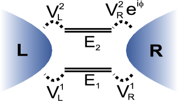
Figure 1: Scheme of the relevant matrix elements at low energies.

An analysis of the current through finite rings shows that interference phenomena take place when two levels become degenerate rinc . In the case of annulene molecules these states correspond to two doublets with total wave vectors $\pm K$, degenerate due to reflection symmetry (in absence of an external flux) bege ; mole ; rinc . For the infinite-$U$ Hubbard model, the interfering states differ in the spin quantum numbers rinc .

In this work we study the non-equilibrium transport in a generalized Anderson model, whose localized part consists of a singlet with even $N$ electrons and two doublets with $N\pm 1$ electrons (see Fig. 1). The model describes the low-energy physics and interference phenomena of a wide range of physical systems, such as those mentioned above. This calculation is a substantial improvement to previous results on conductance through interacting systems with interfering effects, mole ; jagla ; frie ; hall ; rinc since it introduces the relevant Kondo regime neglected in those studies as well as finite temperature and non-equilibrium effects at finite gate voltages.

Due to its reliability, for this study we use the non-crossing approximation (NCA) nca ; nca2 . For the case of one doublet, comparison of NCA with numerical renormalization group (NRG) results compa , shows that the NCA describes accurately the Kondo physics and in addition, allows us to reach finite bias voltages and temperatures. The leading behavior of the differential conductance with voltage is the correct one and $G(T)/G(0)$ practically coincides with the NRG result over several decades of temperature roura . The results should improve with increasing degeneracy (small or zero level splitting in our case) and in fact experimental observations near quantum phase transitions were well reproduced by the NCA serge ; nca2 . We calculate the effects of interference on non-equilibrium conductance in a regime of gate voltages for which the doublets are favored, leading to Kondo effect and high values of the conductance. In this approximation we asume that other higher-lying levels are negligible for the range of parameters considered.

The effective Hamiltonian is

$$H = E_{s}|0\rangle\langle 0|+\sum_{i\sigma}E_{i}|i\sigma\rangle\langle i\sigma|+\sum_{\nu k\sigma}\epsilon_{\nu k}c_{\nu k\sigma}^{\dagger}c_{\nu k\sigma}$$ (1)

$$+\sum_{i\nu k\sigma}(V_{\nu}^{i}|i\sigma\rangle\langle 0|c_{\nu k\sigma}+\mathrm{H.c}.),$$

where the singlet $|0\rangle$ and the two doublets $|i\sigma\rangle$ ($i=1,2$; $\sigma=\uparrow$ or $\downarrow$) denote the localized states, $c_{\nu k\sigma}^{\dagger}$ create conduction states in the left ($\nu=L$) or right ($\nu=R$) lead, and $V_{\nu}^{i}$ describe the hopping elements between the leads and both doublets, assumed independent of $k$. By a gauge transformation, three of the four $V_{\nu}^{i}$ can be made real and positive. If the system is a ring with the leads $\nu$ connected at sites $j_{\nu}$, the remaining effective hopping can be chosen as $V_{R}^{2}=|V_{R}^{2}|e^{-i\phi}$, where $\phi=(j_{R}-j_{L})(K_{2}-K_{1})$, and $K_{i}$ is the wave vector of $|i\sigma\rangle$ rinc . The magnitude of the hoppings is given by $|V_{\nu}^{i}|=|t_{\nu}\langle i\sigma|d_{j_{\nu}\sigma}^{\dagger}|0\rangle|$, where $t_{\nu}$ is the hopping between site $j_{\nu}$ and the lead $\nu$, and $d_{j\sigma}^{\dagger}$ creates an electron (or a hole depending on the sign of the gate voltage) at site $j$ ihm . If both doublets are related by a symmetry operation in the absence of an applied magnetic flux (for example reflection symmetry), then $|V_{\nu}^{1}|=|V_{\nu}^{2}|$. If, in addition, $\phi=\pi$ and $E_{2}=E_{1}$, the state $|L\sigma\rangle=(|1\sigma\rangle+|2\sigma\rangle)/\sqrt{2}$ ($|R\sigma\rangle=(|1\sigma\rangle-|2\sigma\rangle)/\sqrt{2}$) mixes only with the left (right) lead and therefore current cannot be transported between the leads.

As a basis for our study, we start from this situation of perfect destructive interference ($\phi=\pi$) and also assume for simplicity symmetric coupling to the leads, so that $|V_{\nu}^{i}|=V^{\prime}/\sqrt{2}$ and allow for a finite splitting of the doublets $\delta=E_{2}-E_{1}$ (introduced for example by an applied magnetic flux rinc ; kuz ). For $\delta=0$, Eq. (1) takes the form of an SU(4) Anderson model (with on-site hybridization $V^{\prime}$), which was used to interpret transport experiments in carbon nanotubes cnano . However, the system represented is different and the conductance vanishes in our case. An important technical difference is that in our model, the hybridization matrices of the states $|i\sigma\rangle$ with the left and right leads are not proportional for $\phi\neq 0$, and as a consequence tricks used to relate the conductance at $V=0$ with the spectral density of states cannot be used and we have to calculate the conductance $G=dI/dV$ by numerical differentiation of the current even for $V\rightarrow 0$, using a non equilibrium formalism meir . Changing basis $c_{1k\sigma}^{\dagger}=(c_{Lk\sigma}^{\dagger}+c_{Rk\sigma}^{\dagger})/\sqrt{2}$, $c_{2k\sigma}^{\dagger}=(c_{Lk\sigma}^{\dagger}-c_{Rk\sigma}^{\dagger})/\sqrt{2}$ in Eq. (1), it is seen that $\delta$ acts as a symmetry breaking field on the SU(4) Anderson model, reducing the symmetry to SU(2). For $\delta\rightarrow\infty$, the doublet with energy $E_{2}$ can be neglected and the model reduces to the usual one-level SU(2) Anderson model. Therefore, the model interpolates between the one-level SU(4) and SU(2) Anderson models.

At $T=V=0$, the conductance $G(T,V)$ is given in terms of the scattering phase shifts in a Fermi liquid description pust . In turn, these phase shifts can be related to the expectation values $n_{i\sigma}=\langle|i\sigma\rangle\langle i\sigma|\rangle$ generalizing the Friedel sum rule lang to the SU(4) model with a symmetry breaking field. For constant density of states of the leads we obtain

$$G_{0}=G(0,0)=\frac{e^{2}}{h}\sum_{\sigma}\sin^{2}\left[\pi(n_{1\sigma}-n_{2\sigma})\right].$$ (2)

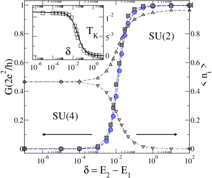
Figure 2: Equilibrium conductance and $T\ll T_{K}$ (left scale) and occupation numbers (right scale) as a function of the level splitting. Squares were obtained by numerical differentiation of the current and circles correspond to Eq. (2). Inset: Kondo temperature as a function of $\delta$. Squares (solid line) correspond to the NCA (analytical) result. Parameters are $\Delta=0.5$. $D=10$, $E_{1}=-4$, $E_{2}=E_{1}+\delta$.

For the numerical calculations, we assume a constant density of states per spin of the leads $\rho$ between $-D$ and $D$ and take $\Gamma=2\Delta=2\pi\rho(V^{\prime})^{2}$ as the unit of energy. Without loss of generality, we take the Fermi level $\epsilon_{F}=E_{s}=0$, and assume $\delta=E_{2}-E_{1}>0$. We also limit our present study to gate voltages that drive the system to the Kondo regime $E_{s}-E_{1}\gg\Delta$, for which the conductance is highest. In Fig. 2 we compare Eq. (2) as a function of $\delta$, with the result obtained by numerical differentiation of the current calculated at very low temperatures (specifically $T=0.05T_{K}(\delta)$, see below). The agreement is very good and gives confidence on the numerical procedure and on the consistency of the NCA results for the current and occupation numbers $n_{i}=2n_{i\sigma}$, also displayed in Fig. 2. We define the Kondo temperature $T_{K}$ as the half width at half maximum of the peak nearest to the Fermi energy of the spectral density $\rho_{1\sigma}(\omega)$ of the lowest doublet. As it is apparent from the inset in Fig. 2, we find that to a high degree of accuracy $T_{K}=fT_{K}^{V}$, where $f$ is a factor of the order of 1 (0.606 for the parameters of Fig. 2), and $T_{K}^{V}$ is given by the following expression

$$T_{K}^{V}=\left\{(D+\delta)D\exp\left[\pi E_{1}/(2\Delta)\right]+\delta^{2}/4\right\}^{1/2}-\delta/2,$$ (3)

obtained minimizing the energy of the simple variational wave function

$$|\psi\rangle=\alpha|s\rangle+\sum_{ik\sigma}\beta_{ik}|i\sigma\rangle\langle 0|c_{ik\sigma}|S\rangle,$$

where $|S\rangle$ is the many-body singlet state with the filled Fermi sea of conduction electrons and the state $|0\rangle$ at the localized site.

Eq. (3) interpolates between both one-level SU(N) limits, $T_{K}^{V}=D\exp\left[\pi E_{1}/(N\Delta)\right]$ ($N=4$ for $\delta=0$ and $N=2$ for $\delta\rightarrow+\infty$). Roughly, $T_{K}(\delta)$ remains constant at the SU(4) value $T_{K}(0)$ ($0.016$ for the parameters of Fig. 2) as long as $\delta<$ $T_{K}(0)$, and then decreases nearly exponentially (by almost two orders of magnitude for $\delta=1$) before flattening at the one-level SU(2) value. As it is apparent in Fig. 2, $T_{K}(0)$ is also the characteristic energy scale for the variation of the conductance with $\delta$, for $T=V=0$. For $\delta$ one order of magnitude less than $T_{K}(0)$, $G_{0}$ is very small, while for $\delta\gg T_{K}(0)$, $G_{0}$ approaches the ideal value for one SU(2) doublet, $2e^{2}/h$.

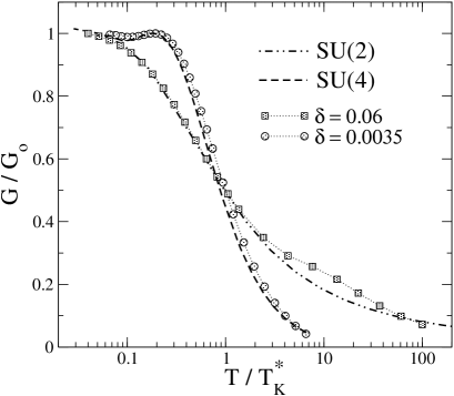
Figure 3: Equilibrium conductance as a function of temperature for several level splittings. Dashed [dashed-dot] line corresponds to the limit of one-level SU(4) [SU(2)] Anderson model. Other parameters as in Fig. 2. For $\delta=0.0035$, $G_{0}=0.08$ and $T_{K}^{*}=0.0137$, while for $\delta=0.06$, $G_{0}=0.97$ and $T_{K}^{*}=0.0025$.

In Fig. 3, we show the evolution with temperature of the conductance for several values of the level splitting $\delta$. Note that the ordinate axis is normalized by $G_{0}$ and the abscissa by $T_{K}^{*}$, the value of the temperature for which $G(T)=G(0)/2$. As expected $T_{K}^{*}\sim T_{K}$. Both $G_{0}$ and $T_{K}^{*}$ have a strong variation with $\delta$. Near the SU(4) limit $\delta\rightarrow 0$, $G_{0}$ is much smaller, but $T_{K}$ is much larger; therefore $G(T)$ persists nearly constant for a much wider range of temperatures. Instead, in the one-level SU(2) limit of large $\delta$, $G(T)$ starts near ideal values but decays much faster with temperature. Near the SU(4) limit, the temperature dependence of the conductance is quite similar to that calculated for the simpler geometry of carbon nanotubes with one particle in the quantum dot cnano , although in the present case, the magnitude is much smaller. The bump observed in the curve for $\delta=0.06$ is due to the contribution of the excited doublet at energy $E_{2}$.

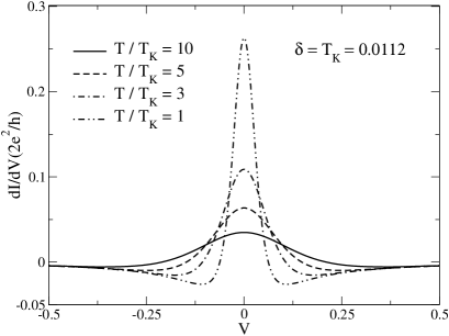
Figure 4: Differential conductance as a function of bias voltage at different temperatures for $\delta=0.0112$. Other parameters as in Fig. 2.

In Fig. 4, we show the non-equilibrium differential conductance as a function of bias voltage $V$ for a level splitting $\delta$ that corresponds to an intermediate region between the SU(4) and one-level SU(2) limits ($\delta\sim T_{K}\sim 0.01$), and for several temperatures. One observes negative $G(V)$ for voltages above the characteristic energy scale $\delta\sim T_{K}$. Our interpretation of this result is the following. Since $\delta\sim T_{K}$, there is only a partial effect of the interference at small bias voltages, and the lowest lying doublet plays a dominant role. However as the energy of the bias voltage $eV$ increases beyond the level splitting $\delta$, both doublets contribute with nearly equal weight to the current, but in opposite ways due to destructive interference. Therefore, the current starts to decrease as the effect of the excited doublet increases for larger applied bias voltages.

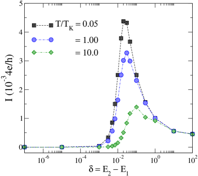
Figure 5: Current as a function of level splitting $\delta$ for $eV=T_{K}^{4}=0.016$ and different temperatures proportional to $T_{K}(\delta)$. Other parameters as in Fig. 2.

In Fig. 5, we display the current as a function of $\delta$ for a fixed bias voltage at low temperatures. The bias voltage was chosen to correspond to the characteristic energy $T_{K}(0)$ of the SU(4) limit. Remarkably, a non monotonic behavior of the current is obtained due to two competing effects. One would expect a monotonous increase of the current with the level splitting as a consequence of the weakening of the destructive interference. However, the Kondo temperature $T_{K}$ decreases strongly with $\delta$, and for a fixed bias voltage a reduction of $T_{K}$ implies a decrease in the current: at low $V$ and $T=0$, for one level with SU(N) symmetry, $G(V)=dI/dV$ has a peak of width of the order of $2T_{K}/e$. Therefore the current at bias voltages which exceed a few $T_{K}/e$ is roughly proportional to $T_{K}$.

We have studied the finite temperature and non equilibrium transport properties of an effective impurity Anderson model containing two doublets, which describes the low-energy physics of quantum interference in nanoscopic systems. In the Kondo regime, dramatic changes in the values of the conductance and its temperature dependence take place as the doublet level splitting is changed by some external parameter. For total destructive interference, the model interpolates between the SU(4) Anderson model when the splitting of the two doublets is $\delta=0$, and the usual SU(2) model for large $\delta$. In the Kondo regime, while the characteristic temperature $T_{K}$ increases significantly towards the SU(4) limit, both, the equilibrium conductance (gate voltage $V=0$) and the total current at finite gate voltages vanish due to destructive interference. For finite $V$ the total current peaks at finite $\delta$ due to the interplay between interference and Kondo effects and when $\delta\sim T_{K}$, the differential conductance becomes negative due to partial destructive interference.

In summary, by considering the interplay between two relevant effects, i.e. quantum interference and Kondo screening, we have shown the important consequences this can have on transport properties through a great variety of nanoscopic and molecular systems.

This work was partially supported by CONICET, by PIP No 11220080101821 of CONICET, by PICT Nos 2006/483 and R1776 of the ANPCyT, Argentina.

References

- (1) J. Park et al., Nature (London) 417, 722 (2002).
- (2) W. Lian et al., Nature (London) 417, 725 (2002).
- (3) N. Roch et al., Nature 453, 633 (2008).
- (4) J. Parks et al., Science 328, 1370 (2010).
- (5) S. Florens et al., J. Phys. Condens. Matter 23, 243202 (2011).
- (6) B. Venkataraman et al., Nature (London) 442, 904 (2006).
- (7) A.V. Danilov et al., Nano Lett. 8, 1 (2008).
- (8) T. Dadosh et al., Nature (London) 436, 677 (2005).
- (9) D. Cardamone et al., Nano Lett. 6, 2422 (2006).
- (10) S.-H. Ke et al., Nano Lett. 8, 3257 (2008).
- (11) G. Begemann et al., Phys. Rev. B 77, 201406(R) (2008).
- (12) J. Rincón et al., Phys. Rev. Lett. 103, 266807 (2009).
- (13) T. Hatano et al., Phys. Rev. Lett. 106, 076801 (2011).
- (14) F. R. Waugh et al., Phys. Rev. Lett. 75, 705 (1995).
- (15) L. Gaudreau et al., Phys. Rev. Lett. 97, 036807 (2006).
- (16) M. C. Rogge et al., Phys. Rev. B 77, 193306 (2008).
- (17) L. P. Kouwenhoven et al., Phys. Rev. Lett. 65,361 (1990).
- (18) E. A. Jagla and C. A. Balseiro, Phys. Rev. Lett. 70, 639 (1993).
- (19) S. Friederich and V. Meden, Phys. Rev. B 77, 195122 (2008).
- (20) K. Hallberg et al., Phys. Rev. Lett. 93, 067203 (2004).
- (21) J. Rincón, et al., Phys. Rev. B 79, 035112 (2009).
- (22) M. H. Hettler et al., Phys. Rev. Lett. 90, 076805 (2003).
- (23) A. M. Lobos and A. A. Aligia, Phys. Rev. Lett. 100, 016803 (2008).
- (24) T. Kuzmenko et al., Phys. Rev. Lett. 96, 046601 (2006)
- (25) V. Meden and F. Marquardt, Phys. Rev. Lett. 96, 146801 (2006).
- (26) H. A. Nilsson et al., Phys. Rev. Lett. 104, 186804 (2010).
- (27) N. S. Wingreen and Y. Meir, Phys. Rev. B 49, 11040 (1994); M. H. Hettler et al., Phys. Rev. B 58, 5649 (1998)
- (28) P. Roura-Bas and A. A. Aligia, J. Phys. Cond. Matt. 22, 025602 (2010).
- (29) P. Roura-Bas, Phys. Rev. B 81, 155327 (2010)
- (30) T. A. Costi et al., Phys. Rev. B 53, 1850 (1996).
- (31) A. A. Aligia et al., Phys. Rev. Lett. 93, 076801 (2004).
- (32) J. S. Lim et al., Phys. Rev. B 74, 205119 (2006); F. B. Anders et al., Phys. Rev. Lett. 100, 086809 (2008); C. A. Büsser et al., Phys. Rev. B 83, 125404 (2011).
- (33) Y. Meir and N. S. Wingreen, Phys. Rev. Lett. 68, 2512 (1992).
- (34) M. Pustilnik and L. I. Glazman, Phys. Rev. Lett. 87, 216601 (2001).
- (35) D.C. Langreth, Phys. Rev. 150, 516 (1966).