Geometric phase contribution to quantum non-equilibrium many-body dynamics

Abstract

We study the influence of geometry of quantum systems underlying space of states on its quantum many-body dynamics. We observe an interplay between dynamical and topological ingredients of quantum non-equilibrium dynamics revealed by the geometrical structure of the quantum space of states. As a primary example we use the anisotropic XY ring in a transverse magnetic field with an additional time-dependent flux. In particular, if the flux insertion is slow, non-adiabatic transitions in the dynamics are dominated by the dynamical phase. In the opposite limit geometric phase strongly affects transition probabilities. We show that this interplay can lead to a non-equilibrium phase transition between these two regimes. We also analyze the effect of geometric phase on defect generation during crossing a quantum critical point.

Introduction.˝̣—The profound interplay and interrelation of geometry and physics was the focus in both fields since creation of General Theory of Relativity, in which quantities responsible for the geometry of space-time are determined by the physical properties of the matter living in this space and vice versa. The relevant geometry language in this case is a Riemannian geometry. Gauge principle of classical gauge theories found its natural description and nice interpretation in terms of theory of fiber bundles, a subject of differential geometry Nakahara2003 . Monopoles and instantons of the gauge theory have profound topological meanings which is the property of defining fiber bundle. Many of these notions appeared in various condensed matter systems at equilibrium. Thus, defects in He and liquid crystals are classified according to the homotopy theory, certain phase transitions are associated to proliferation of topological defects. Topology plays a vital role in e.g. Hall effects and topological insulators.

Another intriguing phenomena, emerging in quantum mechanics, that relates geometry and physics is the Berry phase. When a Hamiltonian is adiabatically driven, its eigenstates acquire not only the familiar dynamical phase factor, but additionally a phase factor that depends only on the geometry of the phase space of the Hamiltonian, namely the Berry phase Berry1984 . It can be observed in interference experiments and in the Aharonov-Bohm effect. The deep geometrical significance of the Berry phase was revealed as well Simon1983 . Therefore, it is also referred to as the geometric phase. We point that while the Berry phase is usually associated with adiabatic processes, the geometric phases describe transformations of arbitrary eigenstates and are thus not tied to the adiabaticity. In condensed matter probably its most transparent manifestation is in the Haldane phenomena (a presence or absence of the excitation gap in 1D spin chain depending on the value of spins).

Until now all these manifestations of the geometric phase were associated to equilibrium and adiabatic phenomena. Here we demonstrate for the first time a direct relevance of topology and geometry of the quantum space of the many body system for the measurable quantities defining a non-equilibrium evolution of the system far from the adiabatic limit. We show that these effects are very significant in the regions close to the quantum phase transition. We thus demonstrate a profound interplay of geometry and topology of the phase space of the quantum many-body system in its out of equilibrium dynamics.

In equilibrium, a Riemannian structure is introduced to quantum mechanics by the Quantum Geometric Tensor (QGT) Provost1980 ,VZ . The QGT $Q_{\mu\nu}$ is defined for an arbitrary eigenstate $|{n}\rangle$ by

$$Q_{\mu\nu}({\boldsymbol{\lambda}},|{n}\rangle):=\langle{n}|\overleftarrow{\partial_{\mu}}\partial_{\nu}|{n}\rangle-\langle{n}|\overleftarrow{\partial_{\mu}}|{n}\rangle\langle{n}|\partial_{\nu}|{n}\rangle,$$ (1)

for $\mu,\nu=1,\ldots,p$, labeling the system’s parameters $\lambda_{\mu}$ which form a manifold $\mathcal{M}$. Its real part is a Riemannian metric tensor $\mathsf{g}_{\mu\nu}$ on ${\mathcal{M}}$ that is related to the fidelity susceptibility which describes the systems response to a perturbation and therefore is an important quantity, e.g. in the study of Quantum Phase Transitions (QPT) VZ . The imaginary part is related to the 2-form (Berry curvature) $F_{\mu\nu}:=\partial_{\mu}A_{\nu}-\partial_{\nu}A_{\mu}=2\Im Q_{\mu\nu},$ where $A_{\mu}({\boldsymbol{\lambda}},|{n}\rangle):=i\langle{n}|\partial_{\mu}|{n}\rangle$ is the connection 1-form. Geometric phase Berry1984 of the state $|{n}\rangle$ is given by its integral along a closed loop $\mathcal{C}$ in parameter space $\gamma_{n}=\int_{\mathcal{C}}A_{\mu}d\lambda^{\mu}$. It is easy to check that after a simple gauge transformation, the Schrödinger equation $i\dot{|{\psi}\rangle}={\hat{\mathrm{H}}}|{\psi}\rangle$ written in the instantaneous basis $|{n}\rangle$ such that $|{\psi}\rangle=\sum_{n}a_{n}|{n}\rangle$ can be put into the following form:

$$\dot{a}_{n}=-\sum_{m\neq n}M_{nm}\exp\left[iE_{nm}(t)-i\Gamma_{nm}(t)\right]\,a_{m},$$ (2)

where $M_{nm}=\langle n|\partial_{t}|m\rangle$. This equation highlights the competition between the dynamical phase $E_{nm}(t)=\int_{0}^{t}\left[\epsilon_{n}(\tau)-\epsilon_{m}(\tau)\right]d\tau$ and the geometric phase $\Gamma_{nm}(t)=\int_{0}^{t}\left[A_{\tau}(|{n}\rangle)-A_{\tau}(|{m}\rangle)\right]d\tau$.

The main purpose of the present work is to demonstrate how geometric effects shows up in quantum dynamics. We do it using an example of a driven XY-model which we introduce in the next paragraph. Generalizations of some of our results to more generic setups are discussed in the Supplementary Information. The main findings of our paper is that geometric phase effects on transition probabilities are small for slow nearly adiabatic driving protocols, i.e. that the leading non-adiabatic transitions are determined by the dynamical phase. Contrary, in the fast limit geometric phase strongly affects transitions between different levels. We also found that the interplay of geometric and dynamical phases can lead to non-equilibrium phase transitions causing sharp singularities in density of excited quasi-particles and pumped energy as a function of the driving velocity. This quantum-critical behavior can happen without undergoing by the system an actual quantum phase transition in the instantaneous basis Carollo2005 . In the limit of slowly driving the system through a quantum critical point with an additional rotation in the parameter space we find that the geometric phase modifies the scaling of the observables with the driving velocity and enhances non-adiabatic effects.

The rotated XY spin chain.—Let us consider a standard, although rich and illustrative example of XY ring in a transverse magnetic field. The Hamiltonian of this system Barouch1970 ; Bunder1999 is defined by

$${\hat{\mathrm{H}}}_{0}=-\sum_{l=1}^{N}\left[\frac{1+g}{2}{\hat{\mathrm{\sigma}}}_{l}^{x}{\hat{\mathrm{\sigma}}}_{l+1}^{x}+\frac{1-g}{2}{\hat{\mathrm{\sigma}}}_{l}^{y}{\hat{\mathrm{\sigma}}}_{l+1}^{y}+h{\hat{\mathrm{\sigma}}}_{l}^{z}\right]$$ (3)

with periodic boundary conditions, i.e., ${\hat{\mathrm{\sigma}}}_{N+1}^{\alpha}={\hat{\mathrm{\sigma}}}_{1}^{\alpha}$. The number of spins $N$ is assumed to be even and the spin $1/2$ on the site $l$ is represented by the usual Pauli matrices ${\hat{\mathrm{\sigma}}}_{l}^{\alpha}$, with $\alpha\in\{x,y,z\}$. Further, the anisotropy for the nearest neighbor spin-spin interaction along the $x$ and $y$ axis is described by the parameter $g$ and $h$ denotes the magnetic field along the $z$ axis.

At $g=0$ this Hamiltonian has an additional $U(1)$ symmetry related to spin-rotations in the $XY$-plain. At finite $g$ this symmetry is broken. Clearly there is a continuous family of ways breaking this symmetry yielding the identical spectrum. The corresponding Hamiltonians are related by applying a unitary rotation of all the spins around the $z$ axis by angle $\phi$:

$${\hat{\mathrm{H}}}(g,h,\phi)={\hat{\mathrm{R}}}(\phi,z){\hat{\mathrm{H}}}_{0}(g,h){\hat{\mathrm{R}}}^{\dagger}(\phi,z),$$ (4)

with the rotation operator ${\hat{\mathrm{R}}}(\phi,z)=\prod_{l=1}^{N}\exp(-i\frac{\phi}{2}{\hat{\mathrm{\sigma}}}_{l}^{z})$. This transformation yields non-trivially complex instantaneous eigenstates, which is a necessary condition for existence of the nontrivial geometric phase Griffiths1994 .

The Hamiltonian (4) can be diagonalized using the Jordan-Wigner and the Fourier transformations:

$${\hat{\mathrm{H}}}(g,h,\phi)=-\sum_{k}\nolimits{\hat{\mathbf{c}}}_{k}^{\dagger}{\hat{\mathrm{H}}}_{k}^{\phantom{\dagger}}{\hat{\mathbf{c}}}_{k}^{\phantom{\dagger}},$$ (5)

with ${\hat{\mathrm{H}}}_{k}=(h-\cos p_{k}){\hat{\mathrm{\sigma}}}^{z}+g\sin p_{k}(\sin 2\phi{\hat{\mathrm{\sigma}}}^{x}-\cos 2\phi{\hat{\mathrm{\sigma}}}^{y})$, ${\hat{\mathbf{c}}}_{k}^{\dagger}=({\hat{\mathrm{c}}}_{-k}^{\phantom{\dagger}},{\hat{\mathrm{c}}}_{k}^{\dagger})$, $p_{k}=\frac{2\pi k}{N}$, $k=\pm 1,\pm 2,\ldots,\pm\frac{N}{2}$ and ${\hat{\mathrm{c}}}_{k}$ are the Fourier transforms of the fermionic operators resulting from the Jordan-Wigner transformation (see Ref. sachdev_book for details). By applying the Bogoliubov transformation to (5) we can map it to a free fermionic Hamiltonian with the known spectrum $\epsilon_{k}(g,h)=\sqrt{(h-\cos p_{k})^{2}+g^{2}\sin^{2}p_{k}}$.

The set of quantum critical points of this spin chain are determined by the vanishing of the energy gap: $2\epsilon_{k_{0}}=0$, where $k_{0}$ is defined by minimizing the excitation energy $\partial_{k}\epsilon_{k}=0$. This condition defines quantum critical regions on $\mathcal{M}$. For the model (4) the gap vanishes on the line ($g=0$, $-1\leq h\leq 1$), marking the anisotropic transition and on the two planes ($g\in\mathbb{R}$, $h=\pm 1$), identifying the Ising transitions damle_96 ; Bunder1999 . The anisotropic transition line belongs to the Lifshitz universality class since it manifests the critical exponents $\nu_{1}=1/2$ and $z_{1}=2$. On the other hand the Ising transition planes belong to the $d=2$ Ising universality class with the critical exponents $\nu_{2}=1$ and $z_{2}=1$ damle_96 . The points where the critical line and the critical plane cross are multicritical points. In Fig. 1 we depict the equilibrium phase diagram of the rotated XY spin chain in the parameter space $(g,h,\phi)$.

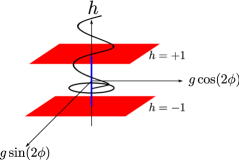
Figure 1: The phase diagram of the rotated XY spin chain in a transverse magnetic field in cylindrical coordinates: The two red planes ($h=\pm 1$) indicate the Ising critical plane, (i.e. the associated QPT belongs to the $d=2$ Ising universality class). Whereas the blue line ($g=0$) marks the anisotropic transition line. The black bold circle and helix describe the two driving protocols we use in this paper.

Dynamics of the rotated XY spin chain.—We explore two driving protocols. The first one is driving the spin rotation $\phi(t)$ with a constant velocity. This corresponds to circular paths in parameter space (see Fig. 1). It is the simplest situation in which a non-trivial geometric phase emerges. The second driving protocol consists of driving the magnetic field $h(t)$ and the spin rotation $\phi(t)$. This results in helical paths in parameter space (Fig. 1) and allows us to study the cross over from the well known Landau-Zener scenario (no geometric phase) to the rotating driving regime (non-trivial geometric phase).

For either of the protocols we assume $\phi(t)=\omega t$ in the time interval $0<t<t_{f}$, where $\omega>0$ is the rate of change of the spin rotation. Then the Schrödinger equation for the coefficients $a_{1,k}$ and $a_{2,k}$, that appear in the expansion of state in the instantaneous basis, $|{\psi}\rangle_{k}=a_{1,k}|{\mathrm{gs}}\rangle_{k}+a_{2,k}|{\mathrm{es}}\rangle_{k}$, becomes a system of linear differential equations with constant coefficients that can be solved exactly (see the Supplementary Information). From this solution we compute the probability for finding the system in the excited state

$$p_{\mathrm{ex},k}=\mathinner{\lvert a_{2,k}(\phi_{f})\rvert}^{2}=\mathsf{g}_{\phi\phi}(|{\mathrm{gs}}\rangle_{k})\frac{\sin^{2}\left[\frac{1}{2}\Omega_{k}(\omega)\phi_{f}\right]}{\left[\frac{1}{2}\Omega_{k}(\omega)\right]^{2}}.$$ (6)

Here $\Omega_{k}(\omega):=\sqrt{\left[\frac{\Delta\epsilon_{k}}{\omega}-\Delta A_{\phi,k}\right]^{2}+4\mathsf{g}_{\phi\phi}(|{\mathrm{gs}}\rangle_{k})}$, $\Delta\epsilon_{k}:=\epsilon_{\mathrm{es},k}-\epsilon_{\mathrm{gs},k}=2\epsilon_{k}$ is the energy difference between the excited and ground states of the $k$-th subspace and $\Delta A_{\phi,k}:=A_{\phi}(|{\mathrm{es}}\rangle_{k})-A_{\phi}(|{\mathrm{gs}}\rangle_{k})$ designates the corresponding difference of the connection 1-forms: $A_{\phi}(|{\mathrm{gs}}\rangle_{k})=i{}_{k}\langle{\mathrm{gs}}|\partial_{\phi}|{\mathrm{gs}}\rangle_{k}$ and $A_{\phi}(|{\mathrm{es}}\rangle_{k})=i{}_{k}\langle{\mathrm{es}}|\partial_{\phi}|{\mathrm{es}}\rangle_{k}$. Further, $\mathsf{g}_{\phi\phi}(|{\mathrm{gs}}\rangle_{k})$ is the Riemannian metric tensor of the $k$-th ground state, which also defines the fidelity susceptibility along the $\phi$ direction:

$$\mathsf{g}_{\phi\phi}(|{\mathrm{gs}}\rangle_{k})=-{}_{k}\langle{\mathrm{gs}}|\partial_{\phi}|{\mathrm{es}}\rangle_{k}{}_{k}\langle{\mathrm{es}}|\partial_{\phi}|{\mathrm{gs}}\rangle_{k}=\left|{}_{k}\langle{\mathrm{es}}|\partial_{\phi}|{\mathrm{gs}}\rangle_{k}\right|^{2}.$$

With this the total density of excited quasi-particles and the energy density of excitations of the entire spin chain in the thermodynamic limit can be calculated by

$$n_{\rm{ex}}=\int_{-\pi}^{\pi}\frac{dk}{2\pi}p_{\mathrm{ex},k},\qquad\epsilon_{\mathrm{ex}}=\int_{-\pi}^{\pi}\frac{dk}{2\pi}2\epsilon_{k}p_{\mathrm{ex},k}.$$ (7)

Before proceeding with the detailed analysis of these two quantities let us make some qualitative remarks on Eq. (6). (i) For the quench of infinitesimal amplitude $\phi_{f}\to 0$ both geometric and dynamical phases are not important and the transition probability is simply given by the product of the square of the quench amplitude and the fidelity susceptibility in agreement with general results degrandi_10 . (ii) In the slow limit $\omega\ll\Delta\epsilon_{k}$ and fixed $\phi_{f}\gtrsim 1$ the geometric phase is still not important while the dynamical phase suppresses the transitions between levels such that $p_{\mathrm{ex},k}\propto\mathsf{g}_{\phi\phi}(|{\mathrm{gs}}\rangle_{k})\omega^{2}/\epsilon_{k}^{2}$. This result is again in perfect agreement with the general prediction for linear quenches in the absence of geometric phase degrandi_10 given that in this case $\omega$ is the velocity of the quench. (iii) The most interesting and nontrivial situation where the geometric phase strongly affects the dynamics occurs when both the rotation frequency and rotation angle are not small: $\omega\gtrsim\Delta\epsilon_{k}$, $\phi_{f}\gtrsim 1$. In particular, in the limit $\omega\to\infty$ and $\phi_{f}=\pi n$ we recover $p_{\mathrm{ex},k}=0$. This trivial physical fact that infinitely fast rotation can not cause transitions between levels actually comes from the mathematical identity: $(\Delta A_{\phi,k})^{2}+4\mathsf{g}_{\phi\phi}(|{\mathrm{gs}}\rangle_{k})=[{\rm Tr}(\partial_{\phi})]^{2}=4$. For large but finite $\omega$ and $\phi_{f}=\pi n$, we find

$$p_{\mathrm{ex},k}\approx\mathsf{g}_{\phi\phi}(|{\mathrm{gs}}\rangle_{k})\sin^{2}\left[\frac{\Delta\epsilon_{k}\Delta A_{\phi,k}}{2\omega}\phi_{f}\right].$$ (8)

If the rotation angle is not large $n\sim 1$ we see that the transition probability in this case is directly proportional to the square of the product of the geometric and dynamical phase differences between the ground and excited states:

$$p_{\mathrm{ex},k}\approx\mathsf{g}_{\phi\phi}(|{\mathrm{gs}}\rangle_{k})\left[\frac{\Delta E_{k}\Delta\gamma_{\phi,k}}{4\pi}\right]^{2},$$ (9)

where $\Delta\gamma_{\phi,k}=\Delta A_{\phi,k}\phi_{f}=\int_{0}^{\phi_{f}}A_{\phi,k}d\phi$ and $\Delta E_{k}=\Delta\epsilon_{k}T$; $T=2\pi/\omega$ is the rotation period. In the limit of large rotation angle at fixed frequency $\Delta E_{k}\ll 1$ and $\phi_{f}\Delta E_{k}\gg 1$ the expression for the transition probability saturates at a value independent of the geometric and dynamical phases: $p_{\rm ex}\sim\mathsf{g}_{\phi\phi}(|{\mathrm{gs}}\rangle_{k})/2$. Interestingly this probability is entirely determined by the Riemannian metric tensor, i.e. has a purely geometric interpretation.

From the discussion above we see that if we focus on the limit of large $\phi_{f}$ and analyze the transition probability as a function of $\omega$ we expect a smooth crossover between two simple regimes both independent of the geometric phase: $p_{\mathrm{ex},k}\sim\mathsf{g}_{\phi\phi}(|{\mathrm{gs}}\rangle_{k})\omega^{2}/\Delta\epsilon_{k}^{2}$ at $\omega\ll\Delta\epsilon_{k}$ and $p_{\mathrm{ex},k}\sim\mathsf{g}_{\phi\phi}(|{\mathrm{gs}}\rangle_{k})/2$ at $\omega\gg\Delta\epsilon_{k}$. A similar crossover between fast and slow regimes is expected in the many-particle situation. Thus one can naively expect that the influence of the geometric phase on the dynamics in the limit of large $\phi_{f}$ is quite limited. The reality turns out to be much more interesting though as we illustrate below. In this limit we can simplify the $k$ integrals in Eqs. (7) using the stationary phase approximation. Then we find that the resulting behavior of $n_{\rm ex}$ and $\epsilon_{\rm ex}$ exhibits a “cusp” at a critical driving velocity $\omega_{c}$ determined by $\omega_{c}=1-h$. This is illustrated in Fig. 2.

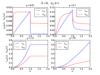
Figure 2: A plot of the total density of excited quasi-particles (red line) and the energy density of excitations (blue line) as a function of the rotation frequency $\omega$ in the limit of many rotations $\phi_{f}\gg 1$ and for vanishing magnetic field $h=0$, with different anisotropy $g=0.01,0.1,1.0,10$, showing a cusp at the critical driving velocity $\omega_{c}=1$, which can be interpreted as a “dynamical quantum phase transition”.

Because this singularity is recovered via the stationary phase method we expect it to be valid for a class of models with similar Hamiltonians. This cusp and the associated “dynamical quantum phase transition” is directly related to the effect of geometric phase. To understand this let us apply a unitary transform ${\hat{\mathrm{U}}}_{k}(t)=\mathop{\mathrm{diag}}(e^{+i\phi(t)},e^{-i\phi(t)})$, to go into a rotating frame, where the geometric phase is removed from the Hamiltonian. The resulting Hamiltonian in the rotating frame reads ${\hat{\mathrm{H}}}_{k,\mathrm{rot}}=\left[\left(h-\cos p_{k}\right)+\partial_{t}\phi\right]{\hat{\mathrm{\sigma}}}^{z}+g\sin p_{k}\left(\sin 2\phi{\hat{\mathrm{\sigma}}}^{x}-\cos 2\phi{\hat{\mathrm{\sigma}}}^{y}\right)$, where the spectrum takes the following form $\epsilon_{k,\mathrm{rot}}=\sqrt{(h+\omega-\cos p_{k})^{2}+g^{2}\sin^{2}p_{k}}$. From the spectrum we see that the Hamiltonian in the rotated frame has a quantum phase transition at $h+\omega_{c}=1$. This transition gives raise to the cusp in Fig. 2. We note though that the emergence of the cusp is non-trivial since by quenching rotation frequency we are pumping finite energy density to the system. In the equilibrium this model does not have any singularities at finite temperature. Thus this singularity is a purely non-equilibrium phenomenon. Further, Fig. 2 illustrates nicely that for a small $g$ the regime where $n_{\mathrm{ex}}$ and $\epsilon_{\mathrm{ex}}$ saturate with $\omega$ is close to $\omega_{c}$. However for $g>1$ the dependence of the saturation point on $g$ is approximated numerically as $\omega_{\mathrm{sat}}(g,h=0)=51.7g^{0.54}+21.8g^{1.35}$.

Another possibility to analyze the interplay of geometric and dynamical phases on excess energy and density of excitations is to consider the following helical driving protocol: $(h(t)=\delta\,t,\phi(t)=\omega\,\delta\,t)$, beginning in the ground state at $t_{i}=0$ and stopping at $t_{f}=\frac{2}{\delta}$, i.e. crossing a quantum critical point. Now $\delta$ plays the role of driving velocity, both in $h$ and, for $\omega\neq 0$, in circular directions and $\omega$ determines the helicity of the path.

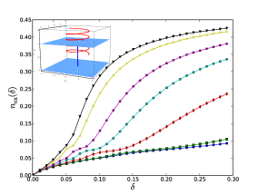
Figure 3: Landau-Zener to Helix: The density of excited quasi-particles is plotted as a function $\delta$ the driving velocity for different helicities $\omega=0,0.9,3,5,7,10,12$ (from down to the top) with $N=300$ spins and an anisotropy of $g=0.9$. For non zero $\omega$ we observe linear scaling regime with $\delta$.

For $\omega=0$ we realize the usual Landau-Zener protocol and for $\omega>0$ we describe a helical path in the parameter space. In Fig. 3 we present the density of excitations obtained from an exact numerical integration of the time-dependent Schrödinger equation. We recover (Fig. 3) for $\omega=0$ (lowest curve) the scaling $n_{\mathrm{ex}}\sim\sqrt{\delta}$, as expected by the Kibble-Zurek scaling argument Polkovnikov2005 ; zurek2005 . With increasing $\omega$ the density of excitations makes a crossover to a different linear scaling regime with $\delta$. However, in accord with our general discussion in the strict adiabatic limit we always observe $n_{\rm ex}\propto\sqrt{\delta}$.

Conclusion.—In summary, we addressed how the geometric phase influences quantum many-body non-equilibrium dynamics. We showed that at intermediate of fast driving regimes geometric phase strongly affects transition probabilities between levels. We showed that a dynamical quantum phase transition can emerge as a result of a competition between the geometric and dynamical phases. This transition manifests itself in the “cusp” in the driving velocity dependence of various observables (like e.g. the density of excitation and the energy density) at finite energy. This allows us to probe quantum criticalities “from a distance”, without actually crossing them. Such a possibility should be attractive from an experimental point of view since the system doesn’t need to undergo a QPT. We also found that the geometric phase modifies the scaling with the driving velocity as compared to the LZ scaling. This can be related to effective topology-induced interaction between the defects. This effect is stronger in the gap-less regions of the phase diagram. We also note that our results rely only on the geometry of the phase space and thus rather generic. We expect that they extend to other protocols where one applies a time-dependent unitary transformation to the Hamiltonian or other transformation which involves nontrivial geometric phase. In particular, similar considerations apply to the Dicke model realized in Ref. Esslinger . This and possible other generalizations of our results (e.g. for open Tomadin2011 or turbulent Nowak2011 systems) will be discussed in a separate work.

Appendix A Supplementary Information

Appendix B Effective Hamiltonian in the rotating frame

Let us consider a more general setup, which extends the example studied in the main text. Suppose that the system is described by some interacting Hamiltonian $\mathcal{H}_{0}$, which is rotationally invariant with respect to some vector coupling ${\boldsymbol{\lambda}}$ . This coupling can represent, for example, an external magnetic or electric field, anisotropic interaction constant, couple to a nematic order parameter etc. It can also break an internal $\mathrm{U}(1)$ symmetry of $\mathcal{H}_{0}$ like the mixing symmetry between different spin components. At nonzero value of ${\boldsymbol{\lambda}}$ the rotational symmetry is thus broken. Now let us consider a dynamical process where this coupling uniformly rotates at a fixed magnitude. Then the time dependent Hamiltonian reads

$$\mathcal{H}(t)=U^{-1}(t)\mathcal{H}({\boldsymbol{\lambda}}_{0})U(t),$$ (10)

where $U(t)$ is the unitary operator corresponding to this rotation. In the rotating frame $|\tilde{\psi}(t)\rangle=U|\psi(t)\rangle$ the effective Hamiltonian in the Schrödinger equation picks up an additional “centrifugal” term:

$$i\hbar\partial_{t}|\tilde{\psi}\rangle = \mathcal{H}_{\rm eff}|\tilde{\psi}\rangle,$$ (11)

$$\mathcal{H}_{\rm eff} = \mathcal{H}(\lambda_{0})-i\hbar\omega U^{-1}\partial_{\phi}U,$$ (12)

where $\phi$ is the rotational angle and $\omega=\dot{\phi}$ is the frequency. The centrifugal term in the Hamiltonian has a number of interesting properties. (i) It is proportional to the frequency $\omega$ and thus can be used to continuously modify the effective Hamiltonian. (ii) At constant frequency the effective Hamiltonian is time independent. (iii) The diagonal components of the centrifugal term are given by the connection 1-form of the corresponding energy levels. Let us point that the time independence of the centrifugal term, which follows its rotational invariance, and its locality imply that the rotations in the generic parameter space do not lead to the continuous heating even in ergodic non-integrable systems. This situation is opposite to e.g. Floquet Hamiltonians. Which are usually non-local and lead to constant energy absorption in generic interacting systems. Thus we expect that the qualitative results of the Paper are valid even if we add arbitrary interactions to the Hamiltonian, which preserve the rotational symmetry but break its integrability.

Appendix C Derivation of Eq. (6)

Here we show how Eq. (6) in the main text can be obtained for a generic two-level system using only the minimal assumption that time dependence enters through some $\mathrm{U}(1)$ rotation with constant frequency. For such a system the Schrödinger equation in the instantaneous basis $\{|{\mathrm{gs}}\rangle,|{\mathrm{es}}\rangle\}$ can be written as

$$\partial_{t}\tilde{a}_{\mathrm{gs}} =-\langle{\mathrm{gs}}|\partial_{t}|{\mathrm{es}}\rangle\exp\left[iE_{\mathrm{gs},\mathrm{es}}(t)-i\Gamma_{\mathrm{gs},\mathrm{es}}(t)\right]\tilde{a}_{\mathrm{es}},$$ (13)

$$\partial_{t}\tilde{a}_{\mathrm{es}} =-\langle{\mathrm{es}}|\partial_{t}|{\mathrm{gs}}\rangle\exp\left[iE_{\mathrm{es},\mathrm{gs}}(t)-i\Gamma_{\mathrm{es},\mathrm{gs}}(t)\right]\tilde{a}_{\mathrm{gs}},$$ (14)

where $E_{nm}(t)$ and $\Gamma_{nm}(t)$ are the dynamical and geometric phases as defined in the main text. Notice that we applied the gauge transformation $a_{n}=\tilde{a}_{n}\exp\left[\int_{ti}^{t}\mathrm{d}\tau\left(-i\epsilon_{n}(\tau)+iA_{\tau}(|{n}\rangle)\right)\right]$ to the coefficients introduced by: $|{\psi(t)}\rangle=a_{\mathrm{gs}}(t)|{\mathrm{gs}(t)}\rangle+a_{\mathrm{es}}(t)|{\mathrm{es}(t)}\rangle$. In agreement with the discussion in the previous section all matrix elements appearing in the Schrödinger equation (13), (14) are time independent for the angle linearly changing in time $\phi(t)=\omega t$. It is convenient to change variables from time $t$ to the angle $\phi$ in (13), (14):

$$\partial_{\phi}\tilde{a}_{\mathrm{gs}}=-\langle{\mathrm{gs}}|\partial_{\phi}|{\mathrm{es}}\rangle\exp\left[i\frac{E_{\mathrm{gs},\mathrm{es}}(\phi)}{\omega}-i\Gamma_{\mathrm{gs},\mathrm{es}}(\phi)\right]\tilde{a}_{\mathrm{es}},$$ (15)

$$\partial_{\phi}\tilde{a}_{\mathrm{es}}=-\langle{\mathrm{es}}|\partial_{\phi}|{\mathrm{gs}}\rangle\exp\left[i\frac{E_{\mathrm{es},\mathrm{gs}}(\phi)}{\omega}-i\Gamma_{\mathrm{es},\mathrm{gs}}(\phi)\right]\tilde{a}_{\mathrm{gs}},$$ (16)

differentiating Eq. (16) one more time with respect to $\phi$ and eliminating $\tilde{a}_{\mathrm{gs}}$, $\partial_{\phi}\tilde{a}_{\mathrm{gs}}$ gives a second order differential equation with constant coefficients:

$$\partial_{\phi}^{2}\tilde{a}_{\mathrm{es}}-i\left(\frac{\Delta\epsilon}{\omega}-\Delta A_{\phi}\right)\partial_{\phi}\tilde{a}_{\mathrm{es}}+\mathsf{g}_{\phi\phi}(|{\mathrm{gs}}\rangle)\tilde{a}_{\mathrm{es}}=0.$$ (17)

From this it is trivial to derive Eq.(6) from the main text:

$$p_{\mathrm{ex}}=\mathinner{\lvert a_{\mathrm{es}}(\phi_{f})\rvert}^{2}=\mathsf{g}_{\phi\phi}(|{\mathrm{gs}}\rangle)\frac{\sin^{2}\left[\frac{1}{2}\Omega(\omega)\phi_{f}\right]}{\left[\frac{1}{2}\Omega(\omega)\right]^{2}},$$ (18)

with $\Omega(\omega):=\sqrt{\left[\frac{\Delta\epsilon}{\omega}-\Delta A_{\phi}\right]^{2}+4\mathsf{g}_{\phi\phi}(|{\mathrm{gs}}\rangle)}$.

References

- (1) M. Nakahara, Geometry, Topology and Physics, Taylor & Francis, 2003.
- (2) M. V. Berry, Proc. R. Soc. London A 392, 45 (1984).
- (3) B. Simon, Phys. Rev. Lett. 51, 2167 (1983).
- (4) J.P. Provost, G. Vallee, Commun. Math. Phys. 76, 289 (1980)
- (5) L. CamposVenuti, P.Zanardi, Phys. Rev. Lett. 99, 095701 (2007).
- (6) A.C.M. Carollo and J.K. Pachos, Phys. Rev. Lett. 95, 157203 (2005).
- (7) E. Barouch, B. M. McCoy and M. Dresden, Phys. Rev. A 2, 1075, (1970).
- (8) J. E. Bunder and Ross H. McKenzie, Phys. Rev. B 60, 344, (1999)
- (9) D. Griffiths, Introduction to Quantum Mechanics, Prentice Hall, 1994.
- (10) S. Sachdev, Quantum Phase Transitions (Cambridge University Press, Cambridge, 1999).
- (11) K. Damle and S. Sachdev, Phys. Rev. Lett. 76, 4412 (1996).
- (12) C. De Grandi, V. Gritsev, A. Polkovnikov, Phys. Rev. B 81, 012303 (2010).
- (13) A. Polkovnikov, Phys. Rev. B. 72, 161201(R) (2005).
- (14) W. H. Zurek, U. Dorner, P. Zoller, Phys. Rev. Lett. 95, 105701 (2005).
- (15) K. Baumann, C. Guerlin, F. Brennecke and T. Esslinger, Nature 464, 1301 (2010).
- (16) A. Tomadin, S. Diehl, and P. Zoller, Phys. Rev. A 83, 013611, (2011).
- (17) B. Nowak, D. Sexty, and T. Gasenzer, Phys. Rev. B 84, 020506(R), (2011).