Abstract

It has been shown recently that the normal branch of a DGP braneworld scenario self-accelerates if the induced gravity on the brane is modified in the spirit of $f(R)$ modified gravity. Within this viewpoint, we investigate cosmological viability of the Hu-Sawicki type modified induced gravity. Firstly, we present a dynamical system analysis of a general $f(R)$-DGP model. We show that in the phase space of the model, there exist three standard critical points; one of which is a de Sitter point corresponding to accelerating phase of the universe expansion. The stability of this point depends on the effective equation of state parameter of the curvature fluid. If we consider the curvature fluid to be a canonical scalar field in the equivalent scalar-tensor theory, the mentioned de Sitter phase is unstable, otherwise it is an attractor, stable phase. We show that the effective equation of state parameter of the model realizes an effective phantom-like behavior. A cosmographic analysis shows that this model, which admits a stable de Sitter phase in its expansion history, is a cosmologically viable scenario.
PACS: 04.50.-h, 98.80.-k
Key Words: Braneworld Cosmology, Phantom Mimicry, Dynamical System, Cosmography

1 Introduction

The late-time accelerating phase of the universe expansion which is supported by data related to the luminosity measurements of high red shift supernovae [1], measurements of degree-scale anisotropies in the cosmic microwave background (CMB) [2] and large scale structure (LSS) [3], is one of the challenging problems in the modern cosmology. The rigorous treatment of this phenomenon can be provided essentially in the framework of general relativity. In the expression of general relativity, late time acceleration can be explained either by an exotic fluid with large negative pressure that is dubbed as dark energy in literature, or by modifying the gravity itself which is dubbed as dark geometry or dark gravity proposal. The first and simplest candidate of dark energy is the cosmological constant, $\Lambda$ [4]. But, there are theoretical problems associated with it, such as its unusual small numerical value (the fine tuning problem), no dynamical behavior and even its unknown origin [5]. These problems have forced cosmologists to introduce alternatives in which dark energy evolves during the universe evolution. Scalar field models with their specific features provide an interesting alternative for cosmological constant and can reduce the fine tuning and coincidence problems. In this respect, several candidate models have been proposed: quintessence scalar fields [6], phantom fields [7] and Chaplygin gas [8] are among these candidates. Nevertheless, we emphasize that the scalar field models of dark energy are not free of shortcomings.

As an alternative for dark energy, modification of gravity can be accounted for the late time acceleration. Among the most popular modified gravity scenarios which may successfully describe the cosmic speed-up, is $f(R)$ gravity [9,10]. Modified gravity also can be achieved by extra-dimensional theories in which the observable universe is a 4-dimensional brane embedded in a five-dimensional bulk. The Dvali-Gabadadze-Porrati (DGP) model is one of the extra-dimensional models that can describe late-time acceleration of the universe in its self-accelerating branch due to leakage of gravity to the extra dimension [11,12].

Recent observations constrain the equation of state parameter of the dark energy to be $w_{X}\approx-1$ and even $w_{X}<-1$ [13]. One of the candidates for dark energy of this kind is the phantom scalar field. This component has the capability to create the mentioned acceleration and its behavior is extremely fitted to observations. But it suffers from theoretical problems; it violates the null energy condition and its energy density increases with expansion of the universe leading to a future big rip singularity. Also it causes the quantum vacuum instabilities. So, some authors have attempted to realize a kind of phantom-like behavior ($w_{eff}<-1$) in the cosmological models without introduction of phantom fields. In fact, the possibility of realization of an effective phantom nature without introduction of phantom fields is an important task and has been appreciated sufficiently in recent years [14].

In the streamline of the mentioned issues, we are going to study cosmological viability of a class of DGP-inspired braneworld models in which the induced gravity on the normal branch is modified in the spirit of $f(R)$ gravity [10,15,16,17]. Firstly, we study the cosmological dynamics of this model within a dynamical system approach. We show that there exists a standard de Sitter point in the phase plane of the model. In this respect, this model has the potential to explain accelerated expansion of the universe. The stability of this point depends completely on the effective equation of state parameter of the curvature fluid. If we consider the curvature fluid to be a canonical scalar field in the equivalent scalar-tensor theory, the mentioned de Sitter phase is unstable, otherwise it is an attractor, stable phase. Since the late-time accelerating phase of the universe expansion is explained by a stable de Sitter phase, we can investigate the cosmological viability of such theoretical models based on the phantom-like behavior of this $f(R)$-DGP gravity. To be more specific, in which follows we focus on the cosmological viability of the Hu-Sawicki type modified induced gravity and show that this model has capability to realize a stable, attractor de Sitter phase. We point out that the phantom mimicry discussed in this study has a geometric origin. To be more realistic, we compare our results with observation via a cosmographic approach.

2 $f(R)$-DGP scenario

In this section, possible modification of the induced gravity on the brane is investigated in the spirit of $f(R)$ theories [10,15,16,17]. It has been shown that $4D$ $f(R)$ theories in the present time can follow closely the expansion history of the $\Lambda$CDM universe [18]. Here we study an extension of $f(R)$ theories to a DGP braneworld setup. The motivation behind this study is that modified induced gravity on the normal branch of a DGP scenario provides some new interesting features, one of which is self-acceleration of the normal DGP branch in this situation (see Refs. [10,16,17] for details). Similar to the normal branch of the standard DGP cosmology, the resulting generalized normal branch is also ghost-free and therefore the issue of ghost-instabilities is irrelevant in this case [17]. The action of this model can be written as follows

$${\cal{S}}=\frac{M_{5}^{3}}{2}\int d^{5}x\sqrt{-g}{\cal{R}}+\int d^{4}x\sqrt{-q}\Big{(}M_{5}^{3}\overline{K}+{\cal{L}}\Big{)}\,,$$ (1)

where by definition

$${\cal{L}}=\frac{m_{p}^{2}}{2}f(R)+{\cal{L}}_{m}\,.$$ (2)

By calculating the bulk-brane Einstein’s equations and using a spatially flat FRW line element, the following modified Friedmann equation is obtained [15,16,17]

$$H^{2}=\frac{8\pi G}{3}\bigg{(}\rho^{(m)}+\rho^{(rad)}+\rho^{(curv)}\bigg{)}\pm\frac{H}{\bar{r}_{c}}$$ (3)

where

$$\rho^{(curv)}=m_{p}^{2}\bigg{(}\frac{1}{2}\Big{[}f(R)-Rf^{\prime}(R)\Big{]}-3\dot{R}Hf^{\prime\prime}(R)\bigg{)}\,,$$ (4)

is energy density corresponding to the curvature part of the theory. This energy density can be dubbed as dark curvature energy density. $\bar{r}_{c}$ is the re-scaled crossover distance that is defined as $\bar{r}_{c}=r_{c}f^{\prime}(R)$ and a prime marks differentiation with respect to the Ricci scalar, $R$. We note that in this scenario there is an effective gravitational constant, which is re-scaled by $f^{\prime}(R)$ so that $G=G_{eff}\equiv\frac{1}{8\pi m_{p}^{2}f^{\prime}(R)}$ [15]. In order to study the phase space of this scenario, it is more suitable to rewrite the normal branch of the Friedmann equation (3) in the following more phenomenological form

$$E^{2}=\Omega_{m}(1+z)^{3}+\Omega_{rad}(1+z)^{4}+\Omega_{curv}(1+z)^{3(1+w_{curv})}-2\sqrt{\Omega_{r_{c}}}E\,,$$ (5)

where by definition

$$\Omega_{curv}=\frac{8\pi G}{3H_{0}^{2}}\rho_{0}^{(curv)}\,\,,\quad\quad\Omega_{r_{c}}=\frac{1}{4[r_{c}f_{0}^{\prime}(R)]^{2}H_{0}^{2}}\,,$$

and also

$$w_{curv}=-1+\frac{\ddot{R}f^{\prime\prime}(R)+\dot{R}\Big{[}\dot{R}f^{\prime\prime\prime}(R)-Hf^{\prime\prime}(R)\Big{]}}{\frac{1}{2}[f(R)-Rf^{\prime}(R)]-3H\dot{R}f^{\prime\prime}(R)}\,.$$ (6)

We note that $w_{curv}$ is not a constant and varies with redshift.

3 The phase space of a general $f(R)$-DGP model

To investigate cosmological dynamics of this model within a dynamical system approach, we express the cosmological equations in the form of an autonomous, dynamical system. For this purpose, we define the following normalized expansion variables

$$p=\frac{\sqrt{\Omega_{m}}}{a^{3/2}E}\,,\quad\quad r=\frac{\sqrt{\Omega_{rad}}}{a^{2}E}\,,\quad\quad s=\frac{\sqrt{\Omega_{curv}}}{a^{3(1+w_{curv})/2}E}\,,\quad\quad u=\frac{\sqrt{\Omega_{r_{c}}}}{E}\,.$$ (7)

In this way, equation (5) with minus sign (corresponding to the generalized normal DGP branch) and in a dimensionless form, is written as follows

$$1+2u=p^{2}+r^{2}+s^{2}\,.$$ (8)

This constraint means that the allowable phase space of this scenario in the $p$-$r$-$s$ space is outside of a sphere with radius $1$, which is defined as $p^{2}+r^{2}+s^{2}\geq 1$ . The autonomous system is obtained as follows

$$\left\{\begin{array}[]{ll}p^{\prime}=\frac{3p\Big{[}p^{2}+(1+2w_{curv})r^{2}+\frac{5}{3}s^{2}-1\Big{]}}{2(p^{2}+r^{2}+s^{2}+1)}\,,\vspace{0.5cm}\\ r^{\prime}=\frac{3r\Big{[}2p^{2}+\frac{8}{3}s^{2}+(1+w_{curv})(r^{2}-p^{2}-s^{2}-1)\Big{]}}{2(p^{2}+r^{2}+s^{2}+1)}\,,\vspace{0.5cm}\\ s^{\prime}=\frac{s\Big{[}2s^{2}+p^{2}+(1+3w_{curv})r^{2}-2\Big{]}}{p^{2}+r^{2}+s^{2}+1}\,.\end{array}\right.$$ (9)

Here a prime marks differentiation with respect to the new time variable $\tau=\ln{a}$ that $a$ is scale factor of the universe. The critical points in the phase plane are obtained by solving the equations $p^{\prime}=0$, $r^{\prime}=0$ and $s^{\prime}=0$, that is, setting the autonomous system (9) to be vanishing. The results are shown in table 1. To investigate the stability of these points, we apply the linear approximation analysis to achieve the Jacobian matrix. Note that the critical points and their stability depend on the value of $w_{curv}$ . Here we investigate the stability of the standard critical points in two different subspaces of the model parameter space where EoS of the curvature fluid has either a phantom or a quintessence character. As we see in table 1, the radiation dominated phase (point $A$) and matter dominated phase (point $B$) in this scenario, are unstable phases of the universe expansion independent on the value of $w_{curv}$ . Whereas, the accelerating phase of the universe expansion (point $C$) is a stable phase if the curvature fluid is considered to be a non-canonical (phantom) scalar field ($w_{curv}<-1$) in equivalent scalar-tensor theory; otherwise it is an unstable phase. It is necessary to mention that whenever $w_{curv}=-1$, the variables $s$ and $u$ are not independent and the phase space is $2$D (here the curvature fluid plays the role of a cosmological constant, the same as $\Lambda DGP$ model. For more details see Ref. [19]). Figure 1 shows the $3$D phase space trajectories of the model. In this figure, the point $C$ as a de Sitter point is an attractor for $w_{curv}<-1$. Therefore, a model universe which is described by modified induced gravity on the normal DGP branch, has a stable, positively accelerated expansion phase if the modified gravity indicates a phantom-like behavior. We note that points $O$ and $C^{\prime}$ do not belong to physical phase space of our model universe.

After exploration of the cosmological dynamics in a general $f(R)$-DGP setup within a phase space analysis, in the next section we study cosmological viability of an specific $f(R)$-DGP model.

Table 1: Eigenvalues and the stability properties of the critical points.

points	$(p,r,s)$	character	eigenvalues	$w_{curv}<-1$	$w_{curv}>-1$
$A$	$(0,0,1)$	radiation	$\Big{[}2\,,\frac{1}{2}(1-3w_{curv})\,,\frac{1}{2}\Big{]}$	unstable	unstable
$B$	$(1,0,0)$	matter	$\Big{[}-\frac{1}{2}\,,-\frac{3}{2}w_{curv}\,,\frac{3}{2}\Big{]}$	unstable	unstable
$C$	$(0,1,0)$	de Sitter	$\Big{[}\frac{3w_{curv}-1}{2}\,,\frac{3(1+w_{curv})}{2}\,,\frac{3(1+4w_{curv})}{8}$]	stable	unstable

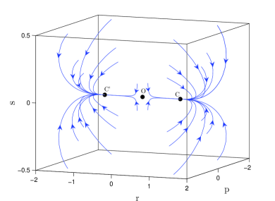
Figure 1: The $3$D phase space of the autonomous system (9) for $w_{curv}<-1$. There are three critical points: $C$ is an attractor de Sitter point, $O$ is a saddle point and $C^{\prime}$ is an attractor point.

4 Cosmological viability of the Hu-Sawicki type modified induced gravity

Now we focuss on the cosmological viability of the model by considering a Hu-Sawicki type modified induced gravity on the DGP brane. It is shown in the Ref. [18] that the expansion history of the mentioned model in $4$ dimensions is widely close to the $\Lambda$CDM model in the high-redshift regime. Now in a braneworld extension, we expect the Hu-Sawicki induced gravity mimics the $\Lambda$DGP model in the mentioned regime. In other words, in this regime curvature term in the Friedmann equation is close to the cosmological constant which is screened by the term $\frac{H}{\bar{r}_{c}}$ . In fact, the dynamical screening effect is the main origin of the phantom-like behavior of the curvature term in the normal branch of this DGP-inspired braneworld scenario [15]. The Hu-Sawicki model [18] is given by

$$f(R)=R-m^{2}\,\frac{c_{1}(\frac{R}{m^{2}})^{n}}{c_{2}(\frac{R}{m^{2}})^{n}+1},$$ (10)

where $m^{2}$, $c_{1}$, $c_{2}$ and $n$ are free positive parameters that can be expressed as functions of density parameters. Now we explore the dependence of these parameters on density parameters defined in our setup. Variation of the action (1) with respect to the metric yields the induced modified Einstein equations on the brane

$$G_{\alpha\beta}=\frac{1}{M_{5}^{6}}{\cal{S}}_{\alpha\beta}-{\cal{E}}_{\alpha\beta}\,,$$ (11)

where ${\cal{E}}_{\alpha\beta}$ (which we neglect it in our forthcoming arguments), is the projection of the bulk Weyl tensor on the brane

$${\cal{E}}_{\alpha\beta}=^{(5)}C_{RNS}^{M}\,n_{M}n^{R}g_{\alpha}^{N}g_{\beta}^{S}$$ (12)

and ${\cal{S}}_{\alpha\beta}$ as the quadratic energy-momentum correction into Einstein field equations is defined as follows

$${\cal{S}}_{\alpha\beta}=-\frac{1}{4}\tau_{\alpha\mu}\tau^{\mu}_{\beta}+\frac{1}{12}\tau\tau_{\alpha\beta}+\frac{1}{8}g_{\alpha\beta}\tau_{\mu\nu}\tau^{\mu\nu}-\frac{1}{24}g_{\alpha\beta}\tau^{2}\,.$$ (13)

$\tau_{\alpha\beta}$ as the effective energy-momentum tensor localized on the brane is defined as [10]

$$\tau_{\alpha\beta}=-m_{p}^{2}f^{\prime}(R)G_{\alpha\beta}+\frac{m_{p}^{2}}{2}\Big{[}f(R)-Rf^{\prime}(R)\Big{]}g_{\alpha\beta}+T_{\alpha\beta}+m_{p}^{2}\Big{[}\nabla_{\alpha}\nabla_{\beta}f^{\prime}(R)-g_{\alpha\beta}\Box f^{\prime}(R)\Big{]}\,.$$ (14)

The trace of Eq. (11), which can be interpreted as the equation of motion for $f^{\prime}(R)$ , is obtained as

$$R=\frac{5}{24M_{5}^{6}}\tau^{2}\,.$$ (15)

$\tau$, the trace of the effective energy-momentum tensor localized on the brane is expressed as

$$\tau=m_{p}^{2}\Big{[}2f(R)-Rf^{\prime}(R)-3\Box f^{\prime}(R)\Big{]}-(\rho_{m}+\rho_{rad})\,,$$ (16)

To highlight the DGP character of this generalized setup, we express the results in terms of the DGP crossover scale defined as $r_{c}=\frac{m_{p}^{2}}{2M_{5}^{3}}$. So, the equation of motion for $f^{\prime}(R)$ is rewritten as follows

$$\frac{5}{6}r_{c}^{2}\Bigg{(}\Big{[}2f(R)-Rf^{\prime}(R)\Big{]}^{2}+9\Big{(}\Box f^{\prime}(R)\Big{)}^{2}+6Rf^{\prime}(R)\Box f^{\prime}(R)-12f(R)\Box f^{\prime}(R)\Bigg{)}$$

$$+\frac{5}{6}\frac{r_{c}}{M_{5}^{3}}\Big{[}Rf^{\prime}(R)-2f(R)+3\Box f^{\prime}(R)\Big{]}(\rho_{m}+\rho_{rad})+\frac{5}{24M_{5}^{6}}(\rho_{m}+\rho_{rad})^{2}-R=0\,.$$ (17)

In the next stage, we solve this equation for $\Box f^{\prime}(R)$ to obtain

$$\Box f^{\prime}(R)=-\frac{1}{3}\Bigg{[}\Big{(}Rf^{\prime}(R)-2f(R)\Big{)}+\frac{\rho_{m}+\rho_{rad}}{2M_{5}^{3}\,r_{c}}\Bigg{]}\pm\frac{1}{r_{c}}\sqrt{\frac{2R}{15}}\,,$$ (18)

Now we introduce an effective potential $V_{eff}$ which satisfies $\Box f^{\prime}(R)=\frac{\partial V_{eff}}{\partial f^{\prime}(R)}\,$. This effective potential has an extremum at

$$\Big{[}Rf^{\prime}(R)-2f(R)\Big{]}+\frac{1}{m_{p}^{2}}(\rho_{m}+\rho_{rad})=\pm\frac{1}{r_{c}}\sqrt{\frac{6}{5}R}\,.$$ (19)

In the high-curvature regime, where $f^{\prime}(R)\simeq 1$ and $\frac{f(R)}{R}\simeq 1$ , we recover the standard DGP result (one can compare this result with corresponding result obtained in Ref. [18] to see the differences in this extended braneworld scenario)

$$R\pm\frac{1}{r_{c}}\sqrt{\frac{6}{5}R}=\frac{1}{m_{p}^{2}}\,(\rho_{m}+\rho_{rad})\,.$$ (20)

The negative and positive signs in this equation are corresponding to the DGP self-accelerating and normal branches respectively. In which follows, we adopt the positive sign corresponding to the normal branch of the scenario. To investigate the expansion history of the universe in this setup, we restrict ourselves to those values of the model parameters that yield expansion histories which are observationally viable. We note that the Hu-Sawicki $f(R)$ function introduced in Ref. [18], was interpreted as a cosmological constant in the high-curvature regime. The motivation for that interpretation was to obtain a $\Lambda$CDM behavior in the high curvature (in comparison with $m^{2}$) regime. Here we show that in a braneworld extension, the Hu-Sawicki induced gravity mimics the $\Lambda$DGP model in the mentioned regime. As we have pointed out previously, the phantom-like behavior can be realized from the dynamical screening of the brane cosmological constant. In this respect, we apply the same strategy to our model, so that the second term in the Hu-Sawicki $f(R)$ function (that is, the second term in the right hand side of equation (10)) mimics the role of an effective cosmological constant on the DGP brane. Then this term will be screened by $\frac{H}{\overline{r}_{c}}$ term in the late time (see the normal branch of Eq. (3)).

In the case in which $R\gg m^{2}$ , one can approximate Eq. (10) as follows

$$\lim_{\frac{m^{2}}{R}\rightarrow 0}f(R)\approx R-\frac{c_{1}}{c_{2}}m^{2}+\frac{c_{1}}{c_{2}^{2}}m^{2}\Big{(}\frac{R}{m^{2}}\Big{)}^{n}.$$ (21)

During the late-time acceleration epoch, $f^{\prime}_{0}(R)\simeq 1$ or equivalently $R_{0}\gg m^{2}$ and we can apply the above approximation. Also the curvature field is always near the minimum of the effective potential. So, based on Eq. (19), we have

$$R+\frac{1}{r_{c}}\sqrt{\frac{6}{5}R}=\frac{1}{m_{p}^{2}}\,(\rho_{m}+\rho_{rad})+2\frac{c_{1}}{c_{2}}m^{2}\,.$$ (22)

Since $R$ in the $f(R)$ function is induced Ricci scalar on the brane, we except crossover scale to affect on the constant parameters $c_{1}$ , $c_{2}$ and $m^{2}$. In Ref. [18] the authors obtained $3m^{2}\equiv R_{c}=\frac{\rho_{0m}}{m_{p}^{2}}$ that $\rho_{0m}$ is the present value of the matter density. But, in our setup the present value of the matter density (see Eq. (20)) is given by

$$R_{c}+0.9\frac{\sqrt{R_{c}}}{r_{c}}=\frac{1}{m_{p}^{2}}\,(\rho_{0m}+\rho_{0rad})\,.$$ (23)

If we solve this equation for $R_{c}$, we find

$$3m^{2}\equiv R_{c}\approx\Omega_{r_{c}}+3\Omega_{m}+3\Omega_{rad}\pm 3\sqrt{\Omega_{r_{c}}\Big{(}0.068\Omega_{r_{c}}+\Omega_{m}+\Omega_{rad}\Big{)}}\,.$$ (24)

Therefore, the DGP character of this extended modified gravity scenario is addressed through $m^{2}$. As we have mentioned, at the curvatures high compared with $m^{2}$, the second term on the right hand side of equation (10) mimics the role of an effective cosmological constant on the brane. In this respect, the second term in the right hand side of equation (21) also mimics the role of a cosmological constant on the brane in the high curvature regime. With this motivation, we find

$$\frac{c_{1}}{c_{2}}\approx\frac{18\Omega_{\Lambda}}{\Omega_{r_{c}}+3\Omega_{m}+3\Omega_{rad}\pm 3\sqrt{\Omega_{r_{c}}\Big{(}0.068\Omega_{r_{c}}+\Omega_{m}+\Omega_{rad}\Big{)}}}\,.$$ (25)

There is also a relation for $\frac{c_{1}}{c_{2}^{2}}$ as follows

$$\frac{c_{1}}{c_{2}^{2}}=\frac{1-f_{0}^{\prime}(R)}{n}\bigg{(}\frac{R_{0}}{m^{2}}\bigg{)}^{n+1}\,,$$ (26)

where $\frac{R_{0}}{m^{2}}$ in our setup can be calculated as follows: firstly, by using Eqs. (22) and (25), we find

$$R+\frac{1}{r_{c}}\sqrt{\frac{6}{5}R}=\frac{1}{m_{p}^{2}}\,(\rho_{{}_{0}m}a^{-3}+\rho_{0rad}\,a^{-4})+12\Omega_{\Lambda}\,,$$ (27)

where $\rho_{{}_{0}m}$ can be omitted through Eq. (23) to obtain

$$R+\frac{1}{r_{c}}\sqrt{\frac{6}{5}R}=\bigg{(}3m^{2}+1.56\frac{m}{r_{c}}-\frac{1}{m_{p}^{2}}\,\rho_{0rad}\bigg{)}a^{-3}+\frac{1}{m_{p}^{2}}\,\rho_{0rad}\,a^{-4}+12\Omega_{\Lambda}\,.$$ (28)

Finally, if we solve this equation for $\sqrt{R}$ , we find the following relation for $\frac{R_{0}}{m^{2}}$

$$\frac{R_{0}}{m^{2}}\approx\Bigg{(}-\frac{0.9\sqrt{\Omega_{r_{c}}}}{m}+\bigg{[}3\Big{(}1+\frac{0.52\sqrt{\Omega_{r_{c}}}}{m}\Big{)}^{2}+\frac{12\Omega_{\Lambda}}{m^{2}}\bigg{]}^{1/2}\Bigg{)}^{2}\,,$$ (29)

where $m$ is given by Eq. (24). Note that we have set $H_{0}$ and $a(t_{0})$ equal to unity. These relations tell us that the free parameters of this model are $n$, $\Omega_{m}$, $\Omega_{rad}$, $\Omega_{r_{c}}$ and $f_{0}^{\prime}(R)$, whereas the latter one is constrained by the Solar-System tests. In fact, experimental data show that $f^{\prime}(R)-1~{}<10^{-6}$ , when $f^{\prime}(R)$ is parameterized to be exactly  $1$  in the far past. To analyze the behavior of $w_{curv}$ , we specify the following ansatz for the scale factor

$$a(t)=\bigg{(}t^{2}+\frac{t_{0}}{1-\nu}\bigg{)}^{\frac{1}{1-\nu}}\,,$$ (30)

where $\nu\neq 1$ is a free parameter [20]. By noting that the Ricci scalar is $R=6(\frac{\ddot{a}}{a}+(\frac{\dot{a}}{a})^{2})$, one can express the function $f(R)$ of equation (10) in terms of the redshift $z$. Figure $2$ shows the variation of the effective equation of state parameter versus the redshift. As we see in this figure, in this class of models the curvature fluid has an effective phantom-like equation of state, $w_{curv}<-1$, at high redshifts and then approaches the phantom divide ($w_{curv}=-1$) at a redshift that increases by decreasing $n$.

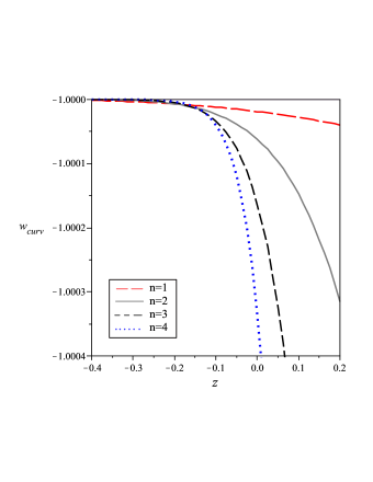
Figure 2: $w_{curv}$ versus the redshift for a Hu-Sawicki type modified induced gravity with $\Omega_{m}=0.27$,  $\Omega_{rad}=0.3$,  $\Omega_{\Lambda}=0.9$,  $\Omega_{r_{c}}=0.01$ and $f_{0}^{\prime}(R)-1\approx 10^{-6}$ . As this figure shows, in this class of models the curvature fluid has an effective phantom equation of state with $w_{curv}<-1$ at high redshifts. This effective equation of state parameter approaches the phantom divide line ($w_{curv}=-1$) at a redshift that increases by decreasing the values of $n$.

The main point here is that a modified induced gravity of the Hu-Sawicki type in the DGP framework, gives an effective phantom-like equation of state parameter for all values of $n$, and all of these models approach asymptotically to the de Sitter phase ($w_{curv}=-1$). Therefore, the accelerated expansion of the universe (the de Sitter phase) is necessarily a stable attractor phase for this DGP-inspired $f(R)$ model. Based on the analysis presented in the previous section within a phase space viewpoint and also the outcomes of this section, we can conclude that a Hu-Sawicki type modified induced gravity on the normal branch of the DGP setup provides a cosmologically viable scenario. This is the case since it contains a radiation dominated era followed by a matter dominated era and finally a stable de Sitter phase in its expansion history. In the next section we compare our model with observational data via a cosmographic analysis. Our treatment here is mainly based on the Ref. [29,30].

5 Comparison with observational data

While theoretical consistency of a physical theory is a primary condition for viability of the theory, the observational consistency of the model is necessary too. For this goal, in which follows we discuss briefly observational status of our model via a cosmographic analysis. Before that, we note that the DGP model is a testable scenario with the same number of parameters as the standard $\Lambda$CDM model, and has been constrained from many observational data, such as the SNe Ia data set [21], the baryon mass fraction in clusters of galaxies from the X-ray gas observation [22], CMB data [23], the large scale structures [24] and the baryon acoustic oscillation (BAO) peak [25], the observed Hubble parameter $H(z)$ data [26], the gravitational lensing surveys [27]. The observational constraints on the DGP model with Gamma-ray bursts (GRBs) at high redshift also obtained recently from the Union2 Type Ia supernovae data set [28]. In [28] the authors are shown that by combining the GRBs at high redshift with the Union2 data set, the WMAP7 results, the BAO observation, the clusters baryon mass fraction, and the observed Hubble parameter data set and also in order to favor a flat universe, the best fit of the density parameter values of the DGP model are obtained as $\{\Omega_{m},\Omega_{r_{c}}\}=\{0.235_{-0.014}^{+0.015}\,\,,0.138_{-0.048}^{+0.051}\}$ [28].

Here to compare our $f(R)$-DGP model with observational data we adopt the cosmography approach. Cosmography approach is a useful tool in order to constrain higher order gravity observationally without need to solve field equations or addressing complicated problems related to the growth of perturbations [29,30]. In this case, one can define cosmographic parameters based on the fifth order Taylor expansion of the scale factor. One can also relate the characteristic quantities defining the $f(R)$-DGP model to the mentioned cosmographic parameters. Therefore, a measurement of the cosmographic parameters makes it possible to put constraints on $f(R_{0})$ and its first three derivatives. The likelihood function for the probe $s$ is defined as [31]

$${\cal{L}}_{s}(\textbf{p})\propto\exp{(-\chi_{s}^{2}(\textbf{p})/2)}$$ (31)

where

$$\chi_{s}^{2}(\textbf{p})=\sum_{n=1}^{{\cal{N}}_{s}}\frac{\Big{[}\mu_{obs}(z_{i})-\mu_{th}(z_{i},\textbf{p})\Big{]}^{2}}{\sigma_{\mu_{i}}(z_{i})}$$ (32)

$\mu_{obs}(z_{i})$ are the observed distance modulus for the adopted standard candle (such as SNe Ia) at the redshift $z_{i}$ with its error $\sigma_{\mu_{i}}$.  $\mu_{th}(z)$ are the theoretical values of the distance modulus from cosmological models which read as $\mu_{th}(z,\textbf{p})=25+5\log{D_{L}(z,\textbf{p})}$  where $D_{L}=H_{0}d_{L}$ is the luminosity distance. In the cosmography approach, one can obtain an analytical expression for luminosity distance versus the cosmographic parameters so that one require no priori model to solve $d_{L}=(1+z)\int_{{}_{0}}^{{}^{z}}\frac{dz^{\prime}}{E(z^{\prime})}$ . By using the least squares fitting that means the getting of $\chi_{s\,min}^{2}$, one can obtain the suitable cosmographic parameters. In the next step, one should relate the $f(R)$ function and its first three derivatives to the cosmographic parameters to set constraints on the parameters of the $f(R)$ function [29,30]. In this manner we constrain observationally the parameters of a Hu-Sawicki type $f(R)$ induced gravity on the normal DGP brane by the cosmography approach. Our strategy in this cosmographic approach is mainly based on the recent paper by Bouhmadi-Lòpez et al. [30]. Firstly we relate the functions $f(R_{0})$, $f^{\prime}(R_{0})$, $f^{\prime\prime}(R_{0})$ and $f^{\prime\prime\prime}(R_{0})$ to the parameters $R_{0}$, $\dot{R}_{0}$, $\ddot{R}_{0}$,  $(\frac{d^{3}R}{dt^{3}})_{0}$ and $\dot{H}_{0}$ which are expressed versus the cosmographic parameters by using the Friedmann and Raychaudhuri equations at $t=t_{0}$ . Now we have a system of two equations with four unknowns. To expand the $f(R)$ function and its derivatives versus these cosmographic parameters, we need to two further equations to close the system. In 4-dimensional $f(R)$ gravity, the Newtonian gravitational constant $G$ is replaced by an effective (time dependent) quantity as $G_{eff}=\frac{G}{f^{\prime}(R)}$. On the other hand, it is reasonable to assume that the present day value of $G_{eff}$ is the same as the Newtonian one $G_{eff}(z=0)=G$ or $f^{\prime}(R_{0})\simeq 1$ . One may note that the Hu-Sawicki model with this condition reduces to the Einstein-Hilbert gravity with Lagrangian $f(R)=R$. In order to resolve this problem, we can replace the condition $f^{\prime}(R_{0})=1$ with $f^{\prime}(R_{0})=(1+\epsilon)^{-1}$. Another relation can also be obtained by differentiating the Raychaudhuri equation [29,30]. We solve this system of four equations for four unknowns to obtain the following relations

$$\left\{\begin{array}[]{ll}\frac{f(R_{0})}{6H_{0}^{2}}=-\frac{{\cal{A}}_{0}\Omega_{m}+{\cal{B}}_{0}+{\cal{C}}_{0}(r_{c}H_{0})^{-1}}{\cal{D}}+\epsilon(2-q_{0})\,,\vspace{0.5cm}\\ \frac{f^{\prime\prime}(R_{0})}{(6H_{0}^{2})^{-1}}=-\frac{{\cal{A}}_{2}\Omega_{m}+{\cal{B}}_{2}+{\cal{C}}_{2}(r_{c}H_{0})^{-1}}{\cal{D}}+\epsilon\frac{{\cal{B}}_{2}-{\cal{C}}^{\prime}_{2}}{\cal{D}}\,,\vspace{0.5cm}\\ \frac{f^{\prime\prime\prime}(R_{0})}{(6H_{0}^{2})^{-2}}=-\frac{{\cal{A}}_{3}\Omega_{m}+{\cal{B}}_{3}+{\cal{C}}_{3}(r_{c}H_{0})^{-1}}{(j_{0}-q_{0}-2)\cal{D}}+\epsilon\frac{{\cal{B}}^{\prime}_{3}-{\cal{C}}^{\prime}_{3}}{(j_{0}-q_{0}-2)\cal{D}}\,,\end{array}\right.$$ (33)

where ${\cal{A}}_{i}$, ${\cal{B}}_{i}$, ${\cal{C}}_{i}$ and $\cal{D}$ with $i=0,2,3$ are functions of $q_{0}$, $j_{0}$, $s_{0}$ and $l_{0}$ (these functions are defined in Ref. [30]). The new quantities ${\cal{C}}^{\prime}_{2}$, ${\cal{B}}^{\prime}_{3}$, and ${\cal{C}}^{\prime}_{3}$ are defined as follows

$${\cal{C}}^{\prime}_{2}=j_{0}(j_{0}-q_{0}^{2}-1)+q_{0}(q_{0}^{2}+q_{0}-3)-2\,,\quad$$ (34)

$${\cal{B}}^{\prime}_{3}=2j_{0}(2q_{0}^{2}+6q_{0}+j_{0}+3)+2q_{0}(15q_{0}^{2}+42q_{0}+39)$$

$$-2l_{0}(1+q_{0})-2s_{0}(q_{0}+j_{0})+24\,,\quad$$ (35)

$${\cal{C}}^{\prime}_{3}=j_{0}\big{(}-j_{0}+[2q_{0}+8]q_{0}+s_{0}+7\Big{)}+s_{0}(1-q_{0}^{2})$$

$$-q_{0}\Big{(}q_{0}[q_{0}^{2}+8q_{0}-2]-s_{0}-17\Big{)}+8\,.$$ (36)

In the second step we have to determine the values of the cosmographic parameters that have the best fit to the observational data (by the least squares fitting). Instead, here we use a minimal approach to parameterize the cosmographic parameters by the phenomenological density parameters. In other words, the cosmographic parameters will be calculated for a given phenomenologically parameterized dark energy model. The best choice is the $\Lambda$CDM model. In Ref. [30] the details of these calculations are done. They finally obtained the following results [30]

$$q_{0}=-1+\frac{3}{2}\Omega_{m}\,,\quad\quad j_{0}=1\,,\quad\quad s_{0}=1-\frac{9}{2}\Omega_{m}\,,\quad\quad l_{0}=1+3\Omega_{m}+\frac{27}{2}\Omega_{m}^{2}\,.$$ (37)

Now one can substitute these results into equations (33) and consider the observational conservative values $\Omega_{m}=0.266$ and $\Omega_{r_{c}}=10^{-4}$ where $\Omega_{r_{c}}=(4r_{c}^{2}H^{2}_{0})^{-1}$ [2]. Finally, by considering the first order approximation in $\epsilon$, one obtains the following results

$$\frac{f(R_{0})}{6H_{0}^{2}}=0.849+2.6\epsilon\,,\quad\frac{f^{\prime\prime}(R_{0})}{(6H_{0}^{2})^{-1}}=0.16-20.5\epsilon\,,\quad\frac{f^{\prime\prime\prime}(R_{0})}{(6H_{0}^{2})^{-2}}=1.3+0.0176\epsilon$$ (38)

In the HS model, there are four parameters $c_{1}$, $c_{2}$, $R_{c}$ and $n$ that can be constrained by observational data via the values of the $f(R_{0})$ and its derivatives. So, we should create a system of four equations in the four unknowns through equation (10) and its first three derivatives. By solving equation (10) and its first derivative for $c_{1}$ and $c_{2}$, with $f(R_{0})=0.849+2.6\epsilon$ and $f^{\prime}(R_{0})=(1+\epsilon)^{-1}$ , one finds [29]

$$\widetilde{c}_{1}\equiv c_{1}R_{c}^{1-n}=\frac{n(1+\epsilon)}{\epsilon}R_{0}^{1-n}\bigg{[}1-\frac{0.849+2.6\epsilon}{R_{0}}\bigg{]}^{2}$$ (39)

$$\widetilde{c}_{2}\equiv c_{2}R_{c}^{-n}=\frac{n(1+\epsilon)}{\epsilon}R_{0}^{-n}\bigg{[}1-\frac{0.849+2.6\epsilon}{R_{0}}-\frac{\epsilon}{n(1+\epsilon)}\bigg{]}\,.$$ (40)

By substituting relations (39) and (40) in HS $f(R)$ function and its derivatives, it is obvious that parameter $R_{c}$ cancels out so that we have to work with two parameters $\widetilde{c}_{1}$ and $\widetilde{c}_{2}$ instead of three parameters $c_{1}$, $c_{2}$ and $R_{c}$ . In other words, $R_{c}$ cannot be obtained in this fashion. By setting the second derivative of the HS function equal to $f^{\prime\prime}(R_{0})=0.16-0.5\epsilon$, we get

$$n=\frac{[(0.849+2.6\epsilon)/R_{0}]+[(1+\epsilon)/\epsilon](1-[0.16-0.5\epsilon]/R_{0})-(1-\epsilon)/(1+\epsilon)}{1-(0.849+2.6\epsilon)/R_{0}}\,.$$ (41)

In the last stage and in order to determine the value of $\epsilon$ , one can use the third derivative of the HS function and setting $f^{\prime\prime\prime}(R_{0})=1.3+0.0176\epsilon$ to obtain the following constraint (see also [29])

$$\frac{1.3+0.0176\epsilon}{0.849+2.6\epsilon}=\frac{1+\epsilon}{\epsilon}\frac{(0.16-0.5\epsilon)}{R_{0}}\bigg{[}R_{0}\frac{(0.16-0.5\epsilon)}{0.849+2.6\epsilon}+\frac{\epsilon(0.849+2.6\epsilon)}{1+\epsilon}\Big{(}1-\frac{2\epsilon}{1-(0.849+2.6\epsilon)/R_{0}}\Big{)}\bigg{]}$$ (42)

Using this constrain, the acceptable value of $\epsilon$ is $\simeq 0.03$ (note that there are three other values of $\epsilon$ that are not acceptable since are very large). The value of $R_{0}$ is determined by $R_{0}=6H_{0}^{2}(1+q_{0})$ with $q_{0}=-1+\frac{3}{2}\Omega_{m}$. By equation (41), we get $n\simeq 2$ and by equations (39) and (40) we obtain $\widetilde{c}_{1}\simeq 10$ and $\widetilde{c}_{2}\simeq 0.7$ . Note that as we excepted these parameters are positive. The parameter $R_{c}$ here plays the role of a scaling parameter. We obtain $c_{1}$ and $c_{2}$ from equations (25) and (26) and then by using their relation with $\widetilde{c}_{1}$ and $\widetilde{c}_{2}$, we find $R_{c}\simeq 0.018$  which is a reasonable value for this quantity.

6 Summary

Recently a mechanism to self-accelerate the normal branch of the DGP model, which is known to be free from the ghost instabilities, has been reported [17]. This mechanism is based on the modified induced gravity. In this paper, firstly we studied the cosmological dynamics of this model within a phase space approach. A de Sitter phase is the simplest cosmological solution that exhibits acceleration. As we have shown in a dynamical system viewpoint, this phase appears in our generalized setup. In fact, based on the dynamical system approach, we showed that there exists a de Sitter fixed point in phase space of a general $f(R)$-DGP model. In order to investigate the stability of this accelerating phase of expansion, we classified the $f(R)$ functions in two different subspaces of the model parameter space. We have shown that if the $f(R)$ induced gravity plays effectively the role of a phantom scalar field in the equivalent scalar-tensor theory, it leads to a stable de Sitter solution and these models are cosmologically viable. Then, as an specific model, we studied the Hu-Sawicki type modified induced gravity in the DGP framework and we found that the equation of state parameter of the curvature fluid has an effective phantom-like character. The origin of the phantom-like behavior in the model presented here can be due to the dynamical screening effect of the curvature term (which plays effectively the role of a cosmological constant in high-redshift regime on the brane). In other words, in this case the phantom-like behavior has a pure gravitational origin. We have shown also that the Hu-Sawicki modified induced gravity mimics the $\Lambda$DGP model in the high-redshift regime. Since the Hu-Sawicki modified induced gravity contains an early time radiation dominated era followed by a matter domination era and then a stable de Sitter phase in its expansion history, it is cosmologically a viable scenario. This result is independent on the value of free parameter $n$ of the Hu-Sawicki model. Finally we have tried to constrain our model based on the observational data through a cosmographic procedure. In this manner we obtained reasonable values for parameters of the Hu-Sawicki induced gravity.

Acknowledgement
We would like to thank an anonymous referee for insightful suggestions.

References

-
[1]
S. Perlmutter et al, Astrophys. J. 517 (1999) 565
A. G. Riess et al, Astron. J. 116 (1998) 1006
P. Astier et al, Astron. Astrophys. 447 (2006) 31
W. M. Wood-Vasey et al, Astrophys. J. 666 (2007) 694 -
[2]
A. D. Miller et al, Astrophys. J. Lett. 524 (1999) L1
S. Hanany et al, Astrophys. J. Lett. 545 (2000) L5
D. N. Spergel et al, Astrophys. J. Suppl. 148 (2003) 175
R. Lazkoz and E. Majerotto, JCAP 015 (2007) 0707 [arXiv:0704.2606]. -
[3]
M. Colless et al, Mon. Not. R. Astron. Soc. 328 (2001)
1039
M. Tegmark et al, Phys. Rev. D 69 (2004) 103501
S. Cole et al., Mon. Not. R. Astron. Soc. 362 (2005) 505
V. Springel, C. S. Frenk, and S. M. D. White, Nature (London) 440 (2006) 1137. -
[4]
V. Sahni and A. A. Starobinsky, Int. J. Mod. Phys. D 9 (2000)
373
T. Padmanabhan, Phys. Rept. 380 (2003) 235
E. J. Copeland, M. Sami and S. Tsujikawa, Int. J. Mod. Phys. D 15 (2006) 1753. -
[5]
S. Weinberg, Rev. Mod. Phys. 61 (1989) 1
S. M. Carroll, Living Rev. Relativity 4 (2001) 1
R. R. Caldwell, R. Dave and P. Steinhardt, Phys. Rev. D 59 (1999) 123504. -
[6]
B. Ratra and P. J. E. Peebles, Phys. Rev. D 37 (1988) 3406
T. D. Saini, S. Raychaudhury, V. Sahni and A. A. Starobinsky, Phys. Rev. Lett. 85 (2000) 1162
P. Brax and J. Martin, Phys. Rev. D 61 (2000) 103502
T. Barreiro, E. J. Copeland and N. J. Nunes, Phys. Rev. D 61 (2000) 127301
V. Sahni and L. Wang, Phys. Rev. D 62 (2000) 103517
V. Sahni, M. Sami and T. Souradeep, Phys. Rev. D 65 (2002) 023518
M. Sami, N. Dadhich and T. Shiromizu, Phys. Lett. B 568 (2003) 118
M. Sami and T. Padmanabhan, Phys. Rev. D 67 (2003) 083509. -
[7]
R. R. Caldwell, Phys. Lett. B 545 (2002) 23
S. Tsujikawa and M. Sami, Phys. Lett. B 603 (2004) 113
R. R. Caldwell and E. V. Linder, Phys. Rev. Lett. 95 (2005) 141301. -
[8]
A. Kamenshchik, U. Moschella and V. Pasquier, Phys. Lett. B 511
(2001) 265
A. Dev, J. S. Alcaniz and D. Jain, Phys. Rev. D 67 (2003) 023515
L. Amendola, F. Finelli, C. Burigana and D. Carturan, JCAP 0307 (2003) 005
O. Bertolami, A. A. Sen, S. Sen and P. T. Silva, Mon. Not. Roy. Astron. Soc. 353 (2004) 329
M. Biesiada, W. Godlowski and M. Szydlowski, Astrophys. J. 622 (2005) 28
X. Zhang, F. -Q. Wu and J. Zhang, JCAP 0601 (2006) 003
H. Zhang and Z. -H. Zhu, Phys. Rev. D 73 (2006) 043518
H. Zhang, Z. -H. Zhu and L. Yang, Mod. Phys. Lett. A 24 (2009) 541
M. Roos, [arXiv:0704.0882]; M. Roos, [arXiv:0804.3297]; M. Roos, Phys. Lett. B 666 (2008) 420
M. Bouhmadi-López and R. Lazkoz, Phys. Lett. B 654 (2007) 51. -
[9]
S. Capozziello, V. F. Cardone, S. Carloni and A. Troisi, Int. J.
Mod. Phys. D 12 (2003) 1969
S. Nojiri and S. D. Odintsov, Int. J. Geom. Meth. Mod. Phys. 4 (2007) 115
T. P. Sotiriou and V. Faraoni, Rev. Mod. Phys. 82 (2010) 451.
S. Nojiri and S. D. Odintsov, Gen. Relat. Gravit. 36 (2004) 1765
S. Nojiri and S. D. Odintsov, Class. Quantum Grav. 22 (2005) L35
S. Nojiri and S. D. Odintsov, Phys. Rev. D 74 (2006) 086009
S. Nojiri and S. D. Odintsov, Phys. Rev. D. 78 (2008) 046006
K. Bamba, S. Nojiri and S. D. Odintsov, JCAP 0810 (2008) 045
S. M. Carroll, V. Duvvuri, M. Trodden and M. S. Turner, Phys. Rev. D70 (2004) 043528
L. Amendola, D. Polarski and S. Tsujikawa, Phys. Rev. Lett. 98 (2007) 131302
A. Starobinsky, JETP Lett. 86 (2007) 157
S. Capozziello, S. Nojiri, S. D. Odintsov and A. Troisi, Phys. Lett. B 639 (2006) 135. -
[10]
K. Nozari and M. Pourghassemi, JCAP 10 (2008) 044.
K. Atazadeh, M. Farhoudi and H. R. Sepangi, Phys. Lett. B 660 (2008) 275
J. Saavedra and Y. Vasquez, JCAP 04 (2009) 013 -
[11]
G. R. Dvali, G. Gabadadze and M. Porrati, Phys. Lett. B 484
(2000) 112
C. Deffayet, Phys. Lett. B 502 (2001) 199
A. Lue, Phys. Rept. 423 (2006) 48. -
[12]
G. Dvali, G. Gabadadze and M. Porrati, Phys. Lett. B 485
(2000) 208
G. Dvali and G. Gabadadze, Phys. Rev. D 63 (2001) 065007
G. Dvali, G. Gabadadze, M. Kolanovi and F. Nitti, Phys. Rev. D 65 (2002) 024031. -
[13]
A. Melchiorri, L. Mersini, C. G. Odman and M. Trodden, Phys. Rev. D
68 (2003) 043509
A. G. Riess et al, Astrophs. J. 607 (2004) 665
E. Komatsu et al. [WMAP Collaboration], Astrophys. J. Suppl. 180 (2009) 330, [arXiv:0803.0547]. -
[14]
V. Sahni and Y. Shtanov, JCAP 0311 (2003) 014
V. Sahni, Y. Shtanov, A. Viznyuk, JCAP 0512 (2005) 005
A. Lue and G. D. Starkman, Phys. Rev. D 70 (2004) 101501. - [15] K. Nozari and F. Kiani, JCAP 07 (2009) 010, [arXiv:0906.3806].
- [16] M. Bouhmadi-Lòpez, JCAP 0911 (2009) 011, [ arXiv:0905.1962].
-
[17]
K. Nozari and N. Rashidi, JCAP 0909 (2009) 014,
[arXiv:0906.4263]
K. Nozari and T. Azizi, Phys. Lett. B 680 (2009) 205, [arXiv:0909.0351]
K. Nozari and N. Aliopur, Europhys. Lett. 87 (2009) 69001
K. Atazadeh and H. R. Sepangi, JCAP 0709 (2007) 020
K. Atazadeh and H. R. Sepangi, JCAP 01 (2009) 006. -
[18]
W. Hu and I. Sawicki, Phys. Rev. D 76 (2007) 064004
M. Martinelli, A. Melchiorri anf L. Amendola, Phys. Rev. D 79 (2009) 123516. - [19] L. P. Chimento, R. Lazkoz, R. Maartens and I. Quiros, JCAP 0609 (2006) 004.
- [20] Y. -Fu. Cai, T. Qiu, Y. -S. Piao, M. Li and X. Zhang, JHEP 071 (2007) 0710.
-
[21]
C. Deffayet, S. J. Landau, J. Raux, M. Zaldarriaga and P. Astier,
Phys. Rev. D 66 (2002) 024019
P. P. Avelino and C. J. A. P. Martins, ApJ 565 (2002) 661
Z.-H. Zhu and J. S. Alcaniz, ApJ, 620 (2005) 7
R. Maartens and E. Majerotto, Phys. Rev. D 74 (2006) 023004
V. Barger, Y. Gao and D. Marfatia, Phys. Lett. B 648 (2007) 127. - [22] J. S. Alcaniz and Z. -H. Zhu, Phys. Rev. D 71 (2005) 083513.
-
[23]
R. Lazkoz, R. Maartens and E. Majerotto, Phys. Rev. D 74 (2006)
083510
S. Rydbeck, M. Fairbain and A. Goobar, JCAP 0705 (2007) 003
J.-H. He, B. Wang and E. Papantonopoulos, Phys. Lett. B 654 (2007) 133 -
[24]
T. Multamäki, E. Gaztanaga and M. Manera, MNRAS 344 (2003)
761
A. Lue, R. Scoccimarro and G. D. Starkman, Phys. Rev. D 69 (2004) 124015
K. Koyama and R. Maartens, JCAP 0601 (2006) 016
Y. -S. Song, I. Sawicki and W. Hu, Phys. Rev. D 75 (2007) 064003. - [25] Z. -K. Guo, Z. -H. Zhu, J. S. Alcaniz and Y. -Z. Zhang, Astrophys. J 646 (2006) 1.
- [26] H. Y. Wan, Z. L. Yi, T. J. Zhang and J Zhou, Phys. Lett. B 651 (2007) 352.
- [27] D. Jain, A. Dev and J. S. Alcaniz, Phys. Rev. D 66 (2002) 083511.
- [28] N. Liang, Z. -H. Zhu, Res. Astron. Astrophys, [arxiv:1010.2681].
- [29] S. Capozziello, V. F. Cardone and V. Salzano, Phys. Rev. D 78 (2008) 063504, [arXiv:0802.1583].
- [30] M. Bouhmadi-Lòpez, S. Capozziello and V. F. Cardone, Phys. Rev. D 82 (2010) 103526, [arXiv:1010.1547].
- [31] K. Nozari, T. Azizi and N. Alipour, Mon. Not. R. Astron. Soc. 412 (2011) 2125, [arXiv:1011.3395].