Generation of Seed Magnetic Field around First Stars:
the Biermann Battery Effect

Abstract

We investigate generation processes of magnetic fields around first stars. Since the first stars are expected to form anisotropic ionization fronts in the surrounding clumpy media, magnetic fields are generated by effects of radiation force as well as the Biermann battery effect. We have calculated the amplitude of magnetic field generated by the effects of radiation force around the first stars in the preceding paper, in which the Biermann battery effects are not taken into account. In this paper, we calculate the generation of magnetic fields by the Biermann battery effect as well as the effects of radiation force, utilizing the radiation hydrodynamics simulations. As a result, we find that the generated magnetic field strengths are $\sim 10^{-19}{\rm G}-10^{-17}$G at $\sim 100$pc-1kpc scale mainly by the Biermann battery, which is an order of magnitude larger than the results of our previous study. We also find that this result is insensitive to various physical parameters including the mass of the source star, distance between the source and the dense clump, unless we take unlikely values of these parameters.

1 Introduction

According to the theoretical studies in the last decade, first stars are expected to be very massive ($\gtrsim 100M_{\odot}$) (e.g., Bromm, Coppi & Larson, 2002; Nakamura & Umemura, 2001; Abel, Bryan, Norman, 2002; Yoshida, 2006). Recent studies which properly address the accretion phase of first star formation also revealed that the primary star formed in the center of the mini-halo is not very massive but still massive $\gtrsim 10~{}M_{\odot}$, although significant fraction of first stars are less massive ($\lesssim 1M_{\odot}$)(Stacy et al., 2010; Clark et al., 2011a, b; Greif et al., 2011). In any case, star formation episodes in the very early universe are different from that in local galaxies. One of the reasons of this difference is that the primordial gas clouds that host the first stars lack heavy elements, though they are most efficient coolants in interstellar clouds at $T\lesssim 1000$K. Because of the lack these coolants, the temperature of the primordial gas cloud is kept around $\sim$1000K during its collapse for $n_{\rm H}<10^{12}{\rm cm^{-3}}$, which is much hotter than the local interstellar molecular gas clouds. Consequently, the Jeans mass of the collapsing primordial gas is much larger than that of the interstellar gas, which leads to the formation of very massive stars(e.g., Omukai, 2000).

Another important difference between the star formation sites in the early universe and local molecular clouds is the strengths of magnetic fields. Typical field strength $B\sim 10{\rm\mu G}$ in the local molecular gas results in the formation of jets from protostars and regulate the gravitational collapse of cloud cores. The effects of magnetic field on the star formation in the early universe have been studied from theoretical aspects. First of all, the coupling of the magnetic field with the primordial gas was studied by a detailed chemical reaction model(Maki & Susa, 2004, 2007). They found that magnetic field is basically frozen-in the primordial gas during its collapse, differently from the local interstellar gas(e.g., Nakano & Umebayashi, 1986a, b). Under the assumption of the flux freezing condition, the dynamical importance of the magnetic field is also investigated by several authors. In case the magnetic field is stronger than $\sim 10^{-9}$G at $n_{\rm H}=10^{3}{\rm cm}^{-3}$, field strength is amplified to $\sim 10^{3}$G at $n_{\rm H}=10^{21}{\rm cm}^{-3}$ which is enough to launch the bipolar outflows, and to suppress the fragmentation of the accretion disk(Machida et al., 2006, 2008). Tan & Blackman (2004) estimated the condition for the magnetorotational instability (MRI) to be activated in the accretion disk around the protostar, by comparing the Ohmic dissipation time scale with the growth time scale of MRI. They found that the condition is $B\gtrsim 10^{-2}$G at $n_{\rm H}=10^{15}{\rm cm}^{-3}$ which corresponds to $B\gtrsim 10^{-10}$G at $n_{\rm H}=10^{3}{\rm cm}^{-3}$. We also remark that the turbulent motion powered by the accreting gas can amplify the initial field strength faster than the simple flux freezing, although the effects are still under debate. Thus, the magnetic field could be of importance at the final phase of the star formation process in primordial gas clouds, if $B\gtrsim 10^{-10}-10^{-9}{\rm G}$ at $n_{\rm H}=10^{3}{\rm cm}^{-3}$, i.e. at the initial phase of the collapse of primordial gas in the mini-halos.

In addition, recent theoretical studies suggested that the heating by the ambipolar diffusion process in star-forming gas clouds could change the thermal evolution of the prestellar core in case the field strength is as strong as $10^{-10}$G at IGM comoving densities (Schleicher et al., 2009; Sethi et al., 2008). This process also might leads to the formation of massive black holes(Sethi et al., 2010) since such heating can shut down the H₂ cooling and open the path of the atomic cooling(e.g., Omukai & Yoshii, 2003).

In any case, it is important to determine the magnetic field strengths in star forming gas clouds in the early universe, in order to quantify the effects of magnetic fields on the primordial star formation. In spite of such potential importance, initial seed magnetic field strengths are still unknown observationally. Only the observations on the distortion of the cosmic microwave background spectrum(e.g., Barrow et al., 1997; Seshadri & Subramanian, 2009), and the measurements of the Faraday rotation in the polarized radio emission from distant quasars (e.g., Blasi et al., 1999; Vallée, 2004) imply rather mild upper limits on the field strengths in IGM, at the level of $B\sim 10^{-9}$G. On the other hand, various theoretical studies predicted that it is as small as $\lesssim 10^{-18}$G at IGM densities. For instance, there are models generating the magnetic field by the Biermann battery(Biermann, 1950) during the structure formation (Kulsrud et al., 1997; Xu et al., 2008). Recent numerical simulation by Sur et al. (2010) suggests that strong magnetic field emerges during collapse of turbulent prestellar cores of primordial gas due to the Biermann battery and the turbulent dynamo action. There is also a number of models that the fields are generated just after the big bang(e.g., Turner& Widrow, 1988; Ichiki et al., 2006).

It is also suggested that reionization of the universe inevitably generates magnetic fields. Gnedin et al. (2000) have shown that the considerable Biermann battery term arises at the ionization fronts in their cosmological simulations. They predict $\sim 10^{-18}$G at $\delta\rho/\rho\simeq 10^{3}$. It also is suggested that in the neighborhood of luminous sources like QSOs(Langer et al., 2003) or first stars (Ando et al. (2010); here after ADS10) magnetic field could be generated through the momentum transfer process from ionizing photons to electrons, since $\bm{\nabla}\times{\bm{E}}\neq 0$ is satisfied at the borders between the shadowed regions and ionized regions. ADS10 predicted $B\sim 10^{-19}$G at IGM densities at $z=20$, however, they did not take into account the Biermann battery effect, since they assume that the gas is isothermal and static.

In this paper, we extend our previous study (ADS10) to investigate the generation process of magnetic fields due to the ionizing radiation from first stars with more precision. We take into consideration not only the effects of radiation force but also the Biermann battery mechanism, utilizing the two-dimensional radiation hydrodynamics simulations. Then we discuss whether the magnetic field strength obtained in our study could be important for subsequent star formation process. In section 2, we describe the basic equations and the setup of our model. We show the results of our calculations in section 3. Sections 4 and 5 are devoted to the discussions and summary.

2 Basic equations & Model

2.1 Equation of magnetic field generation

According to ADS10, the equation of magnetic field generation is given as

$$\frac{\partial\bm{B}}{\partial t}=\bm{\nabla}\times\left(\bm{v}\times\bm{B}\right)-\frac{c}{en_{\rm e}^{2}}\bm{\nabla}n_{\rm e}\times\bm{\nabla}p_{\rm e}-\frac{c}{e}\bm{\nabla}\times\bm{f}_{\rm rad}$$ (1)

where $\bm{B}$, $\bm{v}$ and $e$ denote the magnetic flux density, fluid velocity, and the elementary charge, respectively. $p_{\rm e}$ and $n_{\rm e}$ represent the pressure and the number density of electrons. $\bm{f}_{\rm rad}$ is the radiation force acting on an electron. The first term on the right-hand side is the advection term of magnetic flux, whereas the second term describes the Biermann battery term (Biermann, 1950), which was not included in our previous study (ADS10). The third term is the radiation term which represents the momentum transfer from photons to gas particles. Remark that the dissipation term due to the resistivity of the gas is omitted, since it is negligible in comparison with the other terms (ADS10).

2.2 Radiation force and photoionization rate

The radiation force on an electron, $\bm{f}_{\rm rad}$ involves two processes. The first one is the contribution by the Thomson scattering, $\bm{f}_{\rm rad,T}$. $\bm{f}_{\rm rad,T}$ is given by

$$\bm{f}_{\rm rad,T}=\frac{\sigma_{\rm T}}{c}\int_{0}^{\nu_{L}}\bm{F}_{0\nu}d\nu+\frac{\sigma_{\rm T}}{c}\int_{\nu_{L}}^{\infty}\bm{F}_{0\nu}\exp\left[-\tau_{\nu_{L}}a\left(\nu\right)\right]d\nu,$$

(2)

where $\sigma_{\rm T}$ denotes the cross section of the Thomson scattering, $\bm{F}_{0\nu}$ is the unabsorbed energy flux density, $\nu_{L}$ is the Lyman-limit frequency, $\tau_{\nu_{L}}$ denotes the optical depth at the Lyman limit regarding the photoionization, and $a\left(\nu\right)$ is the frequency dependence of photoionization cross section which is normalized at the Lyman limit frequency.

Another source of the radiation force is the momentum transfer from photons to electrons through the photoionization process. The force expressed as $\bm{f}_{\rm rad,I}$, is

$$\bm{f}_{\rm rad,I}=\frac{1}{2}\frac{n_{\rm HI}}{cn_{\rm e}}\int_{\nu_{L}}^{\infty}\sigma_{\nu_{L}}a\left(\nu\right)\bm{F}_{0\nu}\exp\left[-\tau_{\nu_{L}}a\left(\nu\right)\right]d\nu,$$ (3)

where $\sigma_{\nu_{L}}$ is the photoionization cross section at the Lyman limit and $n_{\rm HI}$ represents the number density of neutral hydrogen atoms.

In order to assess the electron number density, we also solve the following photoionization rate equation for electrons:

$$\frac{\partial y_{\rm e}}{\partial t}+(\bm{v}\cdot\bm{\nabla})y_{\rm e} = \frac{\Gamma}{n_{\rm H}}-\alpha_{\rm B}y_{\rm e}y_{\rm p}n_{\rm H}+k_{\rm coll}y_{\rm e}y_{\rm HI}n_{\rm H},$$ (4)

where $\alpha_{\rm B}$ and $k_{\rm coll}$ denote the case B recombination rate and collisional ionization rate per unit volume, respectively. $y_{\rm e}$, $y_{\rm p}$ and $y_{\rm HI}$ is the number fraction of electrons, protons and neutral hydrogen atoms, respectively. $n_{\rm H}$ is the number density of hydrogen nuclei and $\bm{v}$ denotes the velocity of the fluid. The photoionization rate per unit volume, $\Gamma$, is also obtained by the formal solution of the radiation transfer equation:

$$\Gamma=n_{\rm HI}\int_{\nu_{L}}^{\infty}\sigma_{\nu_{L}}\frac{{F}_{0\nu}}{h\nu}\exp\left[-\tau_{\nu_{L}}a\left(\nu\right)\right]d\nu.$$ (5)

2.3 Hydrodynamics with heating/cooling

We solve the ordinary set of hydrodynamics equations:

$$\frac{D\rho}{Dt} = -\rho\bm{\nabla}\cdot\bm{v},$$ (6)

$$\frac{D\bm{v}}{Dt} = -\frac{1}{\rho}\bm{\nabla}p-\bm{\nabla}\phi_{\rm DM},$$ (7)

$$\rho\frac{D\epsilon}{Dt} = G-L-p\bm{\nabla}\cdot\bm{v},$$ (8)

and the equation of state

$$p=(\gamma-1)\rho\epsilon,$$ (9)

where $\rho$, $p$, and $\epsilon$ are the density, pressure, and the specific energy of the fluid, respectively. $\gamma$ denotes the specific heat ratio. $G$ and $L$ are the radiative heating rate and cooling rate per unit volume, respectively. $\phi_{\rm DM}$ is the gravitational potential of the dark matter halo(see 2.4). The feedback from magnetic fields to the fluid is neglected in equation(7), since we consider the generation of very weak magnetic fields. We also omit the self gravitational force of gas, which is unimportant as long as we consider the gas with $n_{\rm H}\lesssim 10^{3}{\rm cm}^{-3}$.

In order to perform hydrodynamics simulations, we use the Cubic Interpolated Profile (CIP) method (Yabe & Aoki, 1991). The CIP scheme basically tries to solve not only the advection of physical quantities but also the derivatives of the quantities. Using this scheme, we can capture spatially sharp profiles of fluids, that are always expected in the problems including the propagation of ionization fronts. In this paper, the CIP scheme is applied to the advection terms of equations (4) and (6)-(8).

Using the formal solution of radiation transfer equations, the radiative heating rate $G$ is assessed as

$$G=n_{\rm HI}\int_{\nu_{L}}^{\infty}\frac{F_{0\nu}}{h\nu}h\left(\nu-\nu_{L}\right)\sigma_{\nu_{L}}a\left(\nu\right)\exp\left[-\tau_{\nu_{L}}a\left(\nu\right)\right]d\nu.$$

(10)

The cooling rate, $L$, is given as

$$L=L_{\rm coll}n_{\rm e}n_{\rm HI}+L_{\rm rec}n_{\rm e}n_{\rm p}+L_{\rm exc}n_{\rm e}n_{\rm HI}+L_{\rm ff}n_{\rm e}n_{\rm p},$$

(11)

where $L_{\rm coll}$, $L_{\rm rec}$, $L_{\rm exc}$ and $L_{\rm ff}$ are the cooling coefficients regarding the collisional-ionization, the recombination, the collisional excitation and the free-free emission. These cooling rates are taken from the compilations in Fukugita & Kawasaki (1994).

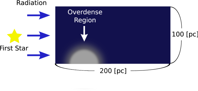
Figure 1: Schematic view of the computational domain. The shadowed region is formed behind the over dense region , while the other region is exposed to radiation field.

2.4 Setup

We consider a mini-halo in the IGM at redshift $z\simeq 20$ exposed to an intense radiation flux from a nearby first star. We assume that the dark matter density profile of the mini-halo is described by the NFW profile (Navarro et al., 1997)

$$\rho_{\rm DM}\left(r\right)=\frac{\rho_{\rm s}}{\left(r/r_{\rm s}\right)\left(1+r/r_{\rm s}\right)^{2}},$$ (12)

where $r$ is the radial destance from the center of halo. $\rho_{\rm s}$ and $r_{\rm s}$ are a characteristic density and radius, which are determined by a halo mass $M_{\rm halo}$ collapsing at redshift $z$ (Prada et al., 2011). We assume the gas density profile is a core-halo structure with $\rho\propto r^{-2}$ envelope. The core radius $r_{\rm c}$ is determined by the core density and the total gas mass $\left(M_{\rm gas}=\left(\Omega_{\rm B}/\Omega_{\rm M}\right)M_{\rm halo}\right)$. We study various cases of core densities $\left(n_{\rm 0}{\rm cm}^{-3}\right)$, the halo mass $M_{\rm halo}$ and distances between the source star and halo center $\left(D{\rm kpc}\right)$. We assume stationarity of the mini-halo with respect to the source star. This assumption is based upon the fact that the the change of distance between the star and the halo due to the relative motion is smaller than $D$, if we consider the cosmic expansion. We remark that in case the neighboring overdense region and the source star is contained in a same halo of $>10^{7}M_{\odot}$, change of the distance due to the velocity dispertion of the halo could have significant effect especially for low mass source stars.

Initially, the ambient gas is assumed to be neutral when the source star is turned on. The initial number density of the ambient gas in the intergalactic space is $n_{\rm IGM}=10^{-2}{\rm cm}^{-3}$. We assume that the initial temperature is $500{\rm K}$. We perform two-dimensional simulations in the cylindrical coordinates assuming axial symmetry. As shown in Figure 1, the computational domain is 100 pc $\times$ 200 pc in $R-z$ plane. We consider source stars of various masses, $M_{\ast}=500$,$300$,$120$,$60$, $25$ and $9M_{\odot}$. The luminosities, effective temperatures and the ages of these stars are taken from the table of Schaerer (2002). The incident radiation from the source star is assumed to be perpendicular to the left edge of the computational domain.

We employ four models (A-D) of different $M_{\rm halo},$$n_{0}$ and $D$ listed in Table 1, these are plausible values of the minihalos in standard $\Lambda$CDM cosmology(see section 3.2). The number of grids we use in these simulations is basically $250\times 500$ which is confirmed to be enough to obtain physical results by the convergence study (see section 3.4).

3 Results

3.1 Typical results

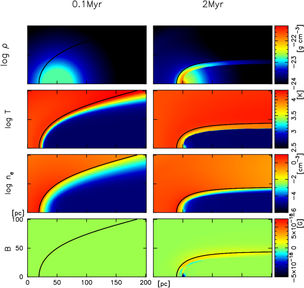
Figure 2: Two snapshots (left:0.1Myr, right:2Myr) for the model A are shown. Four rows correspond to the mass density of gas [${\rm gcm^{-3}}$](top), the gas temperature $[\rm K]$, the number density of electron [${\rm cm^{-3}}$], and the magnetic field strength [$G$], respectively. Black solid lines represent the position of the ionization fronts.

First, we consider a first star of 500 $M_{\odot}$($t_{\rm age}=2\times 10^{6}{\rm yr}$). Figure 2 shows the results for the model A. Two columns correspond to the snapshots at $0.1$Myr and $2$Myr. The top row shows the color contour of the mass density of the gas. The gas density distribution is isotropic at $0.1$Myr, while it is highly disturbed by the radiation flux from the left at $2$Myr. We also can find a shock front at $2$Myr inside the core of the overdense region.

The second and third rows show the maps of the temperature and the electron density. Clearly, an ionization front is generated by the flux from the left, and it propagates into the core of the cloud. It is also worth noting that the pattern of temperature and electron density distribution are similar, but not identical with each other. Slight difference between the two contour maps directly leads to the nontrivial Biermann battery term.

The bottom row shows the distribution of the generated magnetic field strength. As expected, we obtain strong magnetic fields in the neighborhood of the ionization front. In addition, strong magnetic fields is produced at the center of core where the density is the highest. The peak field strength is as strong as $6\times 10^{-18}$G in this case.

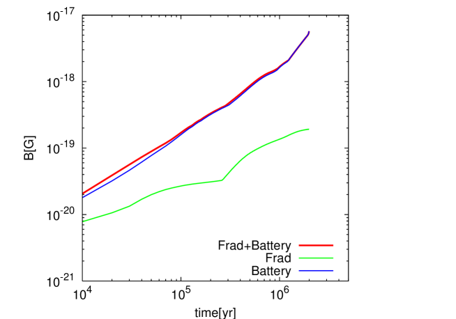
Figure 3: Time evolution of the peak magnetic field for the model A (red). Other two curves correspond to the field generated by Biermann battery (blue) and radiation pressure (green).

In Figure 3, we show the time evolution of the peak magnetic field strength in the simulated region (red curve). We also plot the peak magnetic field generated by the Biermann battery term (blue) as well as the one by the radiation processes (green). The field strength grows almost linearly in this model, and the final strength is as large as $\sim 6\times 10^{-18}$G. We also find that the radiation process is less important than the Biermann battery effect. However, it is still noteworthy that the difference between the two contributions is only a factor of $\sim 10$, although the nature of these processes are very different from each other.

3.2 Dependence on $n_{0}$, $D$, $M_{\ast}$

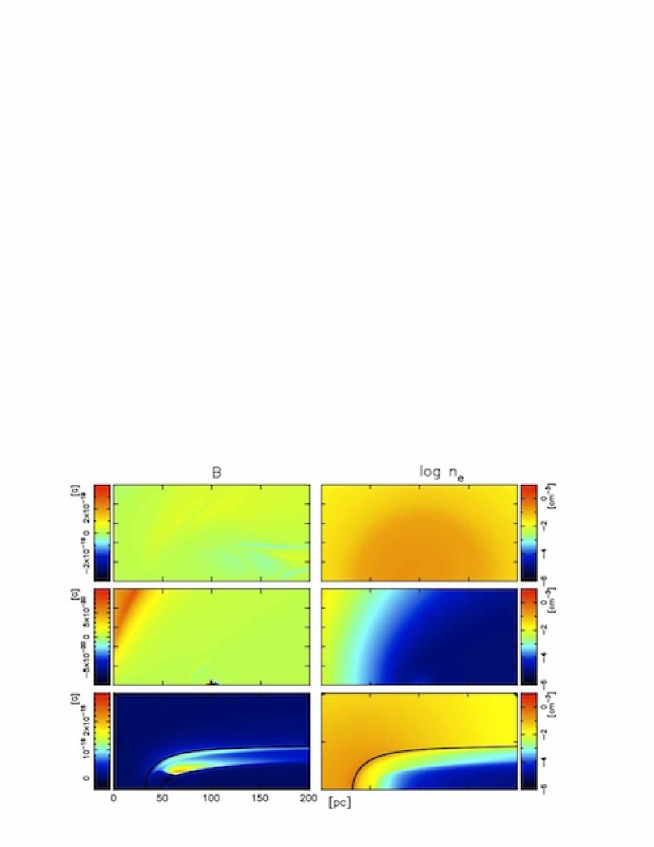
Figure 4: Snapshots at 2Myr for the models B,C and D are shown. Left column : magnetic filed strength, $B$[G] . Right column: electron density, $n_{\rm e}$[cm^-3].

We also investigate the other models of $n_{0}$ and $D$ listed in Table 1. The snapshots at 2Myr of these models (B,C and D from top to bottom) are shown in Figure 4. The left column shows the magnetic field strength, whereas the right column illustrates the number density of electrons. In the model B, the generated magnetic field is of the order of $\sim 10^{-19}$G (top left panel), which is smaller than that in the model A. Since the ionization front is not trapped by the dense core in the model B (top right), the source terms of equation (1) become very small as soon as the ionization front passes through the core. As a result, the magnetic field does not have enough time to grow. In the models C and D, the core is 10 times more distant from the source star than the models A and B. Therefore, the ionization front is trapped at lower density regions, and becomes less sharp than that in model A. Consequently, the generated magnetic field is smaller than that in the model A (middle and bottom row).

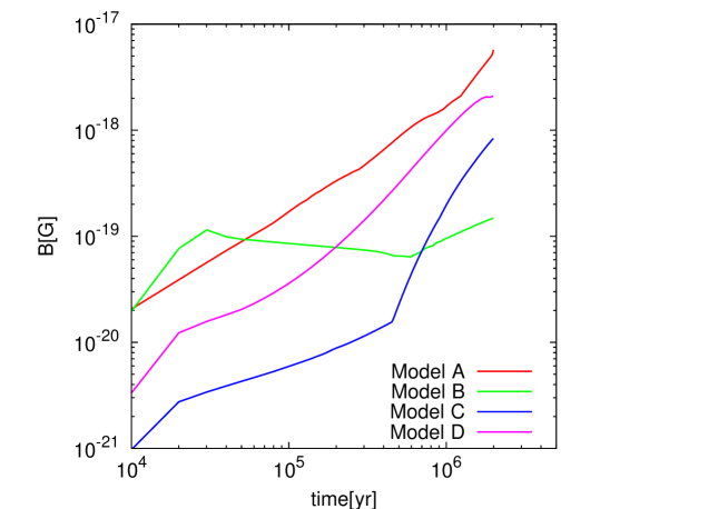
Figure 5: Time evolution of the peak magnetic field for the models A-D.

We also plot the time evolution of the peak field strengths of the models A-D in Figure 5. The models A, C and D mostly increase monotonically, whereas the model B has a clear plateau/decline. Such different behavior also comes from the fact that the ionization front immediately passes through the core in the model B. In such case, the time for the magnetic field to grow is not enough as stated above. In addition, the fluids that host the generated magnetic fields expand due to the thermal pressure of photoionized gas. Such expansion results in the slight decline of the magnetic field strength.

The dependence on the source stellar mass $M_{\ast}$ is also studied. We employ six models of $M_{\ast}=500$,$300$,$120$,$60$,$25$ and $9M_{\odot}$, while the other parameters are same as the model A. Figure 6 shows the peak magnetic field strength as a function of $M_{\ast}$. The peak field strength of each run is evaluated when it gets to the time for the death of the source star. The peak field strength basically increases as the stellar mass becomes more massive. However, the difference between the field strength of $M_{\ast}=9M_{\odot}$ and $500M_{\odot}$ is a factor of 9, which is a small difference for such a mass difference. The reason of this behavior comes from the fact that the more massive the stars are, the more ionizing photons they emit, but also the shorter lifetime they have. These two competing effects cancel with each other.

In any case, the generated magnetic field strengths stay around $10^{-18}-10^{-17}$G, if we consider the stellar mass of $9M_{\odot}$ - $500M_{\odot}$, which range is wide enough for first stars.

The parameters $n_{0}$ and $D$ we employ in this paper are reasonable values. The baryonic density of the virialized halo at $z=20$ is $\sim 1{\rm cm}^{-3}$ , and the sizes of the first halos are $\lesssim 100$pc. In addition, the radii of cosmological HII regions in the numerical simulations are a few kpc (e.g., Yoshida et al., 2007). Thus, our models A-D are reasonable for the standard cosmological model.

To summarize the results of this section (3.2), the magnetic field strength generated around a first star is $10^{-19}{\rm G}<B<10^{-17}$G for $M_{\ast}=500M_{\odot}$, and a factor of a few smaller for less massive stars.

3.3 Coherence length

In addition, we also remark that the coherence length of the magnetic field. Due to the limited computational resource, we employ rather small box size ($\sim 200$pc). The resultant coherence length of the magnetic field clearly exceeds the box size in most of the cases. In addition, if the ionization structure is more or less similar to that of our previous results in ADS10, the coherence length will be as large as $\sim 1$kpc, which is the size of the shadow.

3.4 Convergence check

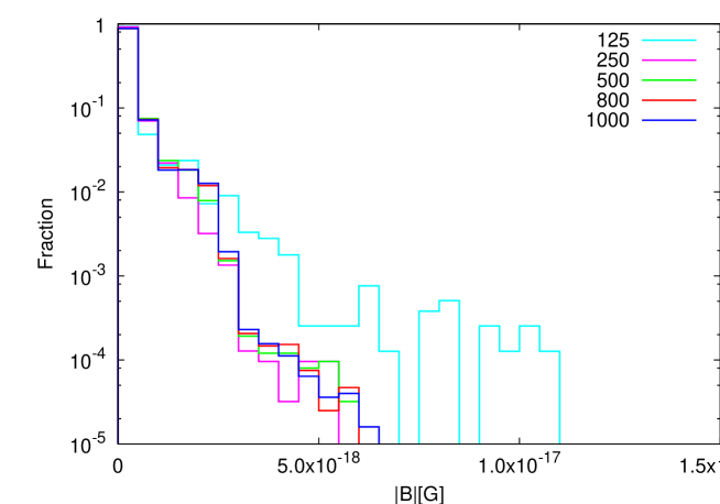
Figure 7: Magnetic field probability distribution functions are plotted for various $N_{Z}$.

Since the equation of the magnetic field generation (1) includes spatial derivatives in its source terms, we have to pay attention to the effects of the cell size on our numerical results. We check the numerical convergence of the magnetic field strengths for the model A. We perform runs with $N_{R}\times N_{z}=63\times 125,125\times 250,250\times 500({\rm canonical}),400\times 800,500\times 1000$, where $N_{R}$,$N_{Z}$ is the number of grids in $R$-axis and $z$-axis, respectively. In Figure 7, the magnetic field probability distribution functions (PDFs) of these runs are plotted. The axis of abscissas is the absolute value of the magnetic field strength, while the vertical axis represents the fraction of grid cells that fall in the range of $[B,B+\Delta B]$, where $\Delta B=5\times 10^{-19}$G. The peak field strength decline as the number of grids increases. However, the peak field strength converges $\sim 6\times 10^{-18}$G and PDFs show similar distributions for $N_{R}\times N_{Z}\geq 250\times 500$. Therefore, the numerical results of the simulations converge very well at $N_{R}\times N_{Z}=250\times 500$, which we use in other runs.

4 Discussions

In this paper, we investigate the magnetic field generated by first stars. As a result, the maximal magnetic field strength is $\lesssim 10^{-17}$G, mainly generated by the Biermann battery mechanism.

In fact, the order of magnitude of the magnetic field generated by the Biermann battery could be assessed as

$$B\sim\frac{c}{n_{e}^{2}e}\left(\frac{n_{e}}{\Delta r}\right)\left(\frac{p_{e}}{\Delta r}\right)\sin\theta\;t_{\rm age}$$

$$\sim 5.0\times 10^{-17}{\rm G}\left(\frac{t_{\rm age}}{2{\rm Myr}}\right)\left(\frac{\sin\theta}{0.1}\right)\left(\frac{\Delta r}{1{\rm pc}}\right)^{-2}\left(\frac{T}{10^{4}{\rm K}}\right),$$ (13)

where $\Delta r$ denotes the typical length of $n_{\rm e}$ and $p_{\rm e}$ change significantly, $\theta$ is the angle between $\bm{\nabla}n_{\rm e}$ and $\bm{\nabla}T$. The resultant value of above equation is roughly consistent with the results of our numerical simulations.

We find the relative importance of the Biermann battery effect versus the radiative processes in this paper. However, this is only relevant for present setup, because the two effects depend differently on various parameters. In particular, the Biermann battery effect do not depend on the flux of the source star directly (see eq.13), whereas the radiation force is proportional to the flux. This means if consider the magnetic field generation process in the very neighbor of the source objects, such as the accretion disks of the protostars/black holes, radiative processes could play central roles in the generation of magnetic field. We will study this issue in the near future.

The field strength obtained in this paper is similar to the results of Xu et al. (2008), in which they investigated magnetic fields in collapsing mini-halos/prestellar cores. If we assume that the magnetic field generated around first stars are brought into another prestellar core, and evolve during the collapse of the primordial gas in a similar way to Xu et al. (2008), the magnetic field will be amplified up to $\sim 10^{-13}$ G at $10^{3}{\rm cm}^{-3}$. However, this magnetic field will not affect subsequent star formation, since the magnetic field strength required for jet formation(Machida et al., 2006) and MRI activation(Tan & Blackman, 2004) is $10^{-10}-10^{-9}$G at $10^{3}{\rm cm}^{-3}$, if we assume simple flux freezing condition. On the other hand, recent studies suggest that weak seed magnetic field is amplified by the turbulence during the first star formation(Schleicher et al., 2010; Sur et al., 2010). In Sur et al. (2010), weak seed magnetic fields are exponentially amplified by small-scale dynamo action if they employ sufficient numerical resolutions. In this case, the magnetic fields generated by the first stars in this paper might be amplified and affect subsequent star formation. However, these studies assume a priori given turbulence and initial magnetic field. To try to settle this issue, we need cosmological MHD simulations with very high resolution.

5 Summary

In summary, we have investigated the magnetic field generation process by the radiative feedback of first stars, including the effects of radiation force and the Biermann battery. As a result, we found $10^{-19}{\rm G}\lesssim B\lesssim 10^{-17}$G on the boundary of the shadowed region, if we take reasonable parameters expected from standard theory of cosmological structure formation. The resultant field strength with a simple assumption of flux freezing suggests that the such magnetic field is unimportant for the star formation process. However, it could be important if the magnetic field is amplified by turbulent motions of the star forming gas could.

We appreciate the anonymous referee for helpful comments. We also thank N.Tominaga and M.Ando for fruitful discussions. This work was supported by Ministry of Education, Science, Sports and Culture, Grant-in-Aid for Scientific Research (C), 22540295.

Model	A	B	C	D
$M_{\rm halo}[h^{-1}M_{\odot}]$	$5\times 10^{6}$	$1\times 10^{5}$	$5\times 10^{6}$	$1\times 10^{5}$
$n_{0}[{\rm cm^{-3}}]$	10	1	10	1
$D[{\rm kpc}]$	0.2	0.2	2	2
Magnetic field [G]	$5.7\times 10^{-18}$	$1.5\times 10^{-19}$	$8.4\times 10^{-19}$	$2.1\times 10^{-18}$

Table 1: The peak magnetic field strengths of four models of $M_{\ast}=500M_{\odot}$.

Figure 6: The maximal magnetic field strength for $D=200$pc, $n_{0}=10{\rm cm^{-3}}$, with various $M_{\ast}$.

References

- Abel, Bryan, Norman (2002) Abel, T., Bryan, G. L., & Norman, M. L. 2002, Science, 295, 93
- Ando et al. (2010) Ando, M., Doi, K., & Susa, H. 2010, ApJ, 716, 1566
- Barrow et al. (1997) Barrow, J. D., Ferreira, P. G., & Silk, J. 1997, Physical Review Letters, 78, 3610
- Biermann (1950) Biermann, L. 1950, Zs. Naturforsch., 5a, 65
- Blasi et al. (1999) Blasi, P., Burles, S., & Olinto, A. V. 1999, ApJ, 514, L79
- Bromm, Coppi & Larson (2002) Bromm, V., Coppi, P. S., & Larson, R. B. 2002, ApJ, 564, 23
- Clark et al. (2011a) Clark, P. C., Glover, S. C. O., Smith, R. J., Greif, T. H., Klessen, R. S., & Bromm, V. 2011, Science, 331, 1040
- Clark et al. (2011b) Clark, P. C., Glover, S. C. O., Klessen, R. S., & Bromm, V. 2011, ApJ, 727, 110
- Fukugita & Kawasaki (1994) Fukugita, M., & Kawasaki, M. 1994, MNRAS, 269, 563
- Gnedin et al. (2000) Gnedin, N. Y., Ferrara, A., & Zweibel, E. G. 2000, ApJ, 539, 505
- Greif et al. (2011) Greif, T., Springel, V., White, S., Glover, S., Clark, P., Smith, R., Klessen, R., & Bromm, V. 2011, arXiv:1101.5491
- Ichiki et al. (2006) Ichiki, K., Takahashi, K., Ohno, H., Hanayama, H., Sugiyama, N. 2006, Sci, 311, 8271
- Kitayama et al. (2004) Kitayama, T., Yoshida, N., Susa, H., & Umemura, M. 2004, ApJ, 613, 631-645
- Kulsrud et al. (1997) Kulsrud, R. M., Cen, R., Ostriker, J. P., & Ryu, D. 1997, ApJ, 480, 481
- Langer et al. (2003) Langer, M., Puget, J., Aghanim, N. 2003, Phys. Rev D, 67, 43505
- Machida et al. (2006) Machida, M.N., Omukai, K., Matsumoto, T., Inutsuka, S. 2006, ApJ, 647, L1
- Machida et al. (2008) Machida, M. N., Matsumoto, T., & Inutsuka, S.-i. 2008, ApJ, 685, 690
- Maki & Susa (2004) Maki, H., Susa, H. 2004, ApJ, 609, 467
- Maki & Susa (2007) Maki, H., Susa, H. 2007, PASJ, 59, 787
- Nakamura & Umemura (2001) Nakamura, F., & Umemura, M. 2001, ApJ, 548, 19
- Nakano & Umebayashi (1986a) Nakano, T., & Umebayashi, T. 1986, MNRAS, 221, 319
- Nakano & Umebayashi (1986b) Nakano, T., & Umebayashi, T. 1986, MNRAS, 218, 663
- Navarro et al. (1997) Navarro, J. F., Frenk, C. S., & White, S. D. M. 1997, ApJ, 490, 493
- Omukai (2000) Omukai, K. 2000, ApJ, 534, 809
- Omukai & Yoshii (2003) Omukai, K., & Yoshii, Y. 2003, ApJ, 599, 746
- Prada et al. (2011) Prada, F., Klypin, A. A., Cuesta, A. J., Betancort-Rijo, J. E., & Primack, J. 2011, arXiv:1104.5130
- Schaerer (2002) Schaerer, D. 2002, A&A , 382, 28
- Schleicher et al. (2009) Schleicher, D. R. G., Galli, D., Glover, S. C. O., Banerjee, R., Palla, F., Schneider, R., & Klessen, R. S. 2009, ApJ, 703, 1096
- Schleicher et al. (2010) Schleicher, D. R. G., Banerjee, R., Sur, S., Arshakian, T. G., Klessen, R. S., Beck, R., & Spaans, M. 2010, arXiv:1003.1135
- Sethi et al. (2008) Sethi, S. K., Nath, B. B., & Subramanian, K. 2008, MNRAS, 387, 1589
- Sethi et al. (2010) Sethi, S., Haiman, Z., & Pandey, K. 2010, ApJ, 721, 615
- Seshadri & Subramanian (2009) Seshadri, T. R., & Subramanian, K. 2009, Physical Review Letters, 103, 081303
- Smith et al. (2011) Smith, R. J., Glover, S. C. O., Clark, P. C., Greif, T., & Klessen, R. S. 2011, arXiv:1103.1231
- Stacy et al. (2010) Stacy, A., Greif, T. H., & Bromm, V. 2010, MNRAS, 403, 45
- Sur et al. (2010) Sur, S., Schleicher, D. R. G., Banerjee, R., Federrath, C., & Klessen, R. S. 2010, ApJ, 721, L134
- Tan & Blackman (2004) Tan, J. C., & Blackman, E. G. 2004, ApJ, 603, 401
- Turner& Widrow (1988) Turner, M.S., Widrow, L.M. 1988, Phys. Rev.D , 37, 2743
- Vallée (2004) Vallée, J. P. 2004, New A Rev., 48, 763
- Xu et al. (2008) Xu, H., O’Shea, B., Collins, D., Norman, M., Li, H., & Li, S. 2008, ApJ. 688, L57
- Yabe & Aoki (1991) Yabe, T., Aoki, T., 1991, Comput.Phys.Commun, 66, 219
- Yoshida (2006) Yoshida, N. 2006, New Astronomy Review, 50, 19
- Yoshida et al. (2007) Yoshida, N., Oh, S. P., Kitayama, T., & Hernquist, L. 2007, ApJ, 663, 687